1. Electronic copy available at: http://ssrn.com/abstract=2554642
1
Portfolio Construction and Tail Risk
Chris Downing, Ananth Madhavan, Ajit Singh and Alex Ulitsky*
January 2015
Abstract
In the wake of the financial crisis, investors are increasingly concerned with ways to
mitigate extreme losses. We analyze various approaches to enhancing traditional
portfolio construction with tail-risk control. Interestingly, we find investors have better
managed tail-risk using a minimum-volatility overlay strategy than explicitly penalizing
extreme losses via conditional value-at-risk (CVaR). From a practical perspective, this
solution can be cheap and easy to implement because it will not result in a rebalancing
of the fund, and various minimum-volatility products are readily available on the
market.
* Chris Downing, Ananth Madhavan, and Alex Ulitsky are at BlackRock, Inc. Ajit Singh is Chief Risk Officer of the
United Nations UNJSPF/Investments. Of course, any errors are entirely our own. The views expressed here are
those of the authors alone and not necessarily those of BlackRock, its officers, or directors or of the United
Nations. This note is intended to stimulate further research and is not a recommendation to trade particular
securities or of any investment strategy.
© 2015 BlackRock, Inc. All rights reserved.

2. Electronic copy available at: http://ssrn.com/abstract=2554642
2
1. Introduction
The Financial Crisis of 2008-2009 resulted in extreme losses for many investors, leading to increased
interest in approaches to mitigate so-called “left tail” risk. This paper discusses approaches to
enhancing traditional mean-variance portfolio construction with tail-risk control, a factor important for
investors concerned with extreme losses.
It is well-known (see, e.g., Markowitz (1952)) that when asset returns are jointly normally distributed,
then variance is an appropriate risk measure. Moreover, given a set of expected returns, optimizing a
portfolio under the assumption of normality is straightforward, since the first two moments of returns
completely characterize the distribution of returns. Simplicity and elegance explains the popularity of
mean-variance optimization. Further, minimum-variance portfolios have demonstrated attractive
properties, and a wide set of such products are now available to investors.1
More recently, a growing number of financial practitioners and academics have begun to explore
alternatives to variance as a measure of risk, and approaches to portfolio construction that go beyond
mean-variance optimization.2
On strictly empirical grounds, the empirical distributions of returns of
many financial assets do not appear to be consistent with the assumption of normality—exhibiting left-
skew and/or fat tails— as exemplified in the Financial Crisis. In this situation, the mean-variance
solution is not necessarily optimal. Second, on behavioral grounds, there is a large body of evidence
suggesting that investors fear losses more than they value gains—that is, investors are “loss averse.”
The mean-variance approach is symmetric in its treatment of risk—the variance penalty applies to up-
side risk as much as down-side risk. Post-crisis, regulatory initiatives to guard against systemic risk to
the financial system have further motivated interest in tail risk. Banks are required to monitor and
manage their capital levels against their potential exposures to large losses.
This paper analyzes the benefits and costs of adding a tail-risk penalty to the standard mean-variance
optimization framework using a universe of broadly representative equity and fixed-income exchange-
traded funds (ETFs) as proxies for investible indices. We first look at portfolio constructions employing a
penalty for conditional value-at-risk (CVaR) which captures the left-tail probability mass of the return
distribution. We compare the optimal portfolios obtained in both the minimum-risk context, where
expected returns are zero, and in the alpha context where we use forecasts of excess returns, in order to
build intuition for how penalizing tail-risk affects the constructions.
1
For example, various global and regional minimum-volatility portfolios are available in ETF form. Minimum-variance portfolios
are obtained by carrying out mean-variance optimization with the mean returns all set to zero.
2
See e.g. “Minimizing Shortfall” by L. Goldberg, M. Hayes and O. Mahmoud, January 2011. MSCI Barra Research Paper No. 2011-04,
“Mean-Variance Versus Mean-Conditional Value-at-Risk Optimization” by J. Xiong and T. Idzorek, February 2010. Ibbotson Research Paper.

3. 3
By definition, a focus on tail risk means focusing on relatively rare events, putting a premium on the
number of time periods over which asset returns and other data points can be measured. We address
this issue by building a Monte Carlo simulator that matches the first four moments of the observed
returns, and that mimicks the correlation structure and tail risk properties of the observed data. Using
the simulator, we investigate the finite-sample distribution of the CVaR estimator, both at the individual
instrument level, and at the portfolio level where we study portfolio performance in the out-of-sample
back-test setting.
This analysis produces two main results. First, it’s well-known that data limitations are the main issue in
forecasting tail-risks. A key result of this paper is that, for simulated data samples of less than about 30
years in length, in the zero expected-return case it is not possible on the basis of ex-post CVaR statistics
to differentiate portfolios constructed under minimum-variance from those constructed using
minimum-CVaR. A practical implication of this result is that if tail-risk reduction is an investment goal,
employing a minimum-volatility portfolio exposure is potentially a better way of achieving this goal.
Second, we examine the implications of the tail-risk penalty for portfolio constructions in the alpha
context where we impose expectations for excess returns based on historical returns. Starting from a
mean-variance optimized portfolio, we add the CVaR penalty with increasing weight to see how the
portfolios evolve away from the mean-variance solution as a function of the weight on CVaR. We find
that the CVaR penalty is an effective way to cut tail-risk, both in expected terms and ex-post, provided
one has a significant amount of data with which to measure CVaR. However, the Monte Carlo evidence
indicates that the sampling error of the out-of-sample portfolio CVaR estimator is high (even with a long
series of historical returns), implying that an investor needs to have a high degree of tail-risk aversion
before it would make sense to contemplate the use of a tail-risk penalty. In order to create portfolios
that are sufficiently differentiated in terms of ex-ante tail-risk that one can confidently expect to realize
a difference ex-post, one has to cut expected return significantly via a high weight on the CVaR penalty.
For investors with only modest aversion to tail-risk, the cost in terms of reduced expected return will
probably be too steep.
We next turn to an analysis of the use of the tail-risk penalty for portfolios optimized at the security
level over the MSCI ACWI and S&P500 index constituents. The motivation for this analysis is to explore
the robustness of the Monte Carlo results obtained above. Do the results change when we have
arguably more breadth and confront the optimization with the idiosyncratic risk of equities? Somewhat
surprisingly, we again find that on an ex-post CVaR basis, the minimum-volatility portfolio is superior to
the minimum-CVaR portfolio. Digging a bit deeper, one of the key features of the minimum-volatility
portfolio is, as the name suggests, a significant underweight of the portfolio exposure to market
volatility. Interestingly, the volatility style factor exhibits the worst ex-post CVaR reading of all of the
style factors commonly employed in equity factor risk models, for example Barra. This fact does not
seem to be widely recognized, and could be an alternative explanation for the so-called minimum-
volatility anomaly. The anomaly arises because minimum-volatility under-weights volatility exposure
and volatility exposure forecasts tail risk.

4. 4
To follow up on these findings we use historical back-tests at the security level to test the benefits in
terms of ex-post CVaR from adding total- or tail-risk penalties to the conventional mean-variance
portfolio construction. Consistent with our prior results, for long-only equity portfolio constructions the
tail-risk penalty yieded better CVaR values on ex-ante basis, but fails to provide any benefit on an ex-
post CVaR basis.3
Together these results suggest that CVaR minimization approaches based on historical returns do not
produce portfolios with robust ex-post tail-risk properties. Conventional factor risk models appear to
enjoy an advantage in forecasting tail-risk, likely by incorporating significantly more asset-level
information than just returns, and by updating this information often relative to the extreme events that
drive tail-risk computations like CVaR. Below we provide some empirical results that are supportive of
this explanation.
The results suggest that, in practice, investors can reduce extreme loss exposure by adding a total risk
penalty to the standard mean-variance portfolio construction process, and we highlight a cost-benefit
approach that can be used to identify an optimal weight on the total risk penalty term. As an
illustration, we use the S&P500 constituent data to analyze the effects of the tail-risk penalty in the
alpha context, here in terms of the Volatility and Momentum factor portfolios. As noted above, the
Volatility portfolio has the worst tail-risk properties among the style factors, and Momentum is a close
second. The question we ask was if by adding a CVaR penalty we can produce Volatility and/or
Momentum portfolios with less tail risk? Our results are not definitive owing to our use of monthly
returns, but we find encouraging evidence that this might be possible. In other words, the tail-risk
penalty “re-mixes” the exposures so that we achieve the same expected alpha, but by putting weight on
exposures that, on a portfolio level, deliver lower realized tail-risk. The differences in ex-post CVaR are
not very large, however, and probably not statistically significant. We suspect that one would need to
use a longer series of weekly or daily data in order to achieve more definitive results. There is the
possibility, however, that the factors are correlated to tail-risk in a way that precludes a re-mixing.
As an alternative to the total-risk penalty approach, one can simply use a minimum-volatility strategy as
a portfolio overlay. This solution is cheap and easy to implement because it will not result in a
rebalancing of the fund, and various minimum-volatility products are readily available on the market. In
the last section of the paper we provide some guidance on the effectiveness of this approach.
The remainder of the paper is organized as follows. In Section 2, we review the definition and
properties of CVaR as a risk metric and discuss the data that we use in the ETF analysis. Section 3
presents our ETF-based analysis and Monte Carlo results. Section 4 presents the security-level analysis,
and Section 5 concludes with some thoughts for future work.
3
Note that adding a total risk penalty is equivalent to blending in a minimum-volatility exposure, because a total
risk optimization with zero expected returns produces the minimum-volaility portfolio.

5. 5
2. Measuring Tail Risk
As mentioned at the outset, ex-post asset returns appear to be non-normal; some evidence along these
lines is shown in Panel A of Table 1. The table shows the first four moments of monthly excess returns
on some of the assets we use in our study. Here we employ ETFs to provide exposure to relatively
illiquid sectors like corporate credit (CRED) and emerging market equity (EEM), along with standard
exposures in government bonds (GOVT) and large-cap equities (IVV). The excess returns are computed
over the 1-month Treasury Bill return. The time period is January 2004 – December 2013, over which
time we’re able to construct consistent monthly NAV-based total return series for the ETFs or their
underlying indexes4
.
As can be seen, none of these assets exhibit returns that appear strictly consistent with normality.
Equities and corporate credit exhibit left skew, while government bonds exhibit right-skew. And all of
the returns appear to be drawn from fat-tailed distributions (kurtosis > 3). Figure 1 displays the time-
series of excess returns for the instruments, where it’s apparent that periods of extreme drawdowns
tend to cluster around specific events, and periods of high volatility and heightened downside risk tend
to be persistent. Figure 2 shows the cumulative excess returns for a slightly different perspective where
its clear that periods of heightened volatility tend to correspond to drawdowns in performance.
The correlation structure is shown in Panel B. The GOVT fund returns are positively correlated with
credit, CRED, and negatively correlated with both equity fund returns. Credit is positively correlated to
equity, and the two equity funds are highly correlated with one another.
Table 1: Summary Statistics for Observed Excess Returns
Panel A: Univariate Statistics
4
Time period is January 2004 – December 2013. ETF NAV-based total returns are used where available, and funds’ underlying
index returns are used for the period prior to the ETFs’ inception. For GOVT: Barclays U.S. Treasury Bond Index returns are used
prior to the fund’s inception. For CRED: Barclays U.S. Credit Bond Index returns are used prior to inception. For IVV and EEM:
ETF returns are used for the entire period.
AUM Standard
Ticker Fund Name ($mil) Mean Deviation Skew Kurtosis CVaR (.05) CVaR (.01)
GOVT ISHARES CORE US TREASURY BOND ETF 240 0.0257 0.0436 0.23 4.7 -0.0226 -0.0307
CRED ISHARES CORE US CREDIT BOND ETF 742 0.0337 0.0570 -0.62 8.1 -0.0355 -0.0627
IVV ISHARES CORE S&P 500 ETF 68,722 0.0552 0.1458 -0.86 5.1 -0.0975 -0.1369
EEM ISHARES MSCI EMERGING MARKETS ETF 36,157 0.0840 0.2362 -0.53 4.2 -0.1422 -0.2064
Note: Mean and Standard Deviation are annualized

6. 6
Panel B: Correlations
Figure 1: Observed Monthly Excess Returns
Figure 2: Observed Cumulative Excess Returns
GOVT CRED IVV EEM
GOVT 1.00 0.53 -0.29 -0.20
CRED 0.53 1.00 0.31 0.41
IVV -0.29 0.31 1.00 0.80
EEM -0.20 0.41 0.80 1.00

7. 7
In light of these results and the various reasons for highlighting downside risk discussed at the outset,
numerous measures of tail risk have been proposed. One such measure is the so-called value-at-risk
(VaR, or “expected shortfall”), which identifies a threshold value of loss beyond which losses occur with
some probability. The VaR concept is widely used; it is the required risk measure for regulatory
reporting by banks under the Basel agreements, for example. But as a risk concept, this metric has a
number of shortcomings, not the least of which is that for especially fat-tailed return distributions the
VaR threshold value might appear to be low, but the actual amount of value-at-risk is high because VaR
does not measure the mass of distribution beyond the threshold value. Owing in part to some of its
problematic statistical properties, it’s relatively difficult to optimize for minimum VaR.
Conditional Value at Risk (CVaR) addresses most of these issues by measuring the average return,
conditional on being less than the VaR threshold:
𝐶𝑉𝑎𝑅 =
1
𝑁
∑ (𝑅 𝑛|𝑅 𝑛 < 𝑉𝑎𝑅),𝑁
𝑛=1 (1)
where N is the number of observations falling into the set of returns satisfying the VaR criterion, 𝑅 𝑛
denotes the nth
return in this set, and 𝑉𝑎𝑅 (< 0) is the Value at Risk criterion. The setting of VaR
defines the fraction of the left tail that goes into the CVaR calculation. We’ll typically focus on settings
delivering 5% or 1% CVaR readings, denoted by CVaR(5%) and CVaR(1%) in what follows.
In the last two columns of Panel A of Table 1 we show the 5% and 1% CVaR values for each asset. The
interpretation of these values is intuitive. Focusing on the S&P 500, for example, conditional on a
monthly return in the lower 5% tail, the expected monthly excess return is -9.75%. The CVaR measure
is also attractive because it’s a coherent risk measure—it exhibits monotonicity, sub-additivity, and
translation invariance.5
A CVaR-optimized portfolio will by construction be VaR-optimal and mean-
variance optimal for normally distributed data.6
This last fact is useful because many times our null
hypothesis is that the data are normally distributed. Given that CVaR is attractive in so many respects,
in what follows we will focus on this measure of tail risk.
3. Portfolio Construction with Tail Risk Control
Earlier we discussed some of the advantages of mean-variance optimization, including its ease of
implementation and familiarity given its role as the workhorse optimization technique in portfolio
construction. In order to retain these advantages while incorporating consideration of tail-risk, here we
examine an objective-function blending both:
𝑚𝑎𝑥ℎ 𝑈(ℎ) = 𝛼(ℎ − ℎ 𝑏) − 𝜆 𝑀𝑉[(ℎ − ℎ 𝑏)𝑉(ℎ − ℎ 𝑏)′] − 𝜆 𝐶𝑉𝑎𝑅 𝐶𝑉𝑎𝑅(ℎ) (2)
5
Rockafellar, R. T. and S. Uryasev. 2002. “Conditional value-at-risk for general loss distributions,” Journal of Banking & Finance.
26:1443-1471.
6
Note that CVaR is proportional to standard deviation for normally distributed data.

8. 8
Under this objective function, the parameter 𝜆 𝐶𝑉𝑎𝑅 ≥ 0 governs the degree to which the CVaR tail-risk
penalty in the second term is incorporated.7
When 𝜆 𝐶𝑉𝑎𝑅 = 0, we perform standard mean-variance
optimization; when 𝜆 𝐶𝑉𝑎𝑅 = 1 we ignore everything other than the left tail and optimize only on CVaR.8
Assuming that one already has a risk-model that can be used to forecast risk for the mean-variance
piece of the optimization, the immediate issue that asserts itself is how to forecast CVaR? The simplest
approach is to calculate CVaR based on historical returns, as we did in Table 1 above, and assume that
this forecasts future CVaR. However, as discussed at the outset a focus on CVAR by definition excludes
95% of the data (or even 99% of the data), focusing attention on a very limited number of observations.
In event terms, the focus is likely to be even more concentrated—extreme left tail draws will cluster in
major events. Thus a 5% CVaR criterion will, except in the longest of time-series, involve a small handful
of major market events. Taken together, these facts imply that any forecast of CVaR based on historical
returns is likely to be inaccurate. One of our goals here is to shed light on the finite-sample accuracy of
CVaR forecasts based on historical returns.
As a starting point in building some understanding of how a CVaR(5%) penalty affects portfolio
construction, we consider some simple portfolios built on the instruments in Table 1. Here we work
entirely in-sample, using all of the data to form our expected excess return views; we use the Mean
excess returns reported in Table 1. The variance-covariance matrix is computed over the entire history
of data, as well, and we compute the CVaR(5%) values using the full sample.
Table 2 shows the portfolios that result under these optimization setups. For comparison, the first
column of results reports the minimum-CVaR portfolio where the expected returns are all set to zero
(‘MinCVaR’) and 𝜆 𝑀𝑉 = 0. The next column (‘MinVol’) reports the results for the minimum-volatility
portfolio where we again set the expected returns to zero but this time set 𝜆 𝐶𝑉𝑎𝑅 = 0. We then move to
some blended portfolios with increasing weight on the mean-variance criterion as we move across the
table from the column labelled ‘CVaR’ to the column labelled ‘MeanVar’, where we report the standard
mean-variance results. For this portfolio, we set 𝜆 𝑀𝑉 = 1.03 and 𝜆 𝐶𝑉𝑎𝑅 = 0 which delivers a portfolio
with expected risk equal to 12.02%.9
The allocation for this portfolio is about 50% equity and 50% fixed-
income, with the equity highly concentrated in EEM and the fixed-income concentrated in GOVT. Here
we are carrying out a total-risk optimization without a benchmark, and as is typically the case the
optimal portfolio will tend to be concentrated and will “barbell” the risks by holding the risky EEM name
and GOVT as a hedge against this. Moving to the left to ‘Blend2’ and ‘Blend1’, we raise the CVaR penalty
7
Note that one could fix, say, 𝜆 𝑀𝑉 = 1 and treat 𝜆 𝐶𝑉𝑎𝑅 as a relative weight. We’ve found it more intuitive and convenient to
use both risk-penalty weights.
8
The optimizations can be carried out using any of a variety of nonlinear optimizers; we use the fmincon() routine packaged
with Matlab. For details on optimizing CVaR using historical returns, see Rockafellar, R. T. and S. Uryasev. 2000. “Optimization
of conditional value-at-risk,” Journal of Risk. 2:21-41.
9
Expected risk is given by 𝐸[𝑉𝑜𝑙] = √ℎ′𝑉ℎ, where h is the column-vector of portfolio holdings and V is the risk-model.
𝐸[𝑅] = ℎ′𝜇 where 𝜇 is the vector of expected excess returns from Table 1.

9. 9
while holding 𝜆 𝑀𝑉 fixed at 1.03. For Blend2, we set 𝜆 𝐶𝑉𝑎𝑅 = 7.0𝑒 − 3, which delivers an expected
volatility of about 10%, and for Blend1 we set 𝜆 𝐶𝑉𝑎𝑅 = 1.4𝑒 − 2 to deliver 8% expected volatility, and for
CVaR we set 𝜆 𝐶𝑉𝑎𝑅 = 3.9𝑒 − 2 to deliver about 6% expected volatility.10
Table 2: Optimization Results for Observed Data
As one might expect, as we increase the CVaR penalty, we mix in more and more GOVT and less CRED
and EEM. Large-cap equity, IVV, participates at about the same level until we boost the CVaR penalty to
its maximum level, taking E[Vol] to down .0618. Comparing the CVaR(.05) levels for the portfolios,
under MeanVar the 5% CVaR reading is -.0720, while for the CVaR portfolio it is -.0373, indicating that
the CVaR penalty has the desired effect of ratcheting down expected tail-risk. This comes at an
expected return penalty, however, of about 160bps, as shown in the row labelled E[R].
Note that the blended solutions are not simply weighted averages of the holdings under the CVaR and
MeanVar portfolio settings – they are more nuanced. This is a reflection of the fact that we’re
optimizing over both penalty functions simultaneously, so the optimizer makes complex tradeoffs across
the assets in order to find the optimal solution.
What’s also interesting is that the MinVol solution is broadly similar to the MinCVaR solution, differing
by only a handful of percentage points in the CRED/IVV allocation, and in terms of the CRED allocation.
In terms of the risk measures, the two approaches are also quite similar: their CVaR(.05) readings differ
by only about 20bps – almost certainly statistically indistinguishable from one another. This basic result:
that the MinVol solution is about the same or better than the MinCVaR solution—measured across a
range of different criteria—is robust across different asset universes, using 1% or 5% CVaR, and across
different time periods. What is going on? Why does MinVol seem come close to beating MinCVaR at its
own game? The answer to this question has broad implications for how one attempts to deal with tail
risk. And the answer may shed light on the root cause of the “minimum volatility anomaly” laid out in
the introduction—does reduction in tail-risk exposure explain the anomaly?
10
The variance and CVaR penalties are on different scales, and their weights don’t appear to have intuitive interpretations. This
is why we use E[Vol] to calibrate the models. Note that one could also increase the value of 𝜆 𝑀𝑉 to reduce E[Vol], producing a
sequence of portfolios converging onto the MinVol solution shown in the second column, while boosting 𝜆 𝐶𝑉𝑎𝑅 will lead to a
sequence of portfolios converging onto the MinCVaR solution shown in the first column.
Ticker MinCVaR MinVol CVaR Blend1 Blend2 MeanVar
GOVT 91.5% 86.1% 74.9% 61.4% 49.4% 34.6%
CRED 2.4% 0.0% 0.0% 0.0% 4.4% 12.2%
IVV 6.1% 13.9% 0.0% 8.6% 7.4% 5.9%
EEM 0.0% 0.0% 25.1% 30.1% 38.8% 47.3%
E[R] 0.0277 0.0298 0.0403 0.0458 0.0509 0.0560
E[Vol] 0.0391 0.0372 0.0618 0.0800 0.0997 0.1202
CVaR(.05) -0.0198 -0.0218 -0.0373 -0.0490 -0.0604 -0.0720
CVaR(.01) -0.0315 -0.0333 -0.0550 -0.0715 -0.0912 -0.1121

10. 10
Another question concerns the precision with which we’re able to differentiate the CVaR estimates
across the portfolios. Can we distinguish, say, Blend2 vs MinVar on the basis of CVaR?
Simulations
As noted earlier, a historical analysis is limiting in that the returns are given and we have no way to
analyse how different properties of returns might play out in terms of the relative performance of
portfolios built using mean-variance versus portfolios built using CVaR. In order to gain more insight, we
turn to Monte Carlo simulation where we can control the return-generating process.
We first build a Monte Carlo simulator that matches the first four moments of returns for the assets in
our universe, and that produces realistic CVaRs for the assets. A design objective is that the return-
generating process should be grounded in a plausible economic story for how extreme tail draws come
about, and for how asset returns behave in these tail events.
The simulator that we develop is based on ideas proposed by Andrew Lo in the Financial Analysts
Journal.11
In order to generate skew and kurtosis in the simulated returns the model incorporates
features inspired by the notion of “phase-locking” processes in the physical sciences. A phase-locking
process is one where seemingly uncorrelated processes can, under certain conditions, become highly
correlated. In the physical sciences, the chirping of crickets is one example of phase-locking. In finance,
economic shocks that cause panic in markets lead to asset returns exhibiting many of the features of
phase-locking. In such events, investors tend to sell out of risky assets and buy safe-haven assets such
as Treasury bonds or they move into cash. These flows produce asset returns that are more highly
correlated than in “normal” times—positively correlated within equities and within bonds, and
negatively correlated across equity and bonds. In these events, volatility in returns also tends to be
heightened. These features—shifts in correlations & heightened vol—tend to persist. We’ll attempt to
capture these properties in our phase-locking setup.
In “normal” times, we use a simple model calibrated to observed returns to drive the simulations. This
portion of the process produces normally-distributed returns, so in “normal” times there is no difference
between the mean-variance and minimum-CVaR portfolios. The phase-locking process is what produces
the features of returns that potentially drive a wedge between the two approaches.
Using a somewhat simplified version of the model in Lo (2001), returns across the K instruments are
generated by the following model:
𝑅𝑖𝑡
𝑒
= 𝜇𝑖 + 𝐼𝑡 𝑍𝑖𝑡 + 𝜖𝑖𝑡 (3)
where 𝑅𝑖𝑡
𝑒
is the excess return (over 1-mth T-Bills) on asset i = 1, 2, …, K over period t, 𝐼𝑡 𝑍𝑖𝑡 is the “phase-
locking” element, and 𝜖𝑖𝑡 is the “normal times” risk of asset i over time t. We assume that 𝑍𝑖𝑡 and 𝜖𝑖𝑡
11
Lo, A. W. 2001. “Risk management for hedge funds: Introduction and overview,” Financial Analysts Journal. 57(6):16-33.

11. 11
are mutually i.i.d. with 𝐸[𝑍𝑖𝑡] = 𝜈𝑖, 𝑉𝑎𝑟[𝑍𝑖𝑡] = 𝛾𝑖
2
𝜎 𝑍
2
, 𝐸[𝜖𝑖𝑡] = 0, 𝑉𝑎𝑟[𝜖𝑖𝑡] = 𝜎𝑖
2
, and the normal-times
risks are correlated according to 𝐸[𝜖𝑖𝑡 𝜖𝑗𝑡] = 𝜌𝑖𝑗. The indicator variable 𝐼𝑡 = 1 in phase-lock periods, and
zero otherwise. The indicator follows a Markov process defined by transition probabilities 𝑝𝑖𝑗𝑡 =
𝑝𝑟𝑜𝑏(𝐼𝑡 = 𝑖|𝐼𝑡−1 = 𝑗) for i = 0, 1 and j = 0, 1.
We calibrate this process so that our simulated data match the first four moments of the observed data.
This is accomplished using the following recipe:
1. Set 𝑝01𝑡 =
1
12∗20
, 𝑝00𝑡 = 1 − 𝑝01𝑡, 𝑝10 = .15, 𝑝11 = .85. These settings produce a crisis
period (phase-lock) once every 20 years, on average, and the episodes of phase-lock
average eight months in length before we revert back to normal times.
2. Set 𝜎 𝑍 = .1. This is sufficient to put a significant amount of correlated volatility into the
returns in the phase-lock periods.
3. Make N draws from the multivariate normal distribution defined by 𝜇 and Σ, where 𝜇 is
the K x 1 vector of average excess returns over the instruments, and Σ is the K x K
variance-covariance matrix of excess returns. Label these draws 𝑅̃ 𝑖𝑛
𝑒
.
4. Iterating through the n = 1, 2, …, N simulated periods, make a draw of the state for each
period. Draw a uniform [0, 1] variable, 𝑈 𝑛. If last period was a normal state, then if
𝑈 𝑛 ≤ 𝑝01, then the current state is a phase-lock state, otherwise we stay in the normal
state. If the last state was phase-lock, then if 𝑈 𝑛 ≤ 𝑝10, the current state is normal,
otherwise we stay in phase-lock.
5. Make 𝑁(0, 0.12
) draws, 𝑍 𝑛 for n = 1, 2, …, N. If 𝐼 𝑛 = 1, add 𝜈𝑖 + 𝛾𝑖 𝑍 𝑛 to 𝑅̃ 𝑖𝑛
𝑒
for each i.
The parameter 𝜈𝑖 will typically be negative for negatively skewed instruments; the
parameter 𝛾𝑖 scales the shock Z for each instrument so that we can match the kurtosis
of the observed returns. Note that this process cannot mimic platykurtic data because
at root the returns are multivariate normal; we can only increase the fourth moment via
this mechanism.
6. Re-scale the simulated returns by asset so the variance of the simulated data matches
that of the observed returns. The returns will remain fat-tailed.
7. Shift the returns by asset so that the average simulated return matches the average
observed return. The returns will remain skewed.
8. Compute the skew and kurtosis of the simulated data; adjust the 𝜈 and 𝛾 until the skew
and kurtosis of the simulated data match the observed data. Note that these
parameters must be adjusted simultaneously; a simple nonlinear optimizer and a
quadratic loss function in the observed & simulated moments is sufficient to deliver a
match of the moments for most instruments.
Using the simulator calibrated as described, we generate 250,000 simulated draws of returns. Table 3
provides summary statistics on the simulated data. Comparing Table 3 with Table 1, one can see that
the simulator is doing a reasonably good job of matching the first four moments and the correlation
structure of the instruments. Similarly, the CVaRs of the simulated returns are close to those observed

12. 12
on the instruments, as well. While there are surely features of the data that the simulator is missing, it
does seem to sufficiently describe the data that we can use it to understand more about the properties
of CVaR-optimized portfolios and the precision with which we can estimate CVaR in finite samples.
Table 3: Summary Statistics for Simulated Returns (N = 250,000)
Panel A: Univariate Statistics
Panel B: Correlations
Table 4 displays the portfolios that result when we repeat the optimizations done earlier on the
observed returns. Here we use the full set of 250,000 simulated observations, and we keep the same
settings for the penalty-weights 𝜆 𝑀𝑉 and 𝜆 𝐶𝑉𝑎𝑅. As should be expected, at the 5% level the results are
very close to those for the observed data. At the more extreme CVaR(1%) level, the CVaR penalty at a
given weight is greater, resulting in portfolios that converge more quickly onto to the MinCVaR solution
as we move from right to left across the last four columns.
Monte Carlo simulator in-hand, we are now in a position to analyse the finite-sample distribution of the
CVaR estimator, the usual caveat in mind that everything here is conditional on the properties of our
simulator. First, we look at this at the instrument level. For each of the tickers, we divide the simulated
data into non-overlapping sub-periods. In each sub-period, we make a computation of CVaR at the 5%
and 1% levels. Finally, we fit a kernel density estimator to the resulting CVaR values to get a feel for the
distribution of values. We repeat this process for sub-periods of different lengths. The density
estimates are shown in Figures 3 & 4. With anything less than 100 years of data, the sampling error in
the CVaR estimates is high and the distributions exhibit fat tails. For IVV and EMM, we have a
particularly hard time distinguishing the CVaR readings.
Asset
Mean
Standard
Deviation
Skew Kurtosis
CVaR
(0.05)
CVaR
(0.01)
GOVT 0.0257 0.0436 0.27 4.8 -0.02 -0.0329
CRED 0.0337 0.0570 -0.58 7.8 -0.03 -0.0623
IVV 0.0552 0.1458 -0.76 5.1 -0.10 -0.1605
EEM 0.0840 0.2362 -0.51 4.2 -0.16 -0.2370
GOVT CRED IVV EEM
GOVT 1.00 0.57 -0.29 -0.22
CRED 0.57 1.00 0.32 0.40
IVV -0.29 0.32 1.00 0.84
EEM -0.22 0.40 0.84 1.00

13. 13
Table 4: Optimization Results for Simulated Data
The phase-lock process exerts a clear influence on the finite-sample distributions. When the size of the
sample is small compared to the incidence of phase-lock events, a relatively large share of the extreme
observations come from the normal-times distribution, and this is reflected in the CVaR distributions
having a bi-modal character to them. This is most obvious for IVV and EEM with the sample size of 20
years. As the sample-size grows relative to the incidence of phase-lock events, we draw a higher share
of extreme observations from the phase-lock periods, and the CVaR distributions more consistently
reflect the properties of the return distribution in phase-lock. Given that phase-lock events are rare and
short, this process of convergence is slow. It’s only with about 120 or more years of data that the
distributions start to really stabilize and additional observations have little marginal impact on the shape
of the distribution of CVaRs.
Unfortunately, for most instruments we will typically have only 30 years of data on returns, and for
many asset classes this is being generous. In a back-test exercise, we have to use a portion of any
available data to seed the back-test return forecasts, risk model, and CVaR forecasts, further reducing
the sample-size that can be used in the back-test itself. Given these limitations, how precise are the
estimates of portfolio-level ex-post CVaR? Can we actually distinguish portfolios on the basis of ex-post
CVaR performance? The Monte Carlo simulator is useful for shedding light on this question.
Full-Sample 5% CVaR
Asset MinCVaR MinVol CVaR Blend-1 Blend-2 Mean-Var
GOVT 89.3% 86.1% 76.7% 66.9% 52.3% 36.8%
CRED 0.0% 0.0% 0.0% 0.1% 6.6% 12.7%
IVV 10.8% 13.9% 0.0% 0.0% 0.0% 0.0%
EEM 0.0% 0.0% 23.3% 32.9% 41.1% 50.5%
E[R] 0.0289 0.0298 0.0393 0.0449 0.0502 0.0561
E[Vol] 0.0375 0.0371 0.0579 0.0770 0.0969 0.1205
CVaR(.05) -0.0211 -0.0213 -0.0357 -0.0489 -0.0626 -0.0788
CVaR(.01) -0.0334 -0.0351 -0.0587 -0.0779 -0.0980 -0.1214
Full-Sample 1% CVaR
Ticker MinCVaR MinVol CVaR Blend1 Blend2 MeanVar
GOVT 95.1% 86.1% 88.9% 73.5% 62.0% 36.8%
CRED 0.0% 0.0% 0.0% 0.0% 0.0% 12.7%
IVV 4.9% 13.9% 0.0% 0.0% 0.0% 0.0%
EEM 0.0% 0.0% 11.1% 26.5% 38.0% 50.5%
E[R] 0.0272 0.0298 0.0322 0.0412 0.0479 0.0561
E[Vol] 0.0400 0.0371 0.0418 0.0639 0.0880 0.1205
CVaR(.05) -0.0219 -0.0213 -0.0241 -0.0399 -0.0564 -0.0788
CVaR(.01) -0.0322 -0.0351 -0.0389 -0.0649 -0.0885 -0.1214
Note: E[R] and E[Vol] are annualized.

14. 14
Figure 3: Finite-Sample Distributions of CVaR(5%) Estimators
Figure 4: Finite-Sample Distributions of CVaR(1%) Estimators

15. 15
To do this, we again divide our simulated data into non-overlapping sub-periods, here each of 30 years
length. In each sub-period, we start at the 15 year point and use the simulated returns up to that point
to build a variance-covariance matrix to drive the mean-variance portion of a portfolio construction, and
we use the returns to drive a min-CVaR component. To keep things simple in terms of interpretation,
we assume we “know” the expected returns and plug in the average excess returns of the simulated
data over the whole sample. We optimize each of the portfolios, again using the optimization settings
we used earlier. We find the optimal portfolios, and then compute the realized one-period-ahead
portfolio return. We roll forward each month through this sub-period, re-optimizing using this scheme
and computing the next-period portfolio returns. At the end of the 30-year period, we compute the
“out-of-sample” CVaR for the portfolio using the series of portfolio returns computed from year 15
onward. Then we move onto the next 30-year sub-period and repeat the whole exercise, and so on. At
the end of all of this, we have 100 draws of the portfolio out-of-sample “back-test CVaRs.” We then use
a kernel density estimator to characterize the distributions of the CVaRs for each set of portfolio
construction parameters.
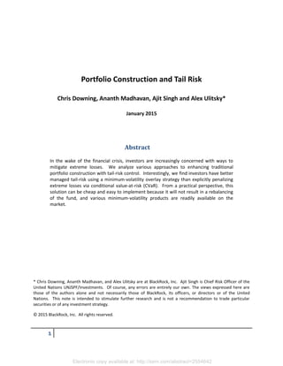
Figure 5 shows the finite-sample distributions of the Back-Test CVaR(5%) estimators and Figure 6 shows
the results for CVaR(1%) estimators. The distributions for each portfolio construction setup are
superimposed; as one moves from left to right on the horizontal axis, the weight on CVaR is increasing,
with the exception of MVol. First, it’s clear from Figure 5 and 6 that a CVaR penalty of sufficient
magnitude can make a meaningful reduction in out-of-sample CVaR performance for the alpha
portfolios. However, with 30 years of data the CVaR distributions are heavily overlapped. As a statistical
matter, we would reject the null hypothesis that the mean of the MV and Blend2 distribution are the
same, and similarly would reject the null of equality for Blend2 and Blend1, and for Blend1 and CVaR.
However, we do not reject the null that the mean CVaR of MCVaR and MVol (zero expected returns in
these two cases) are the same – at the 5% level with 30 years of data, we can’t distinguish the ex-post
portfolio CVaRs of these two optimization setups. For the 1% runs, the overlap is even more extreme,
so while statistically we might be able to distinguish the means, we have very little confidence in our
ability to distinguish these approaches in terms of their ex-post CVaRs with just 30 years of monthly
data.

16. 16
Figure 5: Finite-Sample Distributions of Back-Test CVaR(5%) Estimators
(Length of each back-test = 30 years, Number of back-tests = 100)
,
Figure 6: Finite-Sample Distributions of Back-Test CVaR(1%) Estimators
(Length of each back-test = 30 years, Number of back-tests = 100)
In summary, absent an alpha view, there is little difference between a minimum-CVaR and minimum-
Volatility (mean-variance) approach to portfolio construction, at least at the index level based on
simulations. Minimum volatility ETFs are available to investors in a variety of formats, offering a good
option for those seeking to mitigate tail risk in the context of a broadly diversified portfolio. We’ll return
to this issue below. In the presence of an alpha view, one must have a high degree of aversion to tail
risk before a tail-risk penalty will make sense in portfolio construction. As we saw above, unless we put
a relatively high weight on the CVaR penalty, the resulting out-of-sample portfolio CVaR will be difficult

17. 17
to distinguish from the CVaR of a mean-variance optimized portfolio. One needs to be willing to cut risk
significantly, and give up a fair amount of return, in order to make a reliable reduction in tail risk.
4. Security-Level Analysis
In the previous section, we used Monte Carlo analysis to illustrate that, in the absence of an alpha view,
the minimum-volatility portfolio has about the same (or better) ex-post CVaR performance than the
minimum-CVaR portfolio. We also showed that incorporating a tail-risk penalty into a conventional
mean-variance framework can reduce ex-post CVaR if enough weight is put on the tail risk penalty. In
part to test the robustness of these results, but also of interest in its own right, here we analyze a
variety of “bottom up,” or security-level, portfolio constructions for equity-only portfolios. First we
compare the minimum-volatility approach with minimum-CVaR, and a blended approach combining
penalties on total risk and CVaR. As a followup, we analyze the efficiency of minimum-volatility and
minimum-CVaR approaches in reducing ex-post CVaR for some common active strategies.
Minimum-Volatility and Minimum-CVaR for S&P500 and MSCI ACWI Index Strategies
Our empirical observations are based on historical back-test simulations for two different security
universes – MSCI ACWI and the S&P50012
. First, we consider the properties of minimum-volatility and
minimum-CVaR strategies. Similar to our Monte Carlo results, Table 5 shows that while the CVaR
penalty produces a reduction in ex-ante CVaR, on an ex-post basis the MinVol strategy results in a lower
CVaR for both universes13
.
Table 5: Ex-Post CVaRs
Panel A: S&P 500 Panel B: MSCI ACWI
Index MinVol MinCVaR
Risk 4.2 3.1 3.6
CVaR 9.6 7.1 7.9
VaR 7.3 4.9 5.8
Index MinVol MinCVaR
Risk 5.6 4.5 3.7
CVaR 12.8 7.3 9.9
VaR 9.3 4.8 6.4
These results underscore our previous results that historical CVaR estimates are not robust forecasts of
CVaR, and the MinVol strategy might be a better choice for tail-risk mitigation. The relatively poor ex-
post CVaR performance of the minimum-CVaR approach can be viewed as an analog to a well-known
12
Details of the simulations are in a technical appendix that is available upon request.
13
All numbers are expressed in monthly percents.

18. 18
fact that historic returns are not necessarily good predictors of future performance. One hypothesis on
the effectiveness of the minimum-volatility strategy in tail-risk mitigation is to recognize that a good
factor risk model incorporates significant amounts of asset- and firm-level information, in addition to
historical returns. The resulting model is parsimonious and, by being periodically re-estimated, it may
be a more accurate way to forecast tail risk.
To test this conjecture we repeat the above analysis for the S&P500, but we hold the risk model
unchanged throughout the back-test. In this simulation, the ex-post results for the MinVol strategy (last
column) are clearly inferior to minimum-CVaR, as shown in Table 6.
Table 6: Risk and Ex-Post CVaR for MinVol, MinCVaR, and Fixed-Risk Model MinVol
S&P500 MinVol MinCVaR MinVolFixedRisk
Risk 4.2 3.1 3.6 3.8
CVaR 9.6 7.1 7.9 8.5
To rationalize why our Monte Carlo results and the historical simulations above differ in terms of the
relative effectiveness of the MinCVaR and MinVol solutions at ex-post CVaR reduction, we can point to
the amount of available information. In the Monte Carlo simulations, the MinCVaR solution has the
ability to utilize an effectively unlimited amount of history. As we illustrated previously, this long history
was required for MinCVaR to dominate the MinVol strategy in terms of CVaR reduction. In practice, this
huge amount of historical information is never available.
Directly Constraining the Volatility Factor Exposure
Our second test explores whether direct constraints on the volatility factor exposure produce further
reductions in realized CVaR relative to the CVaR obtained under the standard minimum-volatility
strategy. To get a better understanding if this assertion would hold in bottom-up portfolio
constructions, we run a series of back-tests of the MinVol strategy on the S&P500 constituents, each
with a pre-determined upper bound on the volatility factor exposure of the resulting portfolio. Figure 7
illustrates effect of tightening the volatility factor exposure bounds, as one moves from right to left on
the horizontal axis, on ex-post CVaR, shown on the vertical axis.

19. 19
Figure 7: Influence of Constraint on Volatility Factor Exposure
The unconstrained MinVol portfolio has an absolute value of volatility exposure of about 0.7, so above
this value, the factor bound has no effect. When we limit the volatility exposure at 0.5, the resulting ex-
post CVAR monotonically increases, so this tail-reducing strategy does not play out.
Adding Tail-Risk Penalties to Mean-Variance Optimization
We next turn to consider some practical approaches to tail-risk mitigation. First, we consider the tail-
risk reduction achieved using total- versus tail-risk penalties in conventional mean-variance based
portfolio constructions. We analyze long-only portfolios, here tracking the MSCI ACWI equity index as a
benchmark.14
We run a horserace between the following two approaches:
1. Mean Variance with Tail Risk Penalty (CVaR)
][ TailRiskActiveRiskMinimize 
2. Mean Variance with Total Risk Penalty (TotVol)
][ TotalRiskActiveRiskMinimize 
To compare the effect of the penalty we run historic back-tests at different values of “ε”. Figures 8 and
9 show efficient frontiers computed on ex-ante and ex-post basis under the two approaches.
14
Details of the simulations are in a technical appendix available upon request.
0 0.5 1 1.5 2 2.5
7
7.5
8
8.5
Volatility Exposure Bounds
CVaR@5%(%)

20. 20
Figure 8: Ex-Ante Results for MSCI ACWI Figure 9: Ex-Post Results for MSCI ACWI
Similar to our results for individual MinVol and MinCVaR strategies, on an ex-ante basis the CVaR
penalty looks beneficial compared to the total volatility penalty. However, again the ex-post results
suggest that total volatility is actually the superior choice for tail-risk mitigation.
Note that, as shown below, adding the total volatility penalty helps to reduce tail-risk, but at the cost of
increasing tracking-error (active risk) relative to the benchmark:
Figure 10: Ex-Post Reults for MSCI ACWI
A cost-benefit analysis of adding Total Volatility penalty can be accomplished by, for example,
comparing the percent reduction in CVaR to the percent increase in percent tracking error (PTE). To
exploit this information, shown in Figure 11, we look for a blend offering a significant reduction in CVaR
with only modest increase in PTE. For example, blends 5 and 6 might warrant further analysis.
0 0.5 1 1.5 2 2.5 3 3.5 4 4.5 5
0
2
4
6
8
10
12
PTE (%)
CVaR(%)
CVaR
TotVol
MinVol/ACWV
MinCVaR
MinPTE/ACWI
0 0.5 1 1.5 2 2.5 3 3.5 4 4.5 5
6
7
8
9
10
11
12
13
14
PTE (%)
CVaR(%)
CVaR
TotVolMinPTE/ACWI
MinCVaR
MinVol/ACWV
0 1 2 3 4 5 6
6
7
8
9
10
11
12
13
14
PTE (%)
CVaR(%)
TotVolMinPTE
MinVol
Benefit = Reduction in CVaR
Cost = Increase in PTE

21. 21
Figure 11: Cost vs. Benefit for MSCI ACWI Case
Tail Risk and Some Popular Active Strategies
Finally, we focus on portfolios with an alpha view. Recently there has been significant interest in factor-
based portfolios. Here we study examples where the active strategy is expressed in terms of the value
and volatility style-factor portfolios. To carry out this analysis, we again use the S&P500 universe and
run historic back-tests using the Barra value factor exposure as the asset-level alpha. Figure 12 below
illustrates the influence of a CVaR penalty at a fixed alpha setting on realized risk and CVaR. Note that at
a fixed level of alpha, mean-variance optimization is reduced to the constrained minimum-volatility
portfolio construction. Therefore blending in an additional total-volatility penalty will not have any
effect on performance. In contrast, blending in the CVaR penalty with different weights will result in
different portfolios with different performance profiles, as illustrated below.
For the value factor a CVaR penalty does not provide any improvement in CVaR on ex-post basis.
Interestingly, even for the volatility factor there is only a small improvement in CVaR when tail-risk is
added into portfolio construction. This effect is stronger, however, if we consider how the CVaR penalty
influences ex-post tail risk further in the tail. The figure below illustrates, for two different levels of
expected alpha, how much CVaR at the 2% threshold is reduced when we add in a CVaR penalty based
on the 5% threshold (in other words, we measure ex-post CVaR further into the tail than the point at
which our optimization penalty is defined).
1 2 3 4 5 6
0
10
20
30
40
50
60
70
%
Increase in PTE
Reduction in CVaR
MinVol MinPTE

22. 22
Figure 12: Constrained Value Alpha, S&P 500 Backtest Using
Mean Variance and Blended Models with Increasing CVaR Influence
Panel A: Constrained Value Alpha (=1.27) Panel B: Constrained Value Alpha (=1.62)
Figure 13: Constrained Volatility Alpha (=3.25, 1.62), S&P 500 Backtest Using
Mean Variance and Blended Models with Increasing CVaR Influence.
Optimized at 5%, Reporting at 2%
The results in Figure 13 suggest that, at least for this active strategy, a CVaR penalty might provide some
ex-post tail-risk reduction relative to the total volatility penalty, but clearly more analysis has to be done
to reach any firm conclusions, given the wide confidence intervals around the CVaR estimators (not
shown but easily inferred from our Monte Carlo results).
5. Practical Approaches to Tail-Risk Mitigation
In practice, running even a blended model with a total risk penalty is fairly computationally complex. A
simple and cheap alternative is to overlay a minimum volatility strategy on the current portfolio. As
3.6 3.8 4 4.2 4.4 4.6 4.8 5
11.5
12
12.5
13
13.5
TE (%)
CVaR@2%(%)
Blend, a=3.25
Blend, a=1.62
3.6 3.7 3.8 3.9 4 4.1 4.2 4.3 4.4 4.5 4.6
9
9.5
10
10.5
11
11.5
12
TE (%)
CVaR(%)
MeanVar
Blend
Increase in CVaR Penalty
3.6 3.8 4 4.2 4.4 4.6
9
9.5
10
10.5
TE (%)
CVaR(%)
MeanVar
Blend

23. 23
shown in the table below, all of the minimum-volatility versions of popular equity indexes may offer
significant reductions in (ex-post) CVaR. This suggests that allocations to these minimum-volatility
exposures can be a cheap and easy way to reduce tail-risk.
Table 7: Reduction in Ex-Post CVaR
From a wider perspective, a tail-risk averse investor seeking to build a broadly diversified portfolio has
two main tools for tail-risk reduction. The first is an allocation into safer fixed-income instruments such
as government bonds, particularly short-dated bonds. Of course, this allocation typically comes at the
expense of expected return relative to a riskier allocation – there is no free lunch even in tail-risk
reduction. The second tool for tail-risk reduction is a minimum-volatility equity exposure in the equity
sleeve.
To get a feel for the 1% and 5% CVaRs that have been delivered by different allocations into US equities
and bonds, the table below provides some summary statistics for portfolios constructed from ETFs
tracking the Barclays Aggregate Bond Index (AGG), the S&P500 (IVV) and the MSCI USA index (EUSA), .
The top panels shows summary statistics for monthly and daily returns on the individual ETFs, and the
lower panel shows statistics for portfolios allocated 60% into the indicated equity exposure, and 40%
into AGG.
As can be seen in the table below, diversifying into bonds provides the most significant reduction in tail
risk with some reduction in average total return.
Standard Index Min Vol Index
MSCI ACWI -11.5 -8.2 29%
MSCI ACWI ex US -12.8 -8.5 34%
MSCI World -11.3 -8.6 24%
MSCI US -10.3 -8.8 15%
MSCI EAFE -12.6 -8.9 29%
MSCI EM -14.9 -11.8 20%
CVaR (5%) % Reduction in Ex-
Post CVaR (5%)

24. 24
Table 8: Summary Statistics
January 1999 – October 201415
6. Conclusions
We examined approaches to enhancing traditional mean-variance portfolio construction with tail-risk
control. We analyzed tail-risk control in the context of conditional value-at-risk, a measure that is
intuitive and easy to compute, and that offers some attractive statistical properties. A consistent result
is that minimum-volatility constructions are competitive with minimum-CVaR in mitigating tail-risk
exposure. We attribute this to the fact that minimum-volatility approaches leverage factor risk models
that incorporate a lot of information beyond historical returns, and update the risk estimates regularly,
while CVaR calculations only update on infrequent tail events. Indeed, we found that if we hold our risk
model static, minimum-CVaR portfolios can “beat” minimum-volatility portfolios in terms of ex-post
CVaR, at least over the period we study. In the alpha context, we found largely the same result, at least
for the two active strategies we analyzed (volatility and value factor portfolios). Finally, we examined
the degree to which an investor can potentially mitigate tail risk in a broadly diversified multi-asset
portfolio by blending in minimum-volatility exposures. Combining broad fixed-income exposures and
minimum-volatility equity exposures, investors can cheaply and effectively mitigate tail-risk exposure.
15
ETF NAV-based total returns are used where available, and funds’ underlying index returns are used for the period prior to
the ETFs’ inception. The following index returns are used prior to the fund’s inception: for AGG: Barclays US Aggregate Bond
Index, for IVV: S&P 500 Index and for EUSA: MSCI USA Index.
Ticker Summary
Ticker Return Vol CVaR(5%) CVaR(1%) Max(drawdown)
Monthly Returns
AGG 0.0511 0.0353 -0.0195 -0.0301 -0.0336
IVV 0.0586 0.1518 -0.0970 -0.1381 -0.1677
EUSA 0.0583 0.1531 -0.0966 -0.1419 -0.1710
Daily Returns
AGG 0.0496 0.0378 -0.0053 -0.0075 -0.0118
IVV 0.0656 0.1998 -0.0298 -0.0495 -0.0901
EUSA 0.0651 0.2002 -0.0298 -0.0494 -0.0907
Portfolio Summary
Portfolio Return Vol CVaR(5%) CVaR(1%) Max(drawdown)
Monthly Returns
AGG/IVV 0.0556 0.0909 -0.0579 -0.0873 -0.1093
AGG/EUSA 0.0554 0.0916 -0.0577 -0.0872 -0.1113
Daily Returns
AGG/IVV 0.0601 0.1181 -0.0171 -0.0290 -0.0537
AGG/EUSA 0.0599 0.1183 -0.0171 -0.0289 -0.0541

25. 25
Standardized Performance as of 12/31/2014
Fund Name
Fund
Inception
Date
Gross
Exp.
Ratio
30-Day SEC
Yield (With/
Without
Waiver)
Contractual
Fee Waiver
Expiration (If
Applicable) 1-Year 5-Year 10-Year
Since
Inception
iShares Core U.S. Treasury Bond ETF (GOVT) 2/14/12 0.15% 1.28% --
Fund NAV Total Return 4.99% -- -- 1.40%
Fund Market Price Total Return 4.98% -- -- 1.44%
Index Total Return 5.05% 3.91% 4.38% 1.49%
iShares Core U.S. Credit Bond ETF (CRED) 1/5/07 0.15% 2.89% --
Fund NAV Total Return 7.37% 6.03% -- 5.75%
Fund Market Price Total Return 8.00% 6.06% -- 5.78%
Index Total Return 7.53% 6.25% 5.46% 6.01%
iShares Core S&P 500 ETF (IVV) 5/15/00 0.07% 2.04% --
Fund NAV Total Return 13.62% 15.37% 7.62% 4.33%
Fund Market Price Total Return 13.62% 15.38% 7.62% 4.33%
Index Total Return 13.69% 15.45% 7.67% 4.40%
iShares MSCI Emerging Markets ETF (EEM) 4/7/03 0.68% 2.03% 12/31/15
Fund NAV Total Return -2.82% 0.76% 7.70% 13.08%
Fund Market Price Total Return -3.98% 0.85% 7.64% 13.08%
Index Total Return -2.19% 1.78% 8.43% 13.52%
iShares MSCI USA ETF (EUSA) 5/5/10 0.15% 1.92% --
Fund NAV Total Return 13.20% -- -- 15.27%
Fund Market Price Total Return 13.31% -- -- 15.28%
Index Total Return 13.36% 15.50% 7.82% 15.49%
iShares Core U.S. Aggregate Bond ETF (AGG) 9/22/03 0.09% 1.91%/1.90% 6/30/15
Fund NAV Total Return 6.04% 4.30% 4.53% 4.52%
Fund Market Price Total Return 6.01% 4.33% 4.51% 4.53%
Index Total Return 5.97% 4.45% 4.71% 4.71%
The performance quoted represents past performance and does not guarantee future results.
Investment return and principal value of an investment will fluctuate so that an investor’s shares,
when sold or redeemed, may be worth more or less than the original cost. Current performance may
be lower or higher than the performance quoted. Performance data current to the most recent month
end may be obtained by visiting www.iShares.com or www.blackrock.com. Shares of ETFs are bought
and sold at market price (not NAV) and are not individually redeemed from the Fund. Brokerage
commissions will reduce returns. Market returns are based upon the midpoint of the bid/ask spread at
4:00 p.m. eastern time (when NAV is normally determined for most ETFs), and do not represent the
returns you would receive if you traded shares at other times.
Carefully consider the Funds' investment objectives, risk factors, and charges and expenses before
investing. This and other information can be found in the Funds' prospectuses or, if available, the
summary prospectuses which may be obtained by visiting www.iShares.com or www.blackrock.com.
Read the prospectus carefully before investing.

26. 26
Index returns are for illustrative purposes only. Index performance returns do not reflect any management fees,
transaction costs or expenses. Indexes are unmanaged and one cannot invest directly in an index. Past
performance does not guarantee future results.
Investing involves risk, including possible loss of principal.The iShares Minimum Volatility ETFs may experience
more than minimum volatility as there is no guarantee that the underlying index's strategy of seeking to lower
volatility will be successful.
This material is not intended to be relied upon as a forecast, research or investment advice, and is not a
recommendation, offer or solicitation to buy or sell any securities or to adopt any investment strategy. The
opinions expressed are those of the authors, and may change as subsequent conditions vary. Individual portfolio
managers for BlackRock may have opinions and/or make investment decisions that, in certain respects, may not be
consistent with the information contained in this document. The information and opinions contained in this
material are derived from proprietary and nonproprietary sources deemed by BlackRock to be reliable, are not
necessarily all-inclusive and are not guaranteed as to accuracy. Past performance is no guarantee of future results.
There is no guarantee that any forecasts made will come to pass. Reliance upon information in this material is at
the sole discretion of the reader.
The Funds are distributed by BlackRock Investments, LLC (together with its affiliates, “BlackRock”).
The iShares Funds are not sponsored, endorsed, issued, sold or promoted by MSCI Inc. or S&P Dow Jones Indices
LLC. Neither of these companies make any representation regarding the advisability of investing in the Funds.
BlackRock is not affiliated with the companies listed above.
©2014 BlackRock, Inc. All rights reserved. iSHARES and BLACKROCK are registered trademarks of BlackRock, Inc.,
or its subsidiaries. All other marks are the property of their respective owners. iS-14188-1214