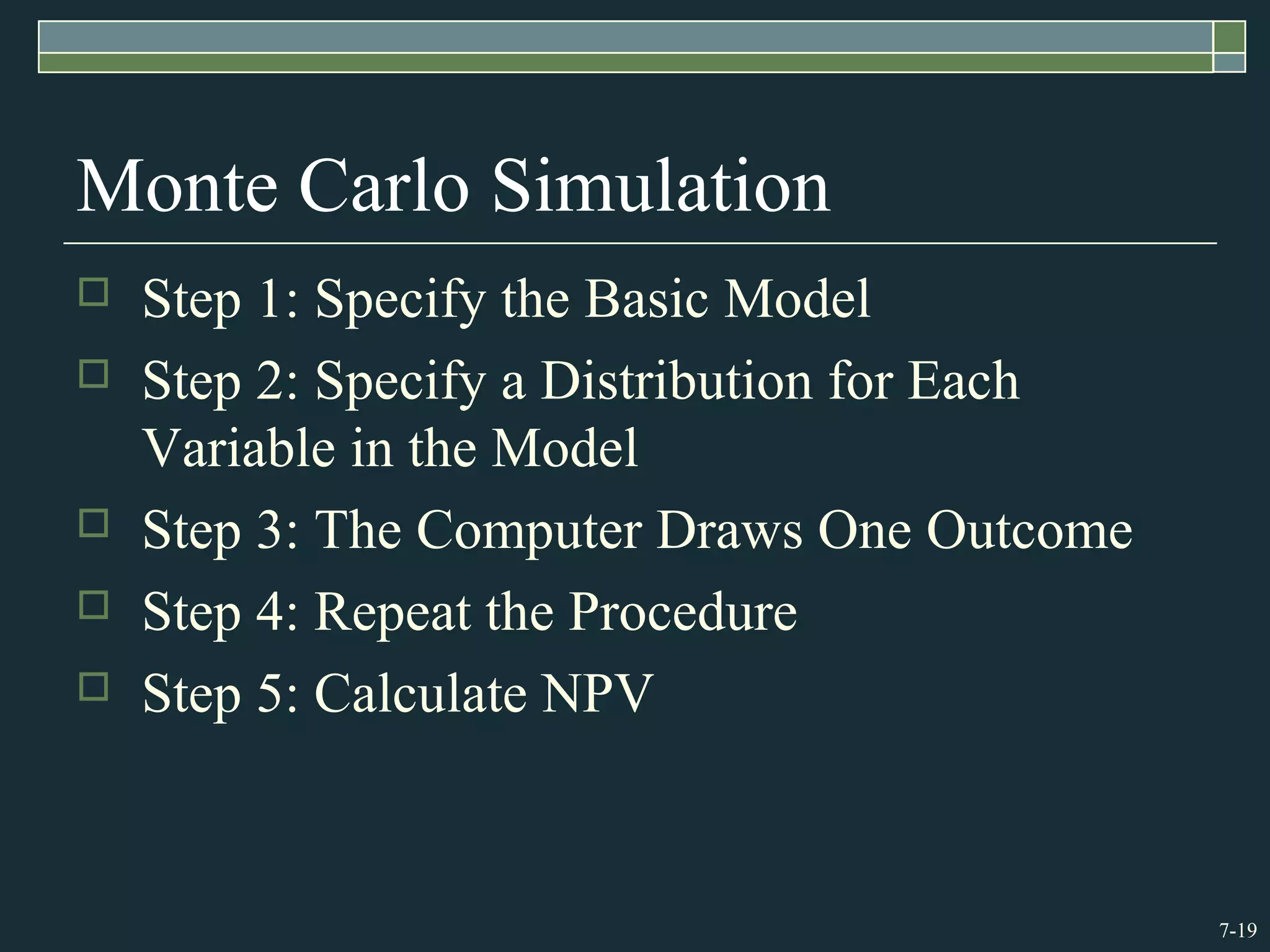
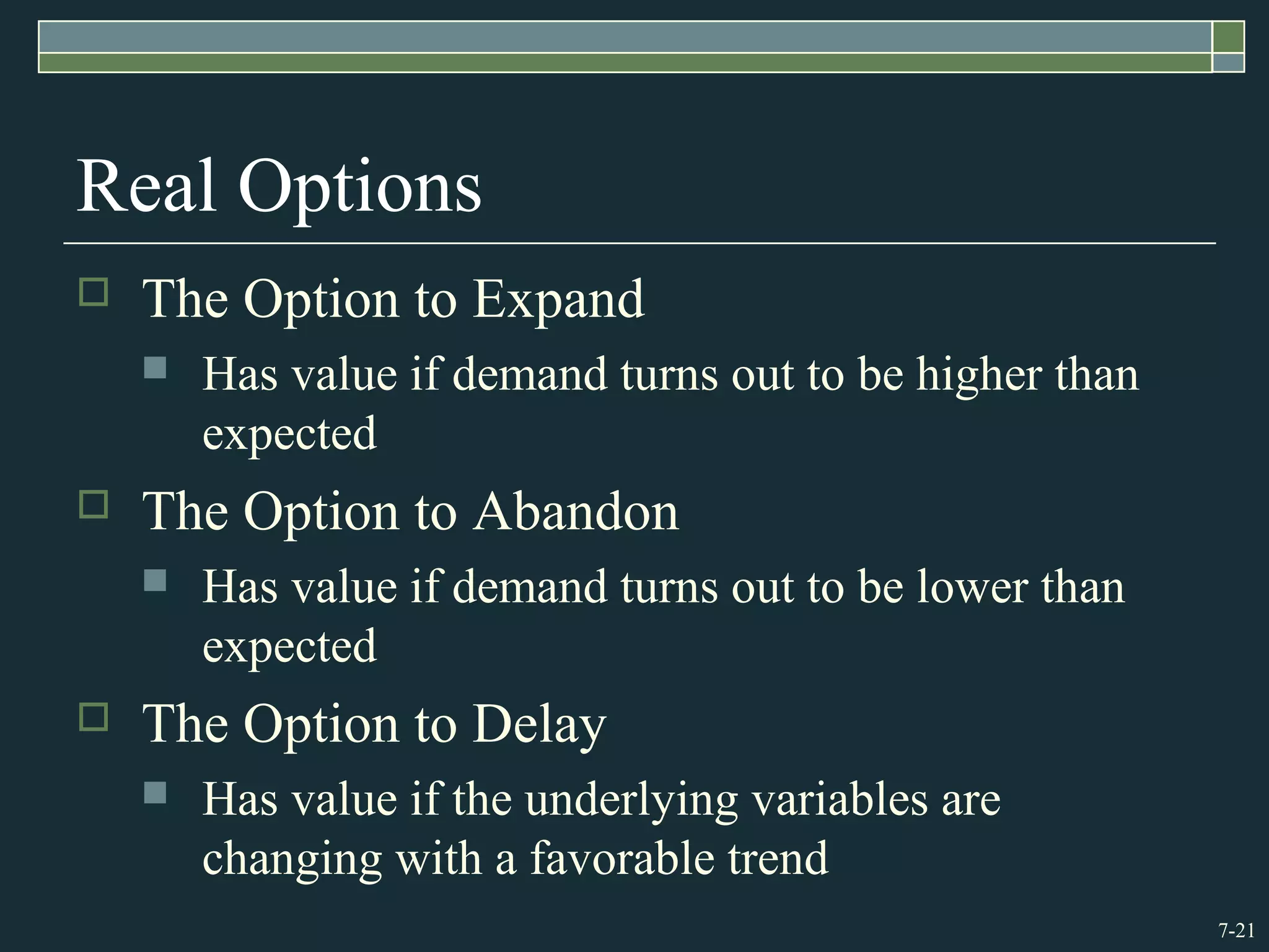
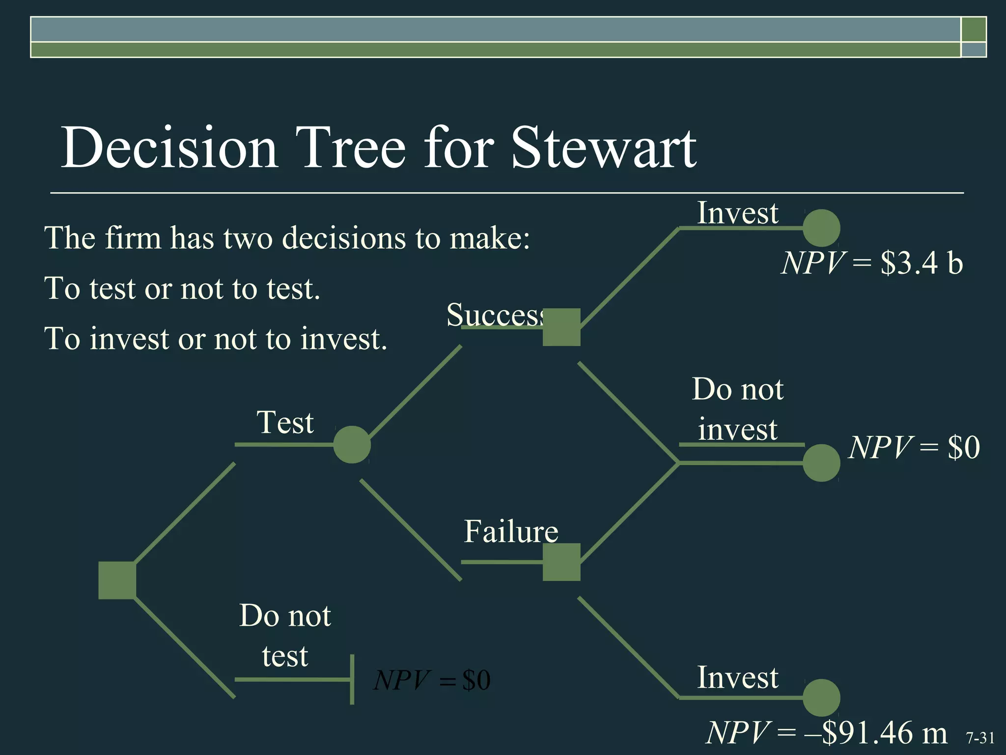
Risk Analysis, Real Options, and Capital
Budgeting
Chapter 7
Copyright © 2010 by the McGraw-Hill Companies, Inc. All rights reserved.McGraw-Hill/Irwin
7-2
Key Concepts and Skills
 Understand and be able to apply scenario and
sensitivity analysis
 Understand the various forms of break-even
analysis
 Understand Monte Carlo simulation
 Understand the importance of real options in
capital budgeting
 Understand decision trees
7-3
Chapter Outline
7.1 Sensitivity Analysis, Scenario Analysis,
and Break-Even Analysis
7.2 Monte Carlo Simulation
7.3 Real Options
7.4 Decision Trees
7-4
7.1 Sensitivity, Scenario, and Break-Even
 Each allows us to look behind the NPV
number to see how stable our estimates
are.
 When working with spreadsheets, try to
build your model so that you can adjust
variables in a single cell and have the
NPV calculations update accordingly.
7-5
Example: Stewart Pharmaceuticals
 Stewart Pharmaceuticals Corporation is considering investing
in the development of a drug that cures the common cold.
 A corporate planning group, including representatives from
production, marketing, and engineering, has recommended
that the firm go ahead with the test and development phase.
 This preliminary phase will last one year and cost $1 billion.
Furthermore, the group believes that there is a 60% chance
that tests will prove successful.
 If the initial tests are successful, Stewart Pharmaceuticals can
go ahead with full-scale production. This investment phase
will cost $1.6 billion. Production will occur over the
following 4 years.
7-6
NPV Following Successful Test
Note that the NPV is
calculated as of date 1, the
date at which the
investment of $1,600
million is made. Later we
bring this number back to
date 0. Assume a cost of
capital of 10%.
Investment Year 1 Years 2-5
Revenues $7,000
Variable Costs (3,000)
Fixed Costs (1,800)
Depreciation (400)
Pretax profit $1,800
Tax (34%) (612)
Net Profit $1,188
Cash Flow -$1,600 $1,588
75.433,3$
)10.1(
588,1$
600,1$
1
4
1
1
=
+−= ∑=
NPV
NPV
t
t
7-7
NPV Following Unsuccessful Test
Note that the NPV is
calculated as of date 1,
the date at which the
investment of $1,600
million is made. Later
we bring this number
back to date 0. Assume a
cost of capital of 10%.
Investment Year 1 Years 2-5
Revenues $4,050
Variable Costs (1,735)
Fixed Costs (1,800)
Depreciation (400)
Pretax profit $115
Tax (34%) (39.10)
Net Profit $75.90
Cash Flow -$1,600 $475.90
461.91$
)10.1(
90.475$
600,1$
1
4
1
1
−=
+−= ∑=
NPV
NPV
t
t
7-8
Decision to Test
 Let’s move back to the first stage, where the decision boils
down to the simple question: should we invest?
 The expected payoff evaluated at date 1 is:






×+





×=
failuregiven
Payoff
failure
Prob.
successgiven
Payoff
sucess
Prob.
payoff
Expected
( ) ( ) 25.060,2$0$40.75.433,3$60.
payoff
Expected
=×+×=
95.872$
10.1
25.060,2$
000,1$ =+−=NPV
The NPV evaluated at date 0 is:
So, we should test.
7-9
Sensitivity Analysis: Stewart
%29.14
000,7$
000,7$000,6$
Rev% −=
−
=∆
 We can see that NPV is very sensitive to changes in revenues.
In the Stewart Pharmaceuticals example, a 14% drop in
revenue leads to a 61% drop in NPV.
%93.60
75.433,3$
75.433,3$64.341,1$
% −=
−
=∆NPV
For every 1% drop in revenue, we can expect roughly a
4.26% drop in NPV:
%29.14
%93.60
26.4
−
=−
7-10
Scenario Analysis: Stewart
 A variation on sensitivity analysis is scenario analysis.
 For example, the following three scenarios could apply
to Stewart Pharmaceuticals:
1. The next few years each have heavy cold seasons, and
sales exceed expectations, but labor costs skyrocket.
2. The next few years are normal, and sales meet
expectations.
3. The next few years each have lighter than normal cold
seasons, so sales fail to meet expectations.
 Other scenarios could apply to FDA approval.
 For each scenario, calculate the NPV.
7-11
Break-Even Analysis
 Common tool for analyzing the relationship
between sales volume and profitability
 There are three common break-even measures
 Accounting break-even: sales volume at which net
income = 0
 Cash break-even: sales volume at which operating
cash flow = 0
 Financial break-even: sales volume at which net
present value = 0
7-12
Break-Even Analysis: Stewart
 Another way to examine variability in
our forecasts is break-even analysis.
 In the Stewart Pharmaceuticals example,
we could be concerned with break-even
revenue, break-even sales volume, or
break-even price.
 To find either, we start with the break-
even operating cash flow.
7-13
Break-Even Analysis: Stewart
 The project requires an
investment of $1,600.
 In order to cover our cost
of capital (break even), the
project needs to generate a
cash flow of $504.75 each
year for four years.
 This is the project’s break-
even operating cash flow,
OCFBE.
PMT
I/Y
FV
PV
N
− 504.75
10
0
1,600
4
PV
7-14
Break-Even Revenue: Stewart
Work backwards from OCFBE to Break-Even Revenue
Revenue $5,358.71
Variable cost $3,000
Fixed cost $1,800
Depreciation $400
EBIT $158.71
Tax (34%) $53.96
Net Income $104.75
OCF = $104.75 + $400 $504.75
$104.75
0.66
+D
+FC
+ VC
7-15
Break-Even Analysis: PBE
 Now that we have break-even revenue of $5,358.71
million, we can calculate break-even price.
 The original plan was to generate revenues of $7
billion by selling the cold cure at $10 per dose and
selling 700 million doses per year,
 We can reach break-even revenue with a price of
only:
$5,358.71 million = 700 million × PBE
PBE = = $7.66 / dose
700
$5,358.71
7-16
7.2 Monte Carlo Simulation
 Monte Carlo simulation is a further
attempt to model real-world uncertainty.
 This approach takes its name from the
famous European casino, because it
analyzes projects the way one might
evaluate gambling strategies.
7-17
Monte Carlo Simulation
 Imagine a serious blackjack player who wants to
know if she should take the third card whenever her
first two cards total sixteen.
 She could play thousands of hands for real money to
find out.
 This could be hazardous to her wealth.
 Or, she could play thousands of practice hands.
 Monte Carlo simulation of capital budgeting projects
is in this spirit.
7-18
Monte Carlo Simulation
 Monte Carlo simulation of capital budgeting projects
is often viewed as a step beyond either sensitivity
analysis or scenario analysis.
 Interactions between the variables are explicitly
specified in Monte Carlo simulation; so, at least
theoretically, this methodology provides a more
complete analysis.
 While the pharmaceutical industry has pioneered
applications of this methodology, its use in other
industries is far from widespread.
7-19
Monte Carlo Simulation
 Step 1: Specify the Basic Model
 Step 2: Specify a Distribution for Each
Variable in the Model
 Step 3: The Computer Draws One Outcome
 Step 4: Repeat the Procedure
 Step 5: Calculate NPV
7-20
7.3 Real Options
 One of the fundamental insights of modern
finance theory is that options have value.
 The phrase “We are out of options” is surely a
sign of trouble.
 Because corporations make decisions in a
dynamic environment, they have options that
should be considered in project valuation.
7-21
Real Options
 The Option to Expand
 Has value if demand turns out to be higher than
expected
 The Option to Abandon
 Has value if demand turns out to be lower than
expected
 The Option to Delay
 Has value if the underlying variables are
changing with a favorable trend
7-22
Discounted CF and Options
 We can calculate the market value of a project as the
sum of the NPV of the project without options and
the value of the managerial options implicit in the
project.
M = NPV + Opt
A good example would be comparing the desirability
of a specialized machine versus a more versatile
machine. If they both cost about the same and last
the same amount of time, the more versatile machine
is more valuable because it comes with options.
7-23
The Option to Abandon: Example
 Suppose we are drilling an oil well. The
drilling rig costs $300 today, and in one year
the well is either a success or a failure.
 The outcomes are equally likely. The
discount rate is 10%.
 The PV of the successful payoff at time one
is $575.
 The PV of the unsuccessful payoff at time
one is $0.
7-24
The Option to Abandon: Example
Traditional NPV analysis would indicate rejection of the project.
NPV = = –$38.64
1.10
$287.50
–$300 +
Expected
Payoff
= (0.50×$575) + (0.50×$0) = $287.50
=Expected
Payoff
Prob.
Success
×Successful
Payoff
+ Prob.
Failure
× Failure
Payoff
7-25
The Option to Abandon: Example
The firm has two decisions to make: drill or not, abandon or stay.
Do not
drill
Drill
0$=NPV
500$−
Failure
Success: PV = $500
Sell the rig;
salvage value
= $250
Sit on rig; stare
at empty hole:
PV = $0.
However, traditional NPV analysis overlooks the option to abandon.
7-26
The Option to Abandon: Example
 When we include the value of the option to abandon,
the drilling project should proceed:
NPV = = $75.00
1.10
$412.50
–$300 +
Expected
Payoff
= (0.50×$575) + (0.50×$250) = $412.50
=Expected
Payoff
Prob.
Success
×Successful
Payoff
+ Prob.
Failure
× Failure
Payoff
7-27
Valuing the Option to Abandon
 Recall that we can calculate the market value of a
project as the sum of the NPV of the project
without options and the value of the managerial
options implicit in the project.
M = NPV + Opt
$75.00 = –$38.64 + Opt
$75.00 + $38.64 = Opt
Opt = $113.64
7-28
The Option to Delay: Example
 Consider the above project, which can be undertaken in any
of the next 4 years. The discount rate is 10 percent. The
present value of the benefits at the time the project is
launched remains constant at $25,000, but since costs are
declining, the NPV at the time of launch steadily rises.
 The best time to launch the project is in year 2—this schedule
yields the highest NPV when judged today.
Year Cost PV NPV t
0 20,000$ 25,000$ 5,000$
1 18,000$ 25,000$ 7,000$
2 17,100$ 25,000$ 7,900$
3 16,929$ 25,000$ 8,071$
4 16,760$ 25,000$ 8,240$
2
)10.1(
900,7$
529,6$ =
Year Cost PV NPV t NPV 0
0 20,000$ 25,000$ 5,000$ 5,000$
1 18,000$ 25,000$ 7,000$ 6,364$
2 17,100$ 25,000$ 7,900$ 6,529$
3 16,929$ 25,000$ 8,071$ 6,064$
4 16,760$ 25,000$ 8,240$ 5,628$
7-29
7.4 Decision Trees
 Allow us to graphically represent the
alternatives available to us in each period
and the likely consequences of our
actions
 This graphical representation helps to
identify the best course of action.
7-30
Example of a Decision Tree
Do not
study
Study
finance
Squares represent decisions to be made. Circles represent
receipt of information,
e.g., a test score.
The lines leading away
from the squares
represent the alternatives.
“C”
“A”
“B”
“F”
“D”
7-31
Decision Tree for Stewart
Do not
test
Test
Failure
Success
Do not
invest
Invest
Invest
The firm has two decisions to make:
To test or not to test.
To invest or not to invest.
0$=NPV
NPV = $3.4 b
NPV = $0
NPV = –$91.46 m
7-32
Quick Quiz
 What are sensitivity analysis, scenario
analysis, break-even analysis, and simulation?
 Why are these analyses important, and how
should they be used?
 How do real options affect the value of capital
projects?
 What information does a decision tree
provide?

Chap007

  • 1.
    Risk Analysis, RealOptions, and Capital Budgeting Chapter 7 Copyright © 2010 by the McGraw-Hill Companies, Inc. All rights reserved.McGraw-Hill/Irwin
  • 2.
    7-2 Key Concepts andSkills  Understand and be able to apply scenario and sensitivity analysis  Understand the various forms of break-even analysis  Understand Monte Carlo simulation  Understand the importance of real options in capital budgeting  Understand decision trees
  • 3.
    7-3 Chapter Outline 7.1 SensitivityAnalysis, Scenario Analysis, and Break-Even Analysis 7.2 Monte Carlo Simulation 7.3 Real Options 7.4 Decision Trees
  • 4.
    7-4 7.1 Sensitivity, Scenario,and Break-Even  Each allows us to look behind the NPV number to see how stable our estimates are.  When working with spreadsheets, try to build your model so that you can adjust variables in a single cell and have the NPV calculations update accordingly.
  • 5.
    7-5 Example: Stewart Pharmaceuticals Stewart Pharmaceuticals Corporation is considering investing in the development of a drug that cures the common cold.  A corporate planning group, including representatives from production, marketing, and engineering, has recommended that the firm go ahead with the test and development phase.  This preliminary phase will last one year and cost $1 billion. Furthermore, the group believes that there is a 60% chance that tests will prove successful.  If the initial tests are successful, Stewart Pharmaceuticals can go ahead with full-scale production. This investment phase will cost $1.6 billion. Production will occur over the following 4 years.
  • 6.
    7-6 NPV Following SuccessfulTest Note that the NPV is calculated as of date 1, the date at which the investment of $1,600 million is made. Later we bring this number back to date 0. Assume a cost of capital of 10%. Investment Year 1 Years 2-5 Revenues $7,000 Variable Costs (3,000) Fixed Costs (1,800) Depreciation (400) Pretax profit $1,800 Tax (34%) (612) Net Profit $1,188 Cash Flow -$1,600 $1,588 75.433,3$ )10.1( 588,1$ 600,1$ 1 4 1 1 = +−= ∑= NPV NPV t t
  • 7.
    7-7 NPV Following UnsuccessfulTest Note that the NPV is calculated as of date 1, the date at which the investment of $1,600 million is made. Later we bring this number back to date 0. Assume a cost of capital of 10%. Investment Year 1 Years 2-5 Revenues $4,050 Variable Costs (1,735) Fixed Costs (1,800) Depreciation (400) Pretax profit $115 Tax (34%) (39.10) Net Profit $75.90 Cash Flow -$1,600 $475.90 461.91$ )10.1( 90.475$ 600,1$ 1 4 1 1 −= +−= ∑= NPV NPV t t
  • 8.
    7-8 Decision to Test Let’s move back to the first stage, where the decision boils down to the simple question: should we invest?  The expected payoff evaluated at date 1 is:       ×+      ×= failuregiven Payoff failure Prob. successgiven Payoff sucess Prob. payoff Expected ( ) ( ) 25.060,2$0$40.75.433,3$60. payoff Expected =×+×= 95.872$ 10.1 25.060,2$ 000,1$ =+−=NPV The NPV evaluated at date 0 is: So, we should test.
  • 9.
    7-9 Sensitivity Analysis: Stewart %29.14 000,7$ 000,7$000,6$ Rev%−= − =∆  We can see that NPV is very sensitive to changes in revenues. In the Stewart Pharmaceuticals example, a 14% drop in revenue leads to a 61% drop in NPV. %93.60 75.433,3$ 75.433,3$64.341,1$ % −= − =∆NPV For every 1% drop in revenue, we can expect roughly a 4.26% drop in NPV: %29.14 %93.60 26.4 − =−
  • 10.
    7-10 Scenario Analysis: Stewart A variation on sensitivity analysis is scenario analysis.  For example, the following three scenarios could apply to Stewart Pharmaceuticals: 1. The next few years each have heavy cold seasons, and sales exceed expectations, but labor costs skyrocket. 2. The next few years are normal, and sales meet expectations. 3. The next few years each have lighter than normal cold seasons, so sales fail to meet expectations.  Other scenarios could apply to FDA approval.  For each scenario, calculate the NPV.
  • 11.
    7-11 Break-Even Analysis  Commontool for analyzing the relationship between sales volume and profitability  There are three common break-even measures  Accounting break-even: sales volume at which net income = 0  Cash break-even: sales volume at which operating cash flow = 0  Financial break-even: sales volume at which net present value = 0
  • 12.
    7-12 Break-Even Analysis: Stewart Another way to examine variability in our forecasts is break-even analysis.  In the Stewart Pharmaceuticals example, we could be concerned with break-even revenue, break-even sales volume, or break-even price.  To find either, we start with the break- even operating cash flow.
  • 13.
    7-13 Break-Even Analysis: Stewart The project requires an investment of $1,600.  In order to cover our cost of capital (break even), the project needs to generate a cash flow of $504.75 each year for four years.  This is the project’s break- even operating cash flow, OCFBE. PMT I/Y FV PV N − 504.75 10 0 1,600 4 PV
  • 14.
    7-14 Break-Even Revenue: Stewart Workbackwards from OCFBE to Break-Even Revenue Revenue $5,358.71 Variable cost $3,000 Fixed cost $1,800 Depreciation $400 EBIT $158.71 Tax (34%) $53.96 Net Income $104.75 OCF = $104.75 + $400 $504.75 $104.75 0.66 +D +FC + VC
  • 15.
    7-15 Break-Even Analysis: PBE Now that we have break-even revenue of $5,358.71 million, we can calculate break-even price.  The original plan was to generate revenues of $7 billion by selling the cold cure at $10 per dose and selling 700 million doses per year,  We can reach break-even revenue with a price of only: $5,358.71 million = 700 million × PBE PBE = = $7.66 / dose 700 $5,358.71
  • 16.
    7-16 7.2 Monte CarloSimulation  Monte Carlo simulation is a further attempt to model real-world uncertainty.  This approach takes its name from the famous European casino, because it analyzes projects the way one might evaluate gambling strategies.
  • 17.
    7-17 Monte Carlo Simulation Imagine a serious blackjack player who wants to know if she should take the third card whenever her first two cards total sixteen.  She could play thousands of hands for real money to find out.  This could be hazardous to her wealth.  Or, she could play thousands of practice hands.  Monte Carlo simulation of capital budgeting projects is in this spirit.
  • 18.
    7-18 Monte Carlo Simulation Monte Carlo simulation of capital budgeting projects is often viewed as a step beyond either sensitivity analysis or scenario analysis.  Interactions between the variables are explicitly specified in Monte Carlo simulation; so, at least theoretically, this methodology provides a more complete analysis.  While the pharmaceutical industry has pioneered applications of this methodology, its use in other industries is far from widespread.
  • 19.
    7-19 Monte Carlo Simulation Step 1: Specify the Basic Model  Step 2: Specify a Distribution for Each Variable in the Model  Step 3: The Computer Draws One Outcome  Step 4: Repeat the Procedure  Step 5: Calculate NPV
  • 20.
    7-20 7.3 Real Options One of the fundamental insights of modern finance theory is that options have value.  The phrase “We are out of options” is surely a sign of trouble.  Because corporations make decisions in a dynamic environment, they have options that should be considered in project valuation.
  • 21.
    7-21 Real Options  TheOption to Expand  Has value if demand turns out to be higher than expected  The Option to Abandon  Has value if demand turns out to be lower than expected  The Option to Delay  Has value if the underlying variables are changing with a favorable trend
  • 22.
    7-22 Discounted CF andOptions  We can calculate the market value of a project as the sum of the NPV of the project without options and the value of the managerial options implicit in the project. M = NPV + Opt A good example would be comparing the desirability of a specialized machine versus a more versatile machine. If they both cost about the same and last the same amount of time, the more versatile machine is more valuable because it comes with options.
  • 23.
    7-23 The Option toAbandon: Example  Suppose we are drilling an oil well. The drilling rig costs $300 today, and in one year the well is either a success or a failure.  The outcomes are equally likely. The discount rate is 10%.  The PV of the successful payoff at time one is $575.  The PV of the unsuccessful payoff at time one is $0.
  • 24.
    7-24 The Option toAbandon: Example Traditional NPV analysis would indicate rejection of the project. NPV = = –$38.64 1.10 $287.50 –$300 + Expected Payoff = (0.50×$575) + (0.50×$0) = $287.50 =Expected Payoff Prob. Success ×Successful Payoff + Prob. Failure × Failure Payoff
  • 25.
    7-25 The Option toAbandon: Example The firm has two decisions to make: drill or not, abandon or stay. Do not drill Drill 0$=NPV 500$− Failure Success: PV = $500 Sell the rig; salvage value = $250 Sit on rig; stare at empty hole: PV = $0. However, traditional NPV analysis overlooks the option to abandon.
  • 26.
    7-26 The Option toAbandon: Example  When we include the value of the option to abandon, the drilling project should proceed: NPV = = $75.00 1.10 $412.50 –$300 + Expected Payoff = (0.50×$575) + (0.50×$250) = $412.50 =Expected Payoff Prob. Success ×Successful Payoff + Prob. Failure × Failure Payoff
  • 27.
    7-27 Valuing the Optionto Abandon  Recall that we can calculate the market value of a project as the sum of the NPV of the project without options and the value of the managerial options implicit in the project. M = NPV + Opt $75.00 = –$38.64 + Opt $75.00 + $38.64 = Opt Opt = $113.64
  • 28.
    7-28 The Option toDelay: Example  Consider the above project, which can be undertaken in any of the next 4 years. The discount rate is 10 percent. The present value of the benefits at the time the project is launched remains constant at $25,000, but since costs are declining, the NPV at the time of launch steadily rises.  The best time to launch the project is in year 2—this schedule yields the highest NPV when judged today. Year Cost PV NPV t 0 20,000$ 25,000$ 5,000$ 1 18,000$ 25,000$ 7,000$ 2 17,100$ 25,000$ 7,900$ 3 16,929$ 25,000$ 8,071$ 4 16,760$ 25,000$ 8,240$ 2 )10.1( 900,7$ 529,6$ = Year Cost PV NPV t NPV 0 0 20,000$ 25,000$ 5,000$ 5,000$ 1 18,000$ 25,000$ 7,000$ 6,364$ 2 17,100$ 25,000$ 7,900$ 6,529$ 3 16,929$ 25,000$ 8,071$ 6,064$ 4 16,760$ 25,000$ 8,240$ 5,628$
  • 29.
    7-29 7.4 Decision Trees Allow us to graphically represent the alternatives available to us in each period and the likely consequences of our actions  This graphical representation helps to identify the best course of action.
  • 30.
    7-30 Example of aDecision Tree Do not study Study finance Squares represent decisions to be made. Circles represent receipt of information, e.g., a test score. The lines leading away from the squares represent the alternatives. “C” “A” “B” “F” “D”
  • 31.
    7-31 Decision Tree forStewart Do not test Test Failure Success Do not invest Invest Invest The firm has two decisions to make: To test or not to test. To invest or not to invest. 0$=NPV NPV = $3.4 b NPV = $0 NPV = –$91.46 m
  • 32.
    7-32 Quick Quiz  Whatare sensitivity analysis, scenario analysis, break-even analysis, and simulation?  Why are these analyses important, and how should they be used?  How do real options affect the value of capital projects?  What information does a decision tree provide?

Editor's Notes

  • #9 Note that we use the initial testing cost of $1 B, as the production costs were already applied in finding the payoffs.
  • #10 The calculations assume that revenues change as a result of a reduction in sales price; therefore, variable costs are unchanged. If revenue drops as a result of units, then the NPV is $2,239, which is a drop of 35%.
  • #11 Note the irony of scenario 1: our workers are too sick to make the medicine. Scenario analysis is often commonly employed by identifying the best and worst possible cases of all variables.
  • #14 This example looks purely at the project once the decision to invest has been made, making the initial $1 B a sunk cost.
  • #29 NPV0 = NPVt / (1.10)t
  • #32 If you don’t invest, the NPV = 0, even if you test first, because the cost of testing becomes a sunk cost. If you are so unwise as to invest in the face of a failed test, you incur lots of additional costs, but not much in the way of revenue, so you have a negative NPV as of date 1. Referring back to slide 7 (Decision to Test) may help to clarify the application of decision trees.