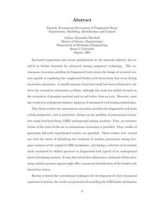
This thesis examines autonomous excavation of fragmented rock using load-haul-dump (LHD) underground mining machines. It presents results from experimental studies on an LHD machine conducting excavation trials. Cylinder pressure signals were found to contain information about bucket-rock interaction. Dynamics models of the LHD were developed using parallel cascade identification, but were not highly accurate. Finally, an admittance control framework is proposed where the bucket responds dynamically to sensed cylinder forces for autonomous excavation.

![Chapter 1. Introduction 2
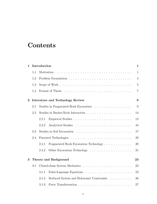
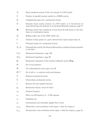
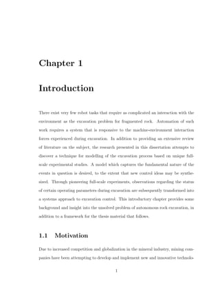
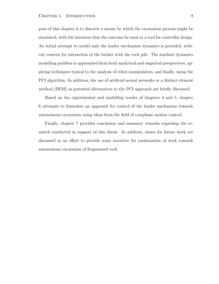
PSfrag replacements boom
bucket
vehicle body
lift cylinder(s)
dump cylinder
Figure 1.1: Schematic drawing of the load-haul-dump (LHD) machine
gies [6]. Among such efforts has been a move towards automated mobile equipment,
including robotic excavation. Although the concept of autonomous excavation has
gained some attention in the last decade, few investigations into the development
of such technologies have been reported for large and non-homogenous excavation
media, such as fragmented rock1
.
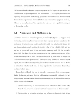
In particular, this thesis focuses on the problem of autonomous excavation using
a load-haul-dump (LHD) underground mining machine. Such LHD machines are
used extensively in underground mining applications to gather and transport ore
from drawpoints to haulage vehicles or underground orepasses. These machines are
easily recognizable by their characteristic geometry. They are a front-end-loader style,
hydraulically actuated, and articulated vehicle. They are typically driven by a diesel
engine or electric motors, while steering is accomplished through application of a
torque at the vertical steering joint that forms the point of articulation. Figure 1.1
presents a schematic drawing that shows the LHD machine geometry used for the
research communicated by this dissertation.
The load-haul-dump cycle is one that is repetitive and hence well suited for au-
1
Herein, the term excavation refers typically to the excavation task carried out in fragmented
rock, as opposed to in other excavation media (e.g. soil or gravel).](https://image.slidesharecdn.com/52609fa3-58a5-4f32-9c85-da30edc9900c-150416073852-conversion-gate02/85/Marshall-MScThesis-2001-18-320.jpg)
![Chapter 1. Introduction 3
tomation. Several parties have attempted to automate the tramming (haul) por-
tion of the load-haul-dump cycle, or have at least proposed solutions to the problem
[17, 35, 57, 74, 99]. To date, most underground navigation systems rely on installed
infrastructure for guidance, although laser and/or camera guided systems are not
far from becoming feasible and economical. Obviously, the problem of autonomously
dumping the bucket load is one that is relatively simple in comparison to autonomous
navigation and bucket loading. Subsequently, the problem of autonomous navigation
is thought to be less complex than that of autonomous loading, for reasons that will
become evident in the following chapters.
The environments in which LHD machines are required to operate tend to be
particularly hazardous in that the loading of ore occurs at underground drawpoints.
These drawpoints often pose the dangers of falling or shifting broken rock during
loading. In order to increase safety during such operations, remote control and tele-
operation technologies have already been developed for LHD operators [48]. The
obvious next step is development of a reliable system for autonomous loading of
fragmented rock.
In addition to increased safety, automation of the loading task has the potential
to provide enhanced productivity, through improved machine utilization and superior
machine performance. Unlike a human operator, an automated machine could remain
steadily productive, irrespective of environmental conditions or prolonged work hours.
In addition, an automated loader might generate more accurate loading, making up
for shortcomings in operator skill. Finally, operator abuse and machine wear would
most likely be diminished through automation, possibly resulting in better machine
reliability and reduced maintenance costs.
As will be seen in chapter 2, despite the fact that a significant amount of pre-
vious work, both theoretical and experimental, has been conducted to address the
autonomous excavation problem, widespread adoption of automated loading has yet](https://image.slidesharecdn.com/52609fa3-58a5-4f32-9c85-da30edc9900c-150416073852-conversion-gate02/85/Marshall-MScThesis-2001-19-320.jpg)
![Chapter 1. Introduction 5
and hardness), the rock pile geometry, and the distribution of particle sizes and
shapes. Indeed, it would be very difficult to predetermine the exact nature of future
bucket-rock interactions prior to the excavation operation.
As will be discussed in chapter 2, others have formulated the autonomous exca-
vation problem in its broadest meaning, incorporating the need for overall planning
of the excavation goal. For example, a possible generalized excavation goal might be:
“Remove a pile and clean the site in an area of D × E m2
centering at (Xm, Ym) in
the coordinate system P” [91, page 3]. However, in this dissertation, consideration
is not given to the problem in this general sense. Instead, focus is devoted to the
question of how to compute the necessary actuator control inputs during the loading
operation, based on sensor feedback and some understanding of the involved pro-
cesses, so that the excavator bucket might be filled completely and reliably at each
loading iteration. In fact, the problem formulation is narrowed further in that only
the lift and dump cylinders are considered as controllable actuators. For the purposes
of this dissertation, an assumption was made that any tractive effort supplied by the
vehicle is generally constant throughout the loading operation, and that control of the
tractive effort would not provide any significant contribution towards an autonomous
excavation system (i.e. effective filling of the bucket relies primarily on the appropri-
ate selection of lift and dump cylinder motions). This assumption is reviewed again
in chapter 7. The scope of this dissertation, in the problem context given above, is
outlined in the section that follows immediately.
1.3 Scope of Work
As will be seen in chapter 2, some previous researchers have considered the problem of
capturing the essential aspects of the excavation process for the purposes of simulation
and controller development to be extremely difficult, if not impossible. Furthermore,](https://image.slidesharecdn.com/52609fa3-58a5-4f32-9c85-da30edc9900c-150416073852-conversion-gate02/85/Marshall-MScThesis-2001-21-320.jpg)
![Chapter 2. Literature and Technology Review 10
[33] presented an analytical study of the loader mechanism geometry and the required
hydraulic cylinder forces through treatment of the mechanism as a robot manipulator.
In [27], Hemami acknowledged that the trajectory control of standard industrial
robots (e.g. welding or cutting robots) is different than the control required for loading
of an LHD bucket. It was suggested that the trajectory a loader bucket should follow
through the rock pile not have priority in the control scheme, since the objective is
to effectively fill the bucket, not to follow a strictly specified path. Some conceptual
discussion was also provided on the topic of motion control. The forces acting on the
bucket were described as potentially stochastic in nature, and the need for trajectory
alteration in the event of detected prematurely high loads on the bucket was stated.
Hemami divided the possible bucket-rock interaction forces into five components:
f1, the weight of the loaded material and that above the bucket; f2, the force of
compacting the material by the bucket; f3, the sum of frictional forces acting between
the bucket and the excavation media; f4, the digging resistance of the excavation
media, and; f5, the necessary force to move the material in and above the bucket.
Means for analytically determining, or at least approximating, some of these dy-
namic forces were subsequently presented in [28, 30, 34]. Along with a relatively
extensive list of suggested future work, Hemami put forth the following as reasons for
the complexity of the excavation problem: (i) the shape, size, geometry and composi-
tion of the cutting device may vary from machine to machine; (ii) adding teeth to the
cutting edge changes the scenario, and; (iii) material properties are determined by
many factors, including hardness, cohesion, uniformity, water content, temperature,
size, and compactness.
A method for determining an appropriate bucket trajectory was presented by
Hemami in [29]. The proposed trajectory generation technique employed the idea
that resistance to compaction described by the force f2 may be set to zero, so as
to minimize the expenditure of energy. However, a method for tailoring the derived](https://image.slidesharecdn.com/52609fa3-58a5-4f32-9c85-da30edc9900c-150416073852-conversion-gate02/85/Marshall-MScThesis-2001-26-320.jpg)
![Chapter 2. Literature and Technology Review 11
loading trajectory was not explained in any detail, and its potential effectiveness at
completely filling the bucket was not determined.
In [31], Hemami essentially repeated the works described above. Nevertheless,
there were some additions that are worth noting. A mathematical model for the
variation of f1 was produced using knowledge about the geometry developed during
the loading operation. Hemami also concluded that an analysis of the force f4 should
be done experimentally.
Finally, in [32], Hemami provided a lengthy discussion of the fundamental analyses
required for the design of an automated excavation machine. One interesting inclusion
in this work was the consideration of a mass-spring-damper model for the excavation
machine, as well as the excavation media (such as is common in compliant motion
analysis). However, it was suggested that this type of model cannot be used in
practice, since there is insufficient understanding of the mass, spring, and damper
coefficients. In addition, the problem of choosing an entity to be exploited as error,
to be measured and used for feedback in a control scheme, was considered. On this,
Hemami stated:
Having taken a look at how an excavating machine is manually operated
reveals that the motion of such a machine is continuously corrected and
readjusted by the operator. This adjustment is based on the performance
of the machine in accomplishing its task. . . and not the motion itself. The
same procedure must be automatically followed in an automated machine
[32, page 178].
It was concluded that trajectory control cannot be entirely based on position or
velocity errors, nor on a vision system that monitors the progress of the excavation
process. A dual-level control was suggested, where a nominal trajectory is followed
and modified through higher-level force measurements.
It should be noted that, of the works reviewed to this point in the thesis, none
of the given results or ideas were reported as having been verified by experimental
means; not in full-scale, nor in laboratory-scale excavation experiments.](https://image.slidesharecdn.com/52609fa3-58a5-4f32-9c85-da30edc9900c-150416073852-conversion-gate02/85/Marshall-MScThesis-2001-27-320.jpg)
![Chapter 2. Literature and Technology Review 12
Other authors have approached the problem of autonomous rock excavation from
a perspective similar to Hemami’s. Generalized machine dynamics were set up by
Sarata et al. [86], although not actually computed. As will be seen in chapter 5,
computation of these dynamics is in fact not an entirely trivial matter. Under a
pioneering Russian project, Mikhirev formulated a set of ideas relating to force, mo-
tion, and trajectory control for various loader mechanism styles [61, 62]. Mikhirev’s
analysis was based on a technique using work functions to find an efficient bucket
trajectory that would minimize the work for scooping rock masses, with complete
filling of the bucket. Additional constraints were determined by the bucket capacity,
the natural slope angle, and the pile height. The resistive force modelling portion
of this research is discussed further in subsection 2.2.1. However, as a result of rock
pile resistance analysis, Mikhirev advocated that measurement of the resistive forces
could be used as a signal for automatic activation of the mechanism for bucket rota-
tion in the vertical plane (which, in the case of an LHD machine, would correspond
to motions of the dump cylinder). Since reactive forces were thought to decrease as
the bucket moved along a continuous curvilinear path towards the pile surface, it was
proposed that a force threshold be used to alter the bucket trajectory, resulting in a
stepped path (i.e. zig-zag shape) along some nominal trajectory.
In other literature, machine vision has been put forward as a means for au-
tonomous loading of mining machines. In the research of Ji and Sanford [37], a
laboratory-scale excavation system was developed that utilized a video camera for
environment sensing. Digitized images were then interpreted to develop control and
navigation signals. More recent work, using machine vision, has been performed by
Petty et al. [73]. Once again, a scale model was developed. However, in this case, the
model was constructed to mimic the motions of an LHD vehicle as closely as possible.
A loading strategy was formulated such that the bucket followed one of a range of
trajectories developed for various rock pile conditions. In the case of oversize or other](https://image.slidesharecdn.com/52609fa3-58a5-4f32-9c85-da30edc9900c-150416073852-conversion-gate02/85/Marshall-MScThesis-2001-28-320.jpg)
![Chapter 2. Literature and Technology Review 13
problems, it was suggested that a simple algorithm be used to briefly alter the bucket
path. The proposed algorithm included a means of detecting instability in the rock
pile as well as choosing the location where scooping should take place at the next
iteration.
Similar, though perhaps more rigorous, research techniques were employed by
a group at Tohoku University in Japan [104]. A CCD camera vision system was
used to obtain images of the rock pile, from which the excavation task was planned
based on an estimated contour of the rock pile. Experiments were performed using
a scale model excavator, similar in configuration to an LHD machine. The authors
suggested that such a camera based system would be advantageous in its capability
for recognizing changes in rock pile shape at each iteration towards the excavation
goal. Although the results were promising, it was conceded that illumination became
an important factor for success, a problem that would likely be compounded in an
underground mining situation. This research is of the type described in section 1.2,
which falls beyond the scope of this dissertation.
Researchers at the University of Arizona have proposed an autonomous rock ex-
cavation system for front-end-loader type machines that uses bucket force/torque
feedback, fuzzy logic, and neural networks for control [51, 52, 90]. Lever et al. [51]
justified their approach by stating that a mathematical model for the bucket-rock
interaction would be too complex and computationally expensive. Instead, a set of
basic bucket action sequences, typically used by human operators, was compiled for
use by the controller. A method using finite-state machines (FSMs) was described.
The FSMs were used to define all feasible action sequences required to accomplish
the task, and were derived from “expert excavator operators and detailed analyses of
the excavation process” [52, page 137]. Neural networks were used in the FSMs to
determine what state to enter following an action or behaviour. A reactive control
approach, using fuzzy behaviours, was utilized to compare and act on force/torque](https://image.slidesharecdn.com/52609fa3-58a5-4f32-9c85-da30edc9900c-150416073852-conversion-gate02/85/Marshall-MScThesis-2001-29-320.jpg)
![Chapter 2. Literature and Technology Review 14
data in order to asses the excavation situation and determine the appropriate con-
trol output. Some experimental results using a PUMA 560 robotic arm were also
presented. This work is fully disclosed in a recent book by the authors [91].
2.2 Studies in Bucket-Rock Interaction
What makes the excavation of coarse, fragmented rock significantly different than that
of ideal, homogeneous materials is that there is not one defined shear plane. In order to
force an excavation tool through fragmented rock it is necessary to not only overcome
the particle to particle frictional resistance, but also to make the particles move up
and over one another [22]. In justifying their behaviour-based control approach to the
problem at hand, Lever et al. [51] argued the difficulties of mathematically modelling
the excavation tool-media interaction.
It is impossible to generate a rigorous mathematical model to describe the
unstructured environments common in mining operations. The conven-
tional proportional-integral-derivative (PID) or even modern stochastic
controllers that read exact sensor values, apply a mathematical model,
and generate precise output from the mathematical algorithm are im-
practical for use here [51, page 18].
However, it is the candidate’s view that, although the problem of rock pile interaction
modelling may be very difficult to quantify, it should not be considered as a decidedly
impossible task, as suggested in the above quotation. Moreover, such difficulties
should not preclude the use of an approach to the excavation problem based on ideas
from systems and control theory. As will be shown, some headway has been made in
this avenue by other researchers in the field.
2.2.1 Empirical Studies
Some interesting empirical work was done by Forsman and Pan [22] regarding the
shear properties of fragmented rock. Loose material, such as broken rock, will not](https://image.slidesharecdn.com/52609fa3-58a5-4f32-9c85-da30edc9900c-150416073852-conversion-gate02/85/Marshall-MScThesis-2001-30-320.jpg)
![Chapter 2. Literature and Technology Review 15
move (i.e. fail) until the applied force reaches a yield level, called the shear strength for
granular media. The shear strength of fragmented rock is hence an important property
in the context of material loading. Forsman and Pan suggested an improvement over
Coulomb’s equation, commonly used for modelling fine grained materials, in the form
of a mathematical expression, derived empirically, for the shear strength of large
grained loose material. It is interesting to note that the material porosity was implied
to be related to the size distribution of a fragmented rock pile, as well as the degree
of interlocking between particles. In addition, Forsman and Pan related the material
porosity to fluctuations of the measured normal force in their experimental results.
Analysis of the resistance of fragmented rock to scooping by a bucket was reported
in some Russian literature [21, 61]. With regards to the work by Fabrichnyi and
Kolokolov [21], a means for calculation of the scooping resistance to blasted rock was
given, based on knowledge of the rock pile’s changing shear angle.
It is known that in general the scooping force is governed by the volume
of the rock to be shifted, which in turn depends on the angle between the
horizontal and the shear surface of the rock. The experimentally recorded
variations in the scooping resistance can only be due to changes in the
inclination of the shear surface, leading to increases or decreases in the
volumes of rock being shifted [21, page 438].
Unfortunately, key references were made by Fabrichnyi and Kolokolov to obscure
experimental work (performed much earlier, circa 1957, and available only in the
Russian language) by an investigator named Rodionov [79].
In related work, Mikhirev [61] reported some potentially applicable results. Al-
though techniques for control and bucket trajectory generation were the focus of this
research, insight into the forces associated with resistance to movement of the bucket
through rock was provided. Mikhirev cited the experimental research of Rodionov,
which apparently established that a compact nucleus is created in the pile in front
of the working edge of the bucket. The characteristics of this compact nucleus were
found to relate most notably to average particle size, bucket shape, and bucket pose.](https://image.slidesharecdn.com/52609fa3-58a5-4f32-9c85-da30edc9900c-150416073852-conversion-gate02/85/Marshall-MScThesis-2001-31-320.jpg)
![Chapter 2. Literature and Technology Review 16
2.2.2 Analytical Studies
Hemami et al. [34] acknowledged that the forces involved in excavating fragmented
rock are functions of a large number of parameters, which makes the study of such
forces particularly difficult. In this work, Hemami et al. categorized the various
physical factors that contribute to the complexity of the problem. Major categories
included the operation to be performed, the form of the excavation tool to be used,
the material properties, and other machine or application factors. In further studies
of the forces acting on a bucket during a scooping operation, Hemami et al. identified
five force components. The cited article gave references to works where analysis of
these forces had been attempted (see section 2.1). Some simulation results were also
presented. However, it was admitted that random fluctuations of these forces would
likely exist in reality.
Perhaps the most relevant and complete research in bucket-rock interaction mod-
elling is some very recent work completed at Tohoku University, in Japan [102, 105].
In this work, Takahashi et al. essentially proposed a means for calculation of each of
the resistive forces {f1, . . . , f5} described previously by Hemami (again, see section
2.1). For analysis purposes, the loading operation was partitioned into two stages:
(i) a penetration phase, where the bucket is inserted into the rock pile, and; (ii) a
scooping phase, where the bucket tip is lifted and curled to complete the loading task.
Given an assumed bucket trajectory, the resistive forces were computed analytically
using geometric and frictional parameters of the bucket and rock pile. Equivalent
scale model experimental results confirmed the calculated forces to be approximately
valid. Unfortunately, the derived equations failed to capture the inherently stochastic
nature of the loading process.
Analytical research has been completed in the area of numerical modelling of
granular assemblies. Consider the work by Cundall and Strack [14], where a distinct
element method (DEM) was used to numerically model the mechanical behaviour of](https://image.slidesharecdn.com/52609fa3-58a5-4f32-9c85-da30edc9900c-150416073852-conversion-gate02/85/Marshall-MScThesis-2001-32-320.jpg)
![Chapter 2. Literature and Technology Review 17
assemblies of discs (and spheres in three dimensions). “The method is based on the
use of an explicit numerical scheme in which the interaction of the particles is moni-
tored contact by contact and the motion of the particles modelled particle by particle”
[14, page 47]. In recent work by Takahashi [101], the ideas of Cundall and Strack were
applied to simulation of particle behaviour in a virtual rock pile. Excavation of a rock
pile having uniformly sized particles was simulated using a DEM approach and the
bucket-rock interaction forces were computed for a predetermined trajectory. Once
again, equivalent scale model experimental results confirmed the simulated interac-
tion forces to be approximately valid. However, it was also admitted that full-scale
experiments would be required to truly validate the given computational results. This
technique is discussed further in chapter 5.
2.3 Studies in Soil Excavation
What distinguishes the problem of autonomous excavation of fragmented rock from
the research presented in this section is simply the nature of the excavation media.
In general, the work discussed in this section concerns itself with the problem of
soil excavation. Soil, as opposed to fragmented rock, is generally homogeneous in
particle size and typically consists of relatively small particles, such that a bucket
may be passed through it without the need for significant trajectory alteration. Soil
excavation could be appropriately characterized as a cutting exercise, rather than
the task of maneuvering a bucket such that it is properly filled with large and small
fragments alike, since forces at the tool would evolve smoothly instead of abruptly.
Nonetheless, research in this field shares some common attributes with the problem
of rock excavation. Moreover, the lack of commercial technology seems to contrast
the fact that there appears to have been a considerable amount of research completed
in the field of autonomous soil excavation. In this section, only a selection of the](https://image.slidesharecdn.com/52609fa3-58a5-4f32-9c85-da30edc9900c-150416073852-conversion-gate02/85/Marshall-MScThesis-2001-33-320.jpg)
![Chapter 2. Literature and Technology Review 18
relevant literature is presented.
The problem of autonomous excavation in soil was approached from a motion and
path control perspective by Bernold [9]. Bernold advocated the use of impedance
control, utilizing force and position feedback. In the case of robotic excavation, the
robot was considered as an impedance, translating motion into force, and the soil as
an admittance, reacting with a change in position or motion. A mass-spring-damper
model for the tool-soil interaction was presented. An attempt was made to determine
an optimal path for excavation. With regards to this effort, Bernold concluded:
In summary, the selection of an optimal path, resulting in lowest energy
consumption per excavated volume, is a nontrivial problem which hinges
mostly on the proper characterization of the soil-tool interaction and the
soil itself. Although static soil experiments can provide the cohesion fac-
tor, the complexity of the remaining coefficients for cutting-moment cal-
culation make a static approach to the problem impossible [9, page 9].
To this end, a method of trajectory selection using pattern recognition was suggested.
Experimental work was performed using a scale modelled backhoe style excavator (a
modified RM-501 micro-robot). Force and position data were collected to create char-
acteristic patterns for various soil conditions. Results were used only to show that
it may be conceivable that soil characteristics could be established while excavating,
leading to the possibility for trajectory planning and control for autonomous exca-
vation. A similar approach, using impedance control for backhoe excavation control,
was also proposed by Ha et al. [26]. In this recent work, a sliding-mode controller for
impedance control was developed. Having developed kinematic and dynamic models
for the excavator, the control scheme was subsequently implemented, with apparently
promising results, on a retrofitted Komatsu PCI05-7 mini-excavator.
V¨ah¨a and Skibniewski [106] presented a method of cognitive force control for an
excavator. A dynamic model was developed for the excavator and used in conjunction
with a model for the soil (referred to as the regolith), which was based on the break-
down of resistive forces into a resistance from cutting, frictional resistance, and the](https://image.slidesharecdn.com/52609fa3-58a5-4f32-9c85-da30edc9900c-150416073852-conversion-gate02/85/Marshall-MScThesis-2001-34-320.jpg)
![Chapter 2. Literature and Technology Review 19
resistance of the material in the bucket. Further details of the backhoe style excavator
dynamic model were derived later in a publication by Koivo et al. [41]. Simulation
results compared the preplanned bucket trajectory with its actual trajectory, which
was adjusted when hydraulic ram forces exceeded preset limits. In a technique pro-
posed by Bullock and Oppenheim [10], strain gauges were used during a laboratory
study to measure the resistive forces encountered by the excavator bucket. A super-
visory control scheme, where force feedback data are processed at a higher level to
produce low level trajectory changes, was considered as an online tactical planner for
excavation.
There exists an apparently ongoing project at the University of Sydney, Australia
that aspires to develop a system for autonomous excavation [50]. Although it was
stated that the ultimate objective of the project is to demonstrate fully autonomous
excavation for a variety of tasks, including excavation not only in soil but also in
fragmented rock, the described experimental hardware consisted of a backhoe style
mini-excavator. It was implied that future experiments and analyses were to be
carried out in soil type media.
Researchers at Carnegie Mellon University [95] proposed a technique for robotic
excavators to predict resistive forces during excavation using computer learning meth-
ods. Included in the presented work is a development of the mechanics of excavation,
resulting in the formation of what is known as the fundamental equation of earthmov-
ing (FEE) for a flat blade moving through soil. The assumptions required to validate
the FEE were used by the authors to demonstrate its impracticality in the context of
excavation.
More recent work at Carnegie Mellon University [7, 81, 100] has resulted in a
patented system for robotic excavation and autonomous truck loading. In summary,
the system described utilized two scanning laser range-finders to recognize and localize
the truck, measure the soil face, and detect obstacles. Onboard software was used](https://image.slidesharecdn.com/52609fa3-58a5-4f32-9c85-da30edc9900c-150416073852-conversion-gate02/85/Marshall-MScThesis-2001-35-320.jpg)
![Chapter 2. Literature and Technology Review 20
to make decisions regarding digging and dumping operations. Actual digging was
described as executed by a force based closed loop control scheme, after previous
research in excavation planning by one of the authors. Dumping and truck detection
routines were also included as part of the project.
2.4 Patented Technologies
In this section, a selection of patented technology is presented in order to provide
an understanding of the work that has been considered commercially feasible. The
majority of existing patents relate to the automation of soil excavation tasks, generally
using backhoe style excavators [7, 76, 81, 92, 93, 94]. However, there does exist
recent work relevant to autonomous excavation of fragmented rock, using LHD-style
machinery, as in an underground mining application. It is these patents that are
discussed in the subsections that follow.
2.4.1 Fragmented Rock Excavation Technology
A review of the current patents relevant to the problem of autonomous bucket loading
revealed two significant contributions. The most recent, by Dasys et al. [15], as part
of a group representing the international mining and metals company Noranda, Inc.,
revealed a patented system for automated bucket loading of a front shovel loader
(i.e. an LHD) that uses “sensor feedback provided by pressure and extension sensors
on hydraulic cylinder(s) to control the trajectory of the bucket to be loaded by a
computer algorithm” [15]. The described invention does not rely on a model of the
rock pile, nor is there any computational attempt to determine an optimal bucket
trajectory prior to the scooping operation. Instead, the system reacts, using a decision
tree to select actuator commands, only to excessive forces sensed in the actuating
cylinders. If excessive forces are encountered, the bucket is tilted so as to attempt to](https://image.slidesharecdn.com/52609fa3-58a5-4f32-9c85-da30edc9900c-150416073852-conversion-gate02/85/Marshall-MScThesis-2001-36-320.jpg)
![Chapter 2. Literature and Technology Review 21
dislodge the rock or other hinderance causing the disproportionate force.
The computer. . . has a [hybrid] controller which controls the hydraulic
valve that supplies hydraulic fluid into both ends of the [bucket dump]
cylinder. . . and if too much force is exerted on the bucket by the rock
pile, the command for hydraulic fluid intake will be reversed and the fluid
will be injected into the opposite side of the piston. . . so as to reverse
the action of the shaft. . . until the force drops to a predetermined level.
Then, the oil intake will be reversed again and the tilting action of the
bucket will be resumed until the bucket. . . is filled and is in the rolled back
position. . . [15].
Furthermore, Dasys et al. claimed a 9% improvement in loading capacity, com-
paring their invention with human operation in field trials. A paper related to the
work by Dasys et al. was put forward at the 5th International Symposium on Mine
Mechanization and Automation by representatives from STAS Ltd. [49], partners in
the Noranda, Inc. project. Unfortunately, no technical details were given in the paper.
However, the user-level features of the product, entitled SIAMload, were presented. It
is worth noting that SIAMload required that an operator choose one of three loading
modes, depending on the human perceived loading conditions.
2.4.2 Other Excavation Technology
A second relevant patent in autonomous excavation was filed by Rocke, a represen-
tative of Caterpillar, Inc. [77]. In Rocke’s invention, a control system for automatic
loading of a wheel loader (similar in mechanical design to an LHD machine), which is
particularly suited to soil excavation, is disclosed. Although references were made to
a number of previous patents by the inventor (all of which applied to backhoe style
soil excavation), in the current patent, an algorithm that appears very similar to the
one that was patented three years later by Dasys et al. (discussed in subsection 2.4.1
above) is given.
As described,the logic means varies the dump cylinder command signal
between a predetermined minimum and maximum value to maintain the](https://image.slidesharecdn.com/52609fa3-58a5-4f32-9c85-da30edc9900c-150416073852-conversion-gate02/85/Marshall-MScThesis-2001-37-320.jpg)
![Chapter 2. Literature and Technology Review 22
lift and dump cylinder forces at an effective force range. Accordingly
the positions and forces of the lift and dump cylinders are monitored to
control the command signals at the desired magnitudes. For example, if
the lift or dump cylinder forces fall below the lower predetermined values,
the extension of the dump cylinder is halted to prevent the bucket from
“breaking-out” of the pile too quickly. Alternatively, if the lift or dump
cylinder force exceeds the upper predetermined value, the extension of the
dump cylinder is accelerated to prevent the bucket from penetrating too
deep in the pile [77].
Furthermore, it should be noted that control of the vehicle tractive effort was not
included in the control strategy as stated, and that the machine was preferably di-
rected to the pile of material at full engine throttle. On the matter of adaptability
of the system to varying material conditions, the reader was referred to [78], another
patent by the inventor, in which a system for selecting one of a plurality of control
curves based on a material condition setting, is disclosed.
In essence, the common theme in these two patents [15, 77] is a cylinder motion
control scheme based on some interpretation of the changing pressures in the hydraulic
cylinders as an indication of the state of the bucket-rock interaction.](https://image.slidesharecdn.com/52609fa3-58a5-4f32-9c85-da30edc9900c-150416073852-conversion-gate02/85/Marshall-MScThesis-2001-38-320.jpg)
![Chapter 3
Theory and Background
In this chapter, background reviews of the relevant theory in the formulation of equa-
tions of motion for closed-chain kinematic mechanisms and techniques for nonlinear
system modelling and identification are provided. The purpose here is to provide a
concise theoretical background for the thesis material that follows.
3.1 Closed-chain System Mechanics
In chapter 5, analytical equations of motion for the Tamrock EJC 9t LHD loader
mechanism are formulated through treatment of the mechanism as a robot manip-
ulator with closed kinematic chains. Herein, the term closed-chain system refers to
the class of mechanical systems whose links are not only connected in series, but in
parallel, forming one or more closed-link loops. As opposed to an open-chain system
(e.g. a serial robot), typically not all joints of a closed-chain mechanism are actuated.
Such closed-chain mechanisms have the potential to offer some mechanical advantages
over open-chain mechanisms, perhaps most notably, a greater rigidity to weight ratio.
The dynamics of open-chain mechanical systems have been extensively studied
in the literature, and there exist well established techniques for the formulation of
equations of motion for such mechanisms [53, 98, 107]. In essence, in the absence of
23](https://image.slidesharecdn.com/52609fa3-58a5-4f32-9c85-da30edc9900c-150416073852-conversion-gate02/85/Marshall-MScThesis-2001-39-320.jpg)
![Chapter 3. Theory and Background 24
friction and interaction with the environment, equations of motion for an open-chain
system may be computed using a standard Newton-Euler or Lagrangian approach.
Although there exists a multitude of literature on the subject, due to the complex-
ity of the kinematic and dynamic analyses, development of a clear-cut technique for
the derivation of equations of motion for closed-chain mechanisms remains a topic of
research. Ghorbel et al. [25] attempted to categorize the literature on the derivation
of dynamic equations of motion for closed-chain mechanisms into three classes: (i)
those techniques derived for a particular type of closed-chain structure; (ii) those tech-
niques derived for general closed-chain structures, but most suited for simulation and
not model-based controller design, and; (iii) those techniques for which the resulting
equations of motion have the same form as those for open-chain structures. Among
the reviewed literature [25, 55, 56, 65, 66], the formulation of Murray and Lovell [65],
which falls into category (iii) of Ghorbel et al., was selected by the candidate as a
framework for use in this dissertation.
The approach proposed by Murray and Lovell [65] involves a relatively straight-
forward procedure for implementation. The method is founded upon d’Alembert’s
Principle1
and is based around a transformation from the dynamics of open-chain
mechanisms to closed-chain dynamics through the inclusion of holonomic loop con-
straints.
3.1.1 Euler-Lagrange Equations
Computation of the dynamics for closed-chain mechanisms, as described above, is
based on a transformation from open-chain systems using holonomic constraints.
Later in this dissertation, the Euler-Lagrange equations are used in the derivation
of equations of motion for an open-chain system (as will be seen in the next sub-
1
In brief, d’Alembert’s Principle, considered perhaps the most all-inclusive principle in the entire
field of classical mechanics, states that a system of particles moves in such a way that the total
virtual work
p
i=1(f − mi ¨xi) · δxi = 0 [97].](https://image.slidesharecdn.com/52609fa3-58a5-4f32-9c85-da30edc9900c-150416073852-conversion-gate02/85/Marshall-MScThesis-2001-40-320.jpg)
![Chapter 3. Theory and Background 25
section). This section serves to provide an applied introduction to the subject of
Lagrangian mechanics as it is relevant to the problem at hand. However, the topic
is extensive, and the reader is referred to [53, 98, 107] for further details and formal
derivations.
Definition 3.1.1 A configuration space Q represents the set of possible configurations
of a mechanical system.
Definition 3.1.2 The set of generalized coordinates {q1, . . . , qn} are independent,
and sufficient to describe the pose of all particles in a mechanical system with n
degrees of freedom.
Let Q be a configuration space for a mechanical system, so that the vector of gener-
alized coordinates q ∈ Q. The Euler-Lagrange equations are then given by
d
dt
∂L
∂ ˙qi
−
∂L
∂qi
= τi (3.1)
where {q1, . . . , qn} are the coordinates of the system, {τ1, . . . , τn} are the applied
forces2
corresponding to independent variations of qi, and L = K−V is the Lagrangian
function describing the given mechanical system, defined as the difference between
the total kinetic energy K of the system and the total potential energy V of the
system. If the Euler-Lagrange equations of (3.1) are specialized to a case when the
kinetic energy is a quadratic function of the vector ˙q that has the form
K =
1
2
n
i,j=1
dij(q) ˙qi ˙qj (3.2)
and the potential energy V = V (q) is independent of ˙q, then the Euler-Lagrange
equations may be written as
n
j=1
dkj(q)¨qj +
n
i=1
cijk(q) ˙qi ˙qj + φk(q) = τk (3.3)
2
Herein, the term force is used to mean force and/or torque.](https://image.slidesharecdn.com/52609fa3-58a5-4f32-9c85-da30edc9900c-150416073852-conversion-gate02/85/Marshall-MScThesis-2001-41-320.jpg)
![Chapter 3. Theory and Background 26
for k = 1, . . . , n, and where the terms cijk are known as Christoffel symbols [53, 98].
Equation (3.3) may be written in matrix form, such that
D(q)¨q + C(q, ˙q) ˙q + g(q) = τ (3.4)
where the k, j-th element of the matrix C(q, ˙q) is defined as
ckj =
n
i=1
cijk(q) ˙qi
=
n
i=1
1
2
∂dkj
∂qi
+
∂dki
∂qj
−
∂dij
∂qk
˙qi (3.5)
and the vector of gravitational potential terms g(q) has the elements
φk =
∂V (q)
∂qk
. (3.6)
3.1.2 Reduced System and Holonomic Constraints
The notion of a reduced system is required as the first step in developing the closed-
chain mechanism dynamics.
Definition 3.1.3 A reduced system Σ is an open-chain system obtained by hypo-
thetically removing physical constraints from a closed-chain system ˜Σ until no closed
kinematic chains exist.
Therefore, formation of the reduced system involves the construction of an open-chain
mechanism, obtained by treating the closed-chain mechanism as if it were cut upon at
selected joints such that no closed-loops remain. It is often convenient to strategically
choose the constraints to be broken so that the resulting reduced system resembles a
serial robot, for which there exist well known techniques for analysis.
Now, if ˜Q = m
is a configuration space for a closed-chain system ˜Σ with the
actuated joints3
as generalized coordinates ˜q ∈ ˜Q, then let Q = n
be a configuration
3
For this research, to match the experimental trials of chapter 4, the actuated and measured
joints are collocated, i.e. the coordinates of the closed-chain system are the measured joint variables.](https://image.slidesharecdn.com/52609fa3-58a5-4f32-9c85-da30edc9900c-150416073852-conversion-gate02/85/Marshall-MScThesis-2001-42-320.jpg)
![Chapter 3. Theory and Background 27
space for the corresponding reduced system Σ, having the generalized coordinates
q ∈ Q. To derive the closed-chain mechanism dynamics from the reduced system
dynamics, the holonomic4
loop closure constraints are required, so that
q = f(˜q) . (3.7)
The velocity loop closure constraint matrix G, with respect to the actuated joints, is
also needed, such that
˙q = G ˙˜q (3.8)
where the Jacobian matrix G ∈ m×n
. Finally, the acceleration loop closure con-
straint, stemming from the time derivative of equation (3.8), is required and may be
found by the chain rule, giving
¨q = G¨˜q + ˙G ˙˜q . (3.9)
3.1.3 Force Transformation
Consider the set of generalized actuating forces {τ1, . . . , τm} for the open-chain system
Σ and similarly, {˜τ1, . . . , ˜τn} for the closed-chain system ˜Σ.
Proposition 3.1.1 Let G be the Jacobian matrix defining the relation δq = Gδ ˜q.
The vector of generalized forces ˜τ for ˜Σ may be computed from the vector of generalized
forces τ for Σ by the transformation
˜τ = GT
τ . (3.10)
The proof of proposition 3.1.1 lies in the application of d’Alembert’s Principle. A full
proof is given by Nakamura and Ghodoussi in [66]. However, since Σ and ˜Σ represent
the same mechanical system only under different constraints, consider that the virtual
4
A constraint on the coordinates {q1, . . . , qn} is called holonomic if the constraint condition can
be expressed as an equation φ(q1, . . . , qn, t) = 0, otherwise it is called non-holonomic [97].](https://image.slidesharecdn.com/52609fa3-58a5-4f32-9c85-da30edc9900c-150416073852-conversion-gate02/85/Marshall-MScThesis-2001-43-320.jpg)
![Chapter 3. Theory and Background 28
work done by the generalized forces of Σ must equal the virtual work done by the
generalized forces of ˜Σ if the two systems experience the same applied forces. Hence,
δ ˜qT
˜τ = δqT
τ (3.11)
where δ ˜q and δq represent the same virtual displacement of the mechanical system.
Substituting equation (3.8) into equation (3.11) yields
δ ˜qT
˜τ = δ ˜qT
GT
τ . (3.12)
Equation (3.10) follows directly from equation (3.12).
3.1.4 Closed-chain Equations
Given the reduced system dynamics and the holonomic loop closure constraints, the
closed-chain mechanism dynamics may be computed. Through application of the
generalized actuating force transformation of equation (3.10), which relates the closed-
chain mechanism dynamics to the reduced system dynamic model
GT
[D(q)¨q + C(q, ˙q) ˙q + g(q)] = ˜τ . (3.13)
To account for the restriction that the reduced system variables {q, ˙q, ¨q} must be
realizable by the closed-chain mechanism, the holonomic loop closure constraints are
incorporated into equation (3.13) to give
GT
D(f(˜q)) G¨˜q + ˙G ˙˜q + C(f(˜q), G ˙˜q)G ˙˜q + g(f(˜q)) = ˜τ . (3.14)
Equation (3.14) may be rewritten as
˜D(˜q)¨˜q + ˜C(˜q, ˙˜q) ˙˜q + ˜g(˜q) = ˜τ (3.15)
where the inertial coefficient matrix and vectors representing centripetal, Coriolis,
gravitational, and externally applied forces are defined respectively by
˜D(˜q) = GT
D(f(˜q))G (3.16)
˜C(˜q, ˙˜q) = GT
D(f(˜q)) ˙G + GT
C(f(˜q), G ˙˜q)G (3.17)
˜g(˜q) = GT
g(f(˜q)) . (3.18)](https://image.slidesharecdn.com/52609fa3-58a5-4f32-9c85-da30edc9900c-150416073852-conversion-gate02/85/Marshall-MScThesis-2001-44-320.jpg)
![Chapter 3. Theory and Background 30
and correlation methods [96]. Where controller design is concerned, identification of
a linear model is often desirable over one that is nonlinear in that there exist well
known and proven procedures for controller design. However, in the use of a linear
model, one must understand the degree of validity of the linearization assumption.
For the nonlinear case, most system identification approaches involve error minimiza-
tion (e.g. least-squares, maximum likelihood, minimum variance, and artificial neural
networks) to fit acquired data in an attempt at a general model [60, 80, 96].
In this section, the nonlinear system identification technique known as paral-
lel cascade identification (PCI) is introduced. As a prelude to this introduction, a
descriptive review of some nonlinear system theory is provided as it is relevant to
understanding the origins of the PCI algorithm.
3.2.1 Volterra and Wiener Theories
In the context of applied mathematics and engineering, the Volterra and Wiener
theories for nonlinear systems are explicit models ideally suited to representation of
so-called black box type nonlinear systems, where the relationship between the input
and the output of a system is not easily derivable through the development of a
set of equations or other analytical techniques. It can be shown that the Volterra
functional series5
may be used to represent a time invariant nonlinear system. The
continuous-time, infinite-order Volterra series has the functional form
y(t) =
∞
−∞
k1(τ1)x(t − τ1)dτ1
+
∞
−∞
∞
−∞
k2(τ1, τ2)x(t − τ1)x(t − τ2)dτ1dτ2
+ · · · +
∞
−∞
· · ·
∞
−∞
kn(τ1, τ2, . . . , τn)x(t − τ1)x(t − τ2) · · ·
x(t − τn)dτ1dτ2 · · · dτn + · · · (3.23)
5
The Volterra functional series was named after the mathematician Vito Volterra, who first
studied this functional form during the seventeenth century. However, the first application of the
Volterra series to the study of nonlinear systems was by Norbert Wiener in the early 1940s [82, 88].](https://image.slidesharecdn.com/52609fa3-58a5-4f32-9c85-da30edc9900c-150416073852-conversion-gate02/85/Marshall-MScThesis-2001-46-320.jpg)
![Chapter 3. Theory and Background 31
where n = 1, 2, . . ., x(t) is the nonlinear system input, y(t) is the corresponding
output, and kn(τ1, . . . , τn) = 0 for any τj < 0, with j = 1, 2, . . . , n. The functions
kn(τ1, . . . , τn) are known as the Volterra kernels of the system. However, there are
certain inherent difficulties with the application of the Volterra series to physical
problems, some of which include difficulty in the measurement of Volterra kernels,
as well as issues concerning convergence of the Volterra series [88]. It was Wiener
who circumvented these problems by forming a set of orthogonal functions from the
Volterra functionals, which he called G-functionals due to their special orthogonal
property when the input is from a Gaussian process. For example, if the set of real
functions wn(t) for n = 1, 2, . . . is an orthogonal set of functions over the interval
a < t < b, then the orthogonality condition is given by the equation
b
a
wm(t)wn(t)dt =
λn for m = n
0 for m = n
(3.24)
where each λn is positive since it is equal to the area under the curve w2
n(t). In
effect, the Volterra and Wiener theories together have provided a basis for significant
advances in nonlinear system theory.
Korenberg [47, 44] utilized the Volterra and Wiener theories, along with the results
of other related works, to show that any discrete-time, finite-memory, causal, nonlin-
ear system having a finite-order Volterra series representation can be represented by a
finite number of parallel cascades consisting of alternating dynamic linear and static
nonlinear elements. The stated causal requirement necessitates that the system be
non-anticipatory, or in other words, that the output at time ti not depend on values
of the input at times tj, where j > i. The discrete-time, finite-order Volterra series
that is assumed capable of approximating the nonlinear system has the form
y(n) = k0 +
M
m=1
R
r1=0
· · ·
R
rm=0
km(r1, . . . , rm)x(n − r1) · · · x(n − rm)
(3.25)
for n = 1, 2, . . ., where x(n) and y(n) are the system input and output respectively,
M is the order of the series, and (R + 1) is the memory length.](https://image.slidesharecdn.com/52609fa3-58a5-4f32-9c85-da30edc9900c-150416073852-conversion-gate02/85/Marshall-MScThesis-2001-47-320.jpg)
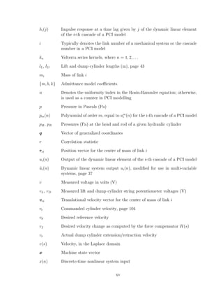
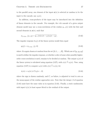
![Chapter 3. Theory and Background 32
x(n)
- L1
-
u1(n)
N1
z1(n)
? -
y(n)
- L2
-
u2(n)
N2
-
z2(n)
- LI
-
uI(n)
NI
zI(n)
6
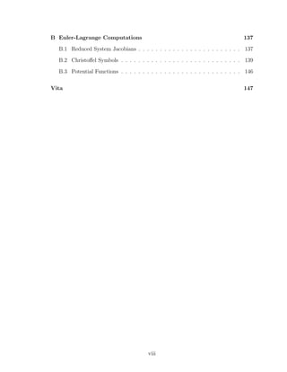
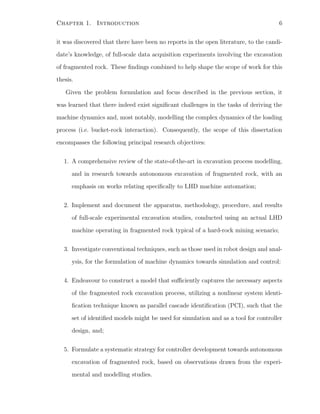
Figure 3.1: Parallel LN cascade schematic model
3.2.2 Parallel Cascade Identification
This subsection summarizes the method of parallel cascade identification (PCI), as
it was used in the research described by this dissertation, and as interpreted from
the work of Korenberg [44]. Details regarding implementation of the algorithm are
provided later, upon use in chapter 5.
Description of the Algorithm
PCI utilizes parallel cascades of alternating dynamic6
linear L and static nonlinear
N elements to represent and identify a nonlinear system. Korenberg [44] showed that
the sum of a finite number of parallel LN cascades suffices to represent exactly any
discrete-time, finite-memory, finite-order Volterra series, sometimes referred to as a
Wiener model. A schematic representation of the proposed parallel cascade model
structure is shown in figure 3.1.
For the single-input/single-output (SISO) case, suppose that the nonlinear system
to be identified has input x(n) and output y(n), for n = 0, 1, . . . , T. Assume that
the system output depends on input delays in the integer set {0, 1, . . . , R}, such that
(R + 1) is the memory length, and that the set of inputs to the system are uniformly
6
In the current context, the term dynamic is used to imply that the system possesses memory.](https://image.slidesharecdn.com/52609fa3-58a5-4f32-9c85-da30edc9900c-150416073852-conversion-gate02/85/Marshall-MScThesis-2001-48-320.jpg)
![Chapter 3. Theory and Background 33
bounded in that there exists a number 0 < N < ∞ such that |x(n)| < N for all
n ⊂ [0, T]. PCI attempts to identify one LN cascade at a time, and computes the
succeeding cascade based on the residual of the previous cascades combined. Let yi(n)
be the residue remaining after adding the i-th cascade (i ≥ 1) to the PCI model, with
y0(n) = y(n). If zi(n) is computed as the output of the i-th cascade, as shown in
figure 3.1, then
yi(n) = yi−1(n) − zi(n) (3.26)
where i = 1, 2, . . . , I are the number of cascades in the final PCI model, yet to be
determined.
Let the output of the dynamic linear element in the i-th cascade be given by
Li : ui(n) =
R
j=0
hi(j)x(n − j) (3.27)
Now, the delta response hi(j) of the linear system is chosen using a first- or higher-
order cross-correlation of the input with the residue, computed only over the interval
n = R, (R + 1), . . . , T. For example, by definition
φxyi−1
(j) = yi−1(n)x(n − j) (3.28)
φxxyi−1
(j1, j2) = yi−1(n)x(n − j1)x(n − j2) (3.29)
where φxyi−1
and φxxyi−1
are first- and second-order cross-correlations of the input
with the residue, respectively, and where the over-line denotes the time-average7
on
the interval n = R, (R + 1), . . . , T. Assign hi(j) at random to one of
q1(j) = φxyi−1
(j) (3.30)
q2(j) = φxxyi−1
(j, A) ± Cδ(j − A) (3.31)
where the integer A is randomly selected from the set {0, 1, . . . , R}, the sign of the δ
impulse term (added only at diagonal values) is chosen at random, and C = {c | c ∈
7
For example, x(n) = 1
T −R+1
T
n=R x(n).](https://image.slidesharecdn.com/52609fa3-58a5-4f32-9c85-da30edc9900c-150416073852-conversion-gate02/85/Marshall-MScThesis-2001-49-320.jpg)
![Chapter 3. Theory and Background 34
+, c = 0} is adjusted to tend to zero as the mean-square of the residue approaches
zero. Korenberg [44] suggested the use of
C =
y2
i−1(n)
y2(n)
. (3.32)
Once the linear system has been identified and computed using equation (3.27),
the static nonlinearity is obtained by least-square fitting a polynomial having input
ui(n) to the residue yi−1(n) over the interval n = R, (R + 1), . . . , T, such that
Ni : zi(n) =
M
m=0
aimum
i (n) (3.33)
where M is the polynomial degree, and the new residue yi(n) is computed by equation
(3.26). Since the resulting polynomial coefficients aim will minimize the mean-square
of the new residue over n = R, (R + 1), . . . , T, it may be shown that
y2
i (n) = (yi−1(n) − zi(n))2 = y2
i−1(n) − z2
i (n) . (3.34)
Note that the reduction in mean-square error (MSE) by adding the i-th cascade equals
the mean-square of the i-th cascade output.
In order to avoid choosing unnecessary cascades that merely fit noise, a standard
correlation test may be performed. It can be shown that the correlation statistic of
zi+1(n) and yi(n) over the interval n = R, (R + 1), . . . , T is given by
r =
z2
i+1(n)
y2
i (n)
. (3.35)
If the residue were white Gaussian noise (i.e. independent and zero-mean), then for
large enough T
|r| <
ζ
√
T − R + 1
. (3.36)
For example, if ζ = 1.96, then equation (3.36) holds with a probability of approx-
imately 0.95. Therefore, prior to accepting any given candidate for the (i + 1)-th
cascade, it may be required that the inequality
z2
i+1(n) >
ζ2
T − R + 1
y2
i (n) (3.37)](https://image.slidesharecdn.com/52609fa3-58a5-4f32-9c85-da30edc9900c-150416073852-conversion-gate02/85/Marshall-MScThesis-2001-50-320.jpg)
![Chapter 3. Theory and Background 35
be satisfied. If equation (3.37) is not satisfied, then a new candidate for the (i + 1)-
th cascade must be constructed, starting with the cascade’s linear system through
polynomial fitting to the residual of the output. In fact, the desired confidence level
may be altered by appropriately changing the value of ζ.
Subsequent parallel cascades should be added to the model until either: (i) a
predetermined maximum number of cascades has been reached; (ii) the MSE has
been made sufficiently small, or; (iii) there remain no candidate cascades, within a
specified number of attempts, that can cause a reduction in MSE exceeding some
decidedly small threshold value.
Least-square Fitting of Polynomial Coefficients
Least square fitting of the polynomial in equation (3.33) entails computing the poly-
nomial coefficients aim to minimize
e = yi−1(n) −
M
m=0
aimum
i (n)
2
(3.38)
where e denotes the MSE for the i-th cascade. Let pm(n) = um
i (n). Differentiating
equation (3.38) with respect to the polynomial coefficients aim yields
∂e
∂ail
= 2 yi−1(n) −
M
m=0
aimpm(n) (−pl(n)) = 0 (3.39)
for l = 0, 1, . . . , M. Rearranging equation (3.39) leaves a system of (M +1) equations
and (M + 1) unknowns, of the form
p0(n)p0(n) · · · pM (n)p0(n)
...
...
...
pM (n)p0(n) · · · pM (n)pM (n)
ai0
...
aiM
=
yi−1(n)p0(n)
...
yi−1(n)pM (n)
. (3.40)
Although a classical Gram-Schmidt orthogonalization process might be sufficient
to obtain the polynomial coefficients aim, Korenberg [42, 43, 44] suggested the use
of a modified Cholesky factorization algorithm (termed the fast orthogonal search](https://image.slidesharecdn.com/52609fa3-58a5-4f32-9c85-da30edc9900c-150416073852-conversion-gate02/85/Marshall-MScThesis-2001-51-320.jpg)
![Chapter 3. Theory and Background 36
algorithm) to compute the needed coefficients. The method relies on an orthogonal
approach that does not require the explicit computation of orthogonal functions. The
residue after fitting the (i − 1)-th cascade may be written as
yi−1(n) =
M
m=0
aimpm(n) + e(n)
=
M
m=0
gmwm(n) + e(n) (3.41)
where the wm(n) are orthogonal functions over the interval n = R, (R+1), . . . , T and
the error e(n) is to be minimized. The fast orthogonal search algorithm then works
as follows, where m = 0, 1, . . . , M:
1. Let d00 = 1 and set dm0 = pm(n) for m > 0;
2. Set dml = pm(n)pl(n) −
l−1
j=0
αmldmj for l = 1, 2, . . . , m;
3. Compute the αml =
dml
dll
;
4. Let c0 = yi−1(n) and set cm = yi−1(n)pm(n) −
m−1
j=1
αmlcl, and;
5. Compute the gm =
cm
dmm
.
The aim are then computed using the gm and αml as follows:
6. Compute the aim =
M
j=m
gjvj where vm = 1 and vj = −
j−1
l=m
αjlvl.
Extension to Multi-variable Systems
The PCI algorithm may be easily extended to model multiple-input/multiple-output
(MIMO) systems. Consider that a nonlinear system to be identified has input vector
x(n) = [x1(n) · · · xK(n)]T
and output vector y(n) = [y1(n) · · · yP (n)]T
. In this case, it
is necessary that each output element be modelled individually, resulting in P parallel
cascade models. For each output element model, when a new path is to be added](https://image.slidesharecdn.com/52609fa3-58a5-4f32-9c85-da30edc9900c-150416073852-conversion-gate02/85/Marshall-MScThesis-2001-52-320.jpg)
![Chapter 4
Experimental Excavation Studies
Upon detailed inspection of the available literature, it was discovered that there have
been no reports of full-scale excavation experiments1
aimed at either further validating
existing models for the process of bucket-rock interaction, in an attempt at further
understanding the processes involved, or at system identification. There have been
a number of reported laboratory-scale experiments, using mini-buckets and small
pebbles, often of uniform size distribution, as the excavation media [37, 52, 90, 91,
101, 102, 103, 104, 105]. However, no accessible publications pertaining to full-scale
validation of such experiments were found. This is not to say that such information
has never been acquired (e.g. development of the patent by Dasys et al. [15] most
likely resulted in the generation of similar information), simply that this may be the
first occurrence of full-scale operational data for an excavation machine, working in
fragmented rock, in the open literature. To this end, what follows is an effort at a
complete and comprehensive disclosure of the experiments and subsequent results.
Between September 2000 and January 2001, full-scale excavation experiments were
conducted with the intent of developing further a practical understanding of the frag-
mented rock excavation process, and in particular, the interaction that occurs between
1
It is unclear as to whether the work of Rodionov [79] utilized results from full-scale experimental
studies. Even so, this work was available only in the Russian language.
38](https://image.slidesharecdn.com/52609fa3-58a5-4f32-9c85-da30edc9900c-150416073852-conversion-gate02/85/Marshall-MScThesis-2001-54-320.jpg)
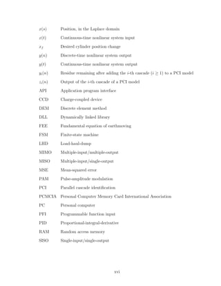
![Chapter 4. Experimental Excavation Studies 40
Structure -
Motion
6
?
Rock pile
Actuators
6
?
-
Pressure
-
Strain
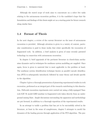
Figure 4.1: A map of the excavation process
as loading proceeded, measured as pressures in the hydraulic cylinders, and;
3. Configuration of the loader mechanism at all times during the loading operation,
measured as hydraulic cylinder extensions and vehicle wheel rotations.
It should be noted that no measurement of the vehicle tractive effort was made,
which technically also contributes to the “Actuators” block of figure 4.1. This follows
directly from the discussion of assumptions given in section 1.2.
Selection and development of the instrumentation and data acquisition systems
necessary to perform the types of measurements listed above was an integral part
of the work performed towards this dissertation. The following subsections disclose
details regarding the loader, instrumentation hardware, and software commissioned
specifically for use during the excavation studies.
4.1.1 Loader Specifications
Full-scale excavation experiments using a Tamrock EJC 9t LHD machine, officially
known as the EJC 1000 prototype [3] and having geometry as shown previously in
figure 1.1 on page 2, were conducted at the facilities of Tamrock Loaders, Inc. of
Burlington ON, Canada. A photograph of the actual trial LHD machine is provided](https://image.slidesharecdn.com/52609fa3-58a5-4f32-9c85-da30edc9900c-150416073852-conversion-gate02/85/Marshall-MScThesis-2001-56-320.jpg)
![Chapter 4. Experimental Excavation Studies 41
Figure 4.2: Photograph of the Tamrock EJC 9t LHD machine
in figure 4.2. The square frame located at the lower right side of the photograph
has outer dimensions 1 yd × 1 yd, included for scale. Table A.12
lists some general
specifications for the Tamrock EJC 9t LHD machine. The machine was equipped with
two lift cylinders (in parallel) and one dump cylinder. The lift and dump cylinder
hydraulic system was an open-center system with one gear pump. Table A.2 gives
some general specifications for the two types of hydraulic cylinders. The cylinders
were operated via a joystick control lever located on the operator console.
The loader was engaged with rock piles of chosen conditions, under the command
of skilled operators, as will be described later in this chapter.
4.1.2 Sensors
This subsection describes the sensors employed to measure the parameters stated
above. The collection of strain gauge data, measuring the mechanical strain at strate-
gic locations on the mechanism boom, was done in order to possibly identify the forces
acting on the mechanism during the loading operation. However, strain gauges were
primarily deployed for the purpose of unrelated, although collaborative, research on
the subject of component loading analysis [64]. Therefore, details regarding the selec-
2
Note that specification data for the hardware discussed in this chapter is, for the most part,
provided in appendix A, in a tabular format.](https://image.slidesharecdn.com/52609fa3-58a5-4f32-9c85-da30edc9900c-150416073852-conversion-gate02/85/Marshall-MScThesis-2001-57-320.jpg)
![Chapter 4. Experimental Excavation Studies 42
tion, configuration, calibration, and commissioning of the strain gauges and related
circuitry are not presented here. Instead, the reader is referred to concurrent related
work by Murphy [64].
Pressure Transducers
In order to allow for computation of the forces at each cylinder during the loading op-
eration, pressure transducers were placed at both head and rod locations on the dump
cylinder and at the same locations on one of the two lift cylinders. Omega Engineer-
ing, Inc. of Stamford CT, U.S.A. models PX303-4KG5V (0–4,000 psig) and PX303-
7.5KG5V (0–7,500 psig) general purpose, gauge-type transducers were installed on
the lift and dump cylinders respectively [1]. Table A.5 gives some specifications for
the employed PX303 series transducers.
Measured pressure transducer voltages were converted into corresponding pres-
sures in Pascals by the relationship
p = a (v − 0.5) (4.1)
where p is the pressure in Pascals (Pa), v is the measured output voltage in volts (V),
and a is a scaling constant such that aL = 6205284 Pa/V for the lift cylinder trans-
ducers (PX303-4KG5V) and aD = 10342140 Pa/V for the dump cylinder transducers
(PX303-7.5KG5V). Corresponding cylinder forces were then computed by subtracting
the force acting at the cylinder rod from the force at the cylinder head, so that
f = pHAH − pRAR (4.2)
where f is the force in Newtons (N), pH and pR are the computed pressures at the
head and rod respectively, and AH and AR are the surface areas (m2
) over which the
pressures at the head and rod acted respectively. The areas needed for equation (4.2)
were computed using rod and bore specifications for the lift and dump cylinders given
in table A.2. Note that, due to the form of equation (4.2), computed cylinder forces](https://image.slidesharecdn.com/52609fa3-58a5-4f32-9c85-da30edc9900c-150416073852-conversion-gate02/85/Marshall-MScThesis-2001-58-320.jpg)
![Chapter 4. Experimental Excavation Studies 43
f were positive if acting so as to extend the cylinder. It is also important to note
that only one of the two lift cylinders was instrumented. Therefore, having made an
assumption that the pressures in both lift cylinders were approximately equal, the
measured lift cylinder force was doubled to represent the combined action of both lift
cylinders in tandem.
Linear Motion Transducers
Since the configuration of the loader mechanism with respect to the vehicle body may
be described completely by two independent coordinates (as will become obvious in
chapter 5), the measurement of only two independent position variables was required.
Two linear motion transducers, in the form of string potentiometers, were used to
record the extension of lift and dump cylinders during the loading operation. Ametek
Aerospace, Gulton-Statham Products of Costa Mesa CA, U.S.A. model P-60A string
potentiometers were employed for this purpose [5]. Table A.6 lists some specifications
for the P-60A linear motion transducer. The transducers were installed in direct line
with the orientation of the lift and dump cylinders.
Online calibrations yielded the expressions
lL = 0.4081 vL + 1.0609 (4.3)
lD = 0.3044 vD + 2.3499 (4.4)
relating the respective lift and dump cylinder lengths lL and lD in meters (m) to
measured potentiometer voltages vL and vD in volts (V).
Wheel Encoder
In order to sense translational motions of the vehicle, a wheel encoder was installed on
the front-right wheel of the trial LHD machine. The encoder was coupled to the tire
via a custom manufactured, spring-loaded wheel follower, shown in the photograph](https://image.slidesharecdn.com/52609fa3-58a5-4f32-9c85-da30edc9900c-150416073852-conversion-gate02/85/Marshall-MScThesis-2001-59-320.jpg)
![Chapter 4. Experimental Excavation Studies 44
Figure 4.3: Photograph of the H25 incremental optical encoder and wheel coupling
mechanism
of figure 4.3. The employed encoder was a BEI Technologies, Inc. of Goleta CA,
U.S.A. model H25D-SS-1000-ABZC-4469-LED-EM18 incremental optical encoder [2].
General specifications for the incremental optical encoder are given in table A.7.
Using the wheel coupling mechanism shown in figure 4.3, the encoder itself was
found to pass through 10.185 rotations per unit rotation of the LHD vehicle tire, which
had a nominal radius of 0.825 m [63]. However, the wheel radius and actual rolling
radius (Rr = 0.796 m) of the LHD vehicle tire differed, since the tire was compressed
slightly due to the machine weight. The lateral distance d, in meters, travelled in the
direction of the LHD vehicle front wheels, assuming no slippage occurred between the
tire and the ground or the tire and the wheel coupling mechanism, was computed as
a function of the encoder cycles per shaft turn (c = 1000) by
d =
2π Rr
10.185 c
= 4.911 × 10⁻⁴
m/count. (4.5)](https://image.slidesharecdn.com/52609fa3-58a5-4f32-9c85-da30edc9900c-150416073852-conversion-gate02/85/Marshall-MScThesis-2001-60-320.jpg)
![Chapter 4. Experimental Excavation Studies 45
Figure 4.4: Workbench photograph of the two SC-2345 shielded carriers with one
opened top, displaying the SCC Series modules within
4.1.3 Signal Conditioning
Conditioning of the voltage signals from the sensors of subsection 4.1.2 was facilitated
through the use of two National Instruments Corporation of Austin TX, U.S.A. SC-
2345 shielded carriers (with configurable connectors and equipped with SCC-PWR03
power modules) in cooperation with a set of off-the-shelf as well as custom fitted
SCC Series modules [67]. In turn, each SC-2345 shielded carrier was connected via
a National Instruments Corporation 68-pin E Series cable (model PSHR68-68) to
a National Instruments Corporation DAQCard-AI-16E-4 16 channel, 12-bit analog,
PCMCIA style personal computer (PC) input device. The two said PCMCIA data
input devices were installed in a Toshiba, Inc. model Satellite 330CT notebook com-
puter, having a Pentium processor, 96.0 MB of random-access memory (RAM), 3.81
GB of data storage space, and running the Microsoft, Inc. Windows 98 4.10.1998
operating system.
For the purpose of strain gauge monitoring, two SCC-SG02, two-channel, 350
Ω, quarter bridge completion modules and four SCC-SG04, two-channel, full bridge](https://image.slidesharecdn.com/52609fa3-58a5-4f32-9c85-da30edc9900c-150416073852-conversion-gate02/85/Marshall-MScThesis-2001-61-320.jpg)
![Chapter 4. Experimental Excavation Studies 46
modules were utilized. Although discussion of the strain gauge instrumentation is
not given here, as per the statement of subsection 4.1.2, it should be noted that the
inclusion of 12 channels of strain gauge measurements is what necessitated the second
SC-2345 carrier and PCMCIA data input device pair.
Three SCC-FT01, two-channel feedthrough modules were customized to provide
buffering, common-mode rejection, and low-pass filtering of sensor signals from the
four pressure transducers and two linear displacement transducers described in sub-
section 4.1.2. A functional circuit diagram for a customized SCC-FT01 module is pro-
vided in figure 4.5. Firstly, differential inputs to each of the two SCC-FT01 module
channels were passed through an Analog Devices, Inc. of Norwood MA, U.S.A. model
AMP04(FP) precision single supply instrumentation amplifier with a chosen gain of
one, set by an external 100 kΩ precision resistor [4]. Having rejected common mode
signals (at approximately 55 dB for unity gain), the resulting ground referenced signal
was then passed through a first-order low-pass filter having a cut-off frequency (de-
fined at −3 dB response) of approximately ωc ≈ 1.6 kHz prior to acquisition by the
data input device. Power was provided to the sensors and signal conditioning com-
ponents via regulated +5 V and ±15 V sources supplied by a SCC-PWR03 power
module located on each of the SCC-2345 carriers.
Digital output from the incremental optical encoder was provided in the form of
two pulse trains, labelled channels A and B, positioned one-quarter cycle out of phase
(i.e. in quadrature) for encoder position and direction measurement. The quadrature
encoder data channels A and B were passed respectively to the PFI8 (source) and
DIO6 (up/down counter 0) pins of a PCMCIA data input device, via the terminal
block provided on the corresponding SCC-2345 carrier unit. A +5 V supply (sourced
from the PCMCIA data input device) referenced to the digital ground pin labelled
DGND was used to power the encoder circuit.](https://image.slidesharecdn.com/52609fa3-58a5-4f32-9c85-da30edc9900c-150416073852-conversion-gate02/85/Marshall-MScThesis-2001-62-320.jpg)
![Chapter 4. Experimental Excavation Studies 47
6
100 kΩ
+15 V
−15 V
3
2
8 100 kΩ
0.001 µF
ACH+
J1-5
J1-6
4
7
5
1
6
100 kΩ
+15 V
−15 V
3
2
8 100 kΩ
0.001 µF
ACH−
J1-1
J1-2
4
7
5
1
SCC-FT01
Notes:
See [67] for SCC-FT01 pad
connection details.
AMP04
1
AMP04
AMP04
+
−
+
−
Figure 4.5: Customized SCC-FT01 feedthrough module circuit diagram](https://image.slidesharecdn.com/52609fa3-58a5-4f32-9c85-da30edc9900c-150416073852-conversion-gate02/85/Marshall-MScThesis-2001-63-320.jpg)
![Chapter 4. Experimental Excavation Studies 48
4.1.4 Data Acquisition Software Programming
Signals were acquired by the twin PCMCIA data input devices described in subsection
4.1.3, and processed on a PC as described in subsection 4.1.3 running a custom built
application in the National Instruments LabVIEW 6i graphical programming envi-
ronment [68, 69]. The commissioned application, entitled LHD-DAQ.vi was written by
the candidate so as to facilitate the collection of data during field trials. The appli-
cation provided a graphical interface for operator input and data visualization pre-
and post-acquisition. User definable options included programmable sensor channels,
buffer size (samples) and scan rate (Hz) selection, in addition to the choice of using
either an ASCII or binary type data storage method.
A sampling of graphical block code for the custom application LHD-DAQ.vi is
depicted in figure 4.6. The portion of graphical code that handled the actual buffered
data acquisition tasks is shown to the left (bottom in figure 4.6), while the remaining
code depicts the data storage function of the application. Notice how the first two
rows of blocks referred to analog signal acquisition from the two PCMCIA input
devices, while the third row dealt with the task of counting rising edges (i.e. digital
signal acquisition) from the incoming incremental optical encoder pulse trains.
4.1.5 Acquisition Synchronization
Synchronization of the two PCMCIA input devices was necessary in order to ensure
that sampling of data from all analog channels, as well as sampling of the digital
counter, was performed simultaneously. To this end, one of the PCMCIA input
devices was designated as a master device, while the other was designated as a slave
device. The analog input “AI scan start” (see figure 4.6) signal was physically routed
via the PFI7 (programmable function input) pin of the master device to the same
pin on the slave device, where it was used as a digital trigger for data acquisition](https://image.slidesharecdn.com/52609fa3-58a5-4f32-9c85-da30edc9900c-150416073852-conversion-gate02/85/Marshall-MScThesis-2001-64-320.jpg)
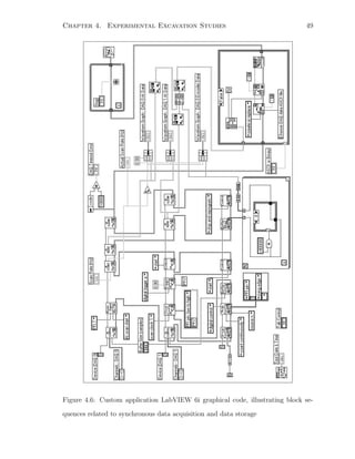
![Chapter 4. Experimental Excavation Studies 50
synchronization. The same signal was also used as a cue for sampling of the counter
value indicating the incremental optical encoder position.
4.1.6 Sampling Rate Selection
A sampling rate of ωs = 3.500 kHz was selected for all trials, mainly to accommodate
the possible high frequency components in strain gauge signals, important to com-
plementary research not discussed in this dissertation [64]. At this rate, according to
the Nyquist criterion [8, page 147], signals with frequencies lower than the Nyquist
frequency ωN = ωs/2 = 1.750 kHz were sampled accurately. Since all of the signal
conditioning modules described in section 4.1.3 included a low-pass filtering stage
with a cut-off frequency at ωc ≈ 1.6 kHz, the possibility of aliasing problems due to
signals with frequency components above ωN was essentially eliminated.
4.2 Experimental Procedures and Observations
In order to acquire operational data representative of the excavation process under
varying, yet controlled, conditions, the instrumented Tamrock EJC 9t LHD machine
was engaged with rock piles (selection was limited) having varying particle size and
composition. Excavation studies were conducted under the command of skilled oper-
ators having moderately varying operating styles, utilizing documented maneuvers.
The following subsections describe fully the chosen trial excavation scenarios and
the degree to which their parameters were known. Finally, a synopsis of the recorded
data and observations is offered, accompanied by some qualitative analysis.
4.2.1 Excavation Trial Scenarios
Each of the excavation trials was conducted in one of two rock pile types, labelled: (i)
local roundstone, and; (ii) Inco muck. The local roundstone consisted of generally fine](https://image.slidesharecdn.com/52609fa3-58a5-4f32-9c85-da30edc9900c-150416073852-conversion-gate02/85/Marshall-MScThesis-2001-66-320.jpg)
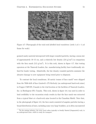
![Chapter 4. Experimental Excavation Studies 52
Figure 4.8: Photograph of the trial rock labelled Inco muck (with 1 yd × 1 yd frame
for scale)
in an underground mining excavation scenario. The muck itself consisted of a fine- to
medium-grained, porphyritic amphibole/biotite rich rock known as amphibolite [54].
The executed excavation scenarios were, for the most part, of one of the following
two categories: (i) controlled excavation trials, or; (ii) aggressive excavation trials.
Controlled excavation trials were conducted by a single operator, where a predeter-
mined sequence of mechanism actions was prescribed. For example, one prearranged
controlled excavation operation kept to the following sequence of steps:
1. Advance loader into the rock pile, with bucket in ready position;
2. Roll back with dump cylinder only, while applying constant tractive effort, and;
3. Retreat from the rock pile upon completion.
A variety of controlled excavation trials were conducted in both local roundstone and
in Inco muck, so as to observe the effects of both rock pile types on the operational
parameters measured by the installed instrumentation.
Aggressive excavation trials were conducted by two skilled operators, different
from the single operator used for the controlled excavation trials. For these aggres-
sive excavation trials, the operators were simply instructed to fill the loader bucket](https://image.slidesharecdn.com/52609fa3-58a5-4f32-9c85-da30edc9900c-150416073852-conversion-gate02/85/Marshall-MScThesis-2001-68-320.jpg)
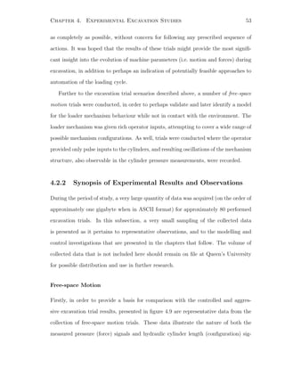
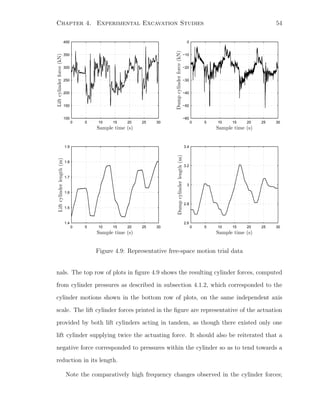
![Chapter 4. Experimental Excavation Studies 55
fluctuations not seen in the relatively smooth cylinder displacements. Observed force
spikes, and subsequent oscillations, in the cylinders corresponded to sudden changes
in motion, for example, an abrupt stop or change in direction. Also, due to the ar-
rangement of the loader mechanism components and actuators, lift and dump cylinder
forces were not independent of one another. For reasons that will be reviewed later
in this thesis, but which are rather obvious, the lift and dump cylinder forces de-
pended not only on their respective cylinder lengths, but on the overall configuration
of the mechanism. For instance, one could not change the lift cylinder length with-
out observing changes in both the lift and dump cylinder forces, although the dump
cylinder length may not have measurably changed. Another particular phenomenon
that was observed, although not illustrated in figure 4.9, was the extremely high force
produced when a cylinder had reached an extension limit. Hitting the stops, as it was
termed, often resulted in a cylinder force exceeding 4–5 times the nominal.
Controlled Excavation
In the consideration of controlled excavation trials, it was learned that there exist
primarily two operator approaches, with regards to lift and dump cylinder actions, to
tackling the fragmented rock excavation problem using an LHD machine. The first
approach is to attack the rock pile using both the boom and bucket actuators, raising
the boom using the lift cylinders whilst rolling back the bucket by retracting the
dump cylinder. The second approach, endorsed by the trial LHD machine manufac-
turer Tamrock Loaders, Inc. [87], aims to utilize only the dump cylinder during the
excavation operation, while decisions on how to actuate the dump cylinder are made
based on the operator perceived excavation conditions. Obviously, in order to fill the
bucket completely and effectively, a significant amount of tractive effort is required,
although this parameter was assumed to be approximately constant for the current
research (again, see section 1.2).](https://image.slidesharecdn.com/52609fa3-58a5-4f32-9c85-da30edc9900c-150416073852-conversion-gate02/85/Marshall-MScThesis-2001-71-320.jpg)
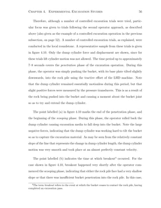
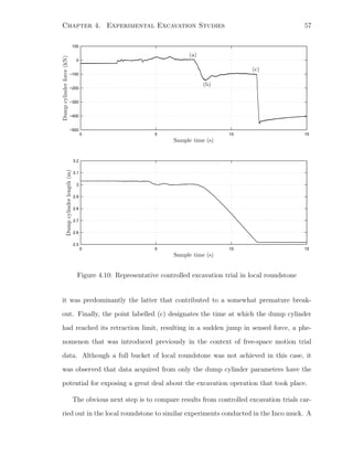
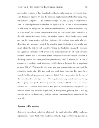
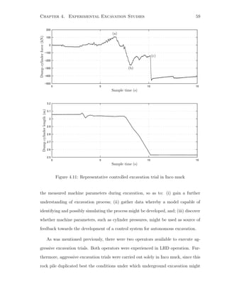
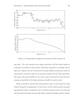
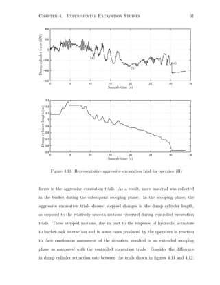
![Chapter 4. Experimental Excavation Studies 62
During controlled excavation trials, a retraction rate of about 140 mm/s was observed,
while during aggressive excavation trials, a reduced cylinder retraction rate closer to
approximately 35–40 mm/s was noted.
For the cases portrayed in figures 4.12 and 4.13, both operators managed to fill the
loader bucket completely. Although both operators utilized only the dump cylinder
during excavation, there were some noticeable differences between their individual
approaches. During the penetration phase, the angle of attack taken by operator (II)
was steeper (longer dump cylinder length) than that used by operator (I), resulting
in relatively high forces experienced by the dump cylinder during penetration of the
rock pile. Although the cylinder displacement plot for operator (I) indicates that a
stepping action was used during retraction of the cylinder in the scooping phase, the
cylinder displacement plot for operator (II) indicates the use of significant oscillations,
perhaps in an attempt to fluidize the rock pile so as to cause rock particles to flow
more easily in and around the bucket. This type of action, causing oscillation of the
bucket angle, is reminiscent of the algorithm described by the patent of Dasys et
al. [15], mentioned in chapter 2. For the case shown in figure 4.12, operator (I) was
able to keep the bucket within the rock pile for almost the entire time dump cylinder
retraction was taking place. Whereas, operator (II) was able to break out of the pile
at an earlier stage of dump cylinder retraction (although it took approximately the
same time to pass from point (a) to point (b) in both cases).
At the very least, the aggressive excavation trials have allowed for qualitative and
comparative observations to be drawn regarding the excavation of fragmented rock
using an LHD machine. Through the collection and analysis of operational data, a
clearer understanding of the excavation process and its characteristic stages has been
achieved. It is these data that provide the basis for further study in the chapters that
follow.](https://image.slidesharecdn.com/52609fa3-58a5-4f32-9c85-da30edc9900c-150416073852-conversion-gate02/85/Marshall-MScThesis-2001-78-320.jpg)
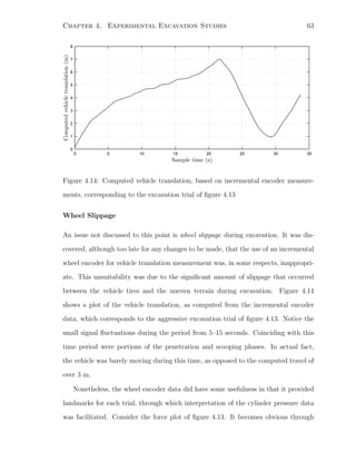
![Chapter 5. Dynamics of the Loading Process 66
tions in fragmented rock, using the parallel cascade identification (PCI) technique.
Data from aggressive full-scale experimental trials, as described in chapter 4, were
used in the identification process for linear and nonlinear elements of PCI models.
Attempted modelling scenarios are provided alongside a detailed description of the
means by which the PCI algorithm was implemented and applied.
5.1 Euler-Lagrange Formulation
A first attempt at modelling the loader mechanism dynamics (as an exercise in applied
mechanics) was done without concern for rock interaction, and through consideration
of the mechanism as a robot manipulator, similar to the concepts proposed in [33, 86].
Concurring with the experimental material of chapter 4, only the dynamics resulting
from lift and dump cylinder actuation were considered. A Lagrangian approach, as
described in chapter 3, was used to derive equations of motion for the given mecha-
nism. This was also recognized by Sarata et al. [86]. However, in [86], only a means
through which the equations might be formulated was given, and the technique was
never actually implemented.
The loader mechanism of the Tamrock EJC 9t LHD machine used for the current
research, by inclusion of the linear actuators, formed a multi-loop, closed kinematic
chain of links. It is conceivable that dynamical equations of motion could have been
formulated using only the boom and bucket links of the system, through the applica-
tion of actuator forces as external forces on the resulting serial mechanism. Although
this more simplistic perspective might have been acceptable for static force analysis
[33], the inertial properties of the actuators and the inclusion of explicit holonomic
constraints that define the closed kinematic chains shaped a convincing argument for
an attempt at formulation of the system as a closed-chain mechanism.
Schematic drawings of the Tamrock EJC 9t LHD loader mechanism are presented](https://image.slidesharecdn.com/52609fa3-58a5-4f32-9c85-da30edc9900c-150416073852-conversion-gate02/85/Marshall-MScThesis-2001-82-320.jpg)
![Chapter 5. Dynamics of the Loading Process 67
PSfrag replacements
E
B
C
D
A
F
ql
qd
τl
τd
Figure 5.1: Schematic drawing of the loader mechanism
in figures 5.1 and 5.2. The actuated lift and dump cylinder prismatic joints were
denoted by ˜q = [ql qd]T
∈ 2
and the corresponding actuated cylinder forces denoted
by ˜τ = [τl τd]T
∈ 2
. Table A.3 (located in appendix A.1 on page 134) lists the
inertial properties1
for each of the links in the system. Note that, although the boom
and bucket links were obviously much larger in mass than the actuators, the cylinder
component masses themselves were not entirely insignificant. Table A.4 lists the fixed
physical dimensions of the loader mechanism, as illustrated by figure 5.2.
5.1.1 Reduced System Mechanics
As was necessary, the loader mechanism of figure 5.1 was cut open at strategic boom
and dump cylinder locations; namely points E and F. The dynamics of the serial
reduced system were then modelled through an application of the Euler-Lagrange
equations, as described in chapter 3. The Denavit-Hartenberg [16] coordinate frames
for the serial reduced system were developed, as shown in figure 5.3, and the joint
1
Moments of inertia Izzi were taken about the link centre of mass, with reference to the base
frame. The constants aci and bci were used to locate the centre of mass of link i. Values were
computed through computer modelling of the boom and bucket structures; see [64].](https://image.slidesharecdn.com/52609fa3-58a5-4f32-9c85-da30edc9900c-150416073852-conversion-gate02/85/Marshall-MScThesis-2001-83-320.jpg)
![Chapter 5. Dynamics of the Loading Process 68
E
B
C
D
A
Fd6
d7
d2
d1
d3
d5
d4
Figure 5.2: Fixed physical dimensions of the loader mechanism
variables were subsequently denoted by q = [q1 . . . q6]T
∈ 6
, with q2 and q6 being
linear displacements corresponding to the lift and dump cylinder extensions. The
corresponding generalized actuating forces were denoted by τ = [τ1 · · · τ6]T
∈ 6
.
Kinetic and Potential Energy Expressions
The total kinetic energy of the reduced system was written as
K =
1
2
6
i=1
mivT
civci + ωT
i Iiωi =
1
2
˙qT
D(q) ˙q (5.1)
with
vci = Jvci
(q) ˙q (5.2)
ωi = RT
i (q)Jωi
(q) ˙q (5.3)
for i = 1, 2, . . . , 6 links, where Jvci
(q) and Jωi
(q) were Jacobian matrices, the matrix
Ri(q) took care of the fact that the angular velocity ωi must be expressed in a frame
attached to its respective link, and Ii was the inertia tensor for the link i about its](https://image.slidesharecdn.com/52609fa3-58a5-4f32-9c85-da30edc9900c-150416073852-conversion-gate02/85/Marshall-MScThesis-2001-84-320.jpg)
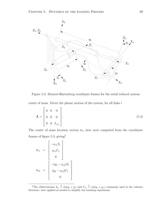
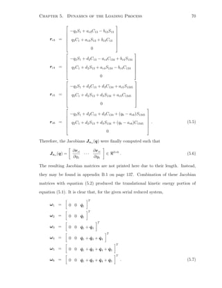
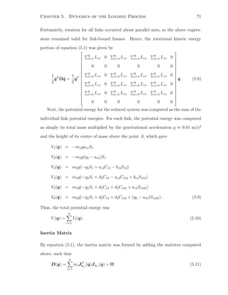
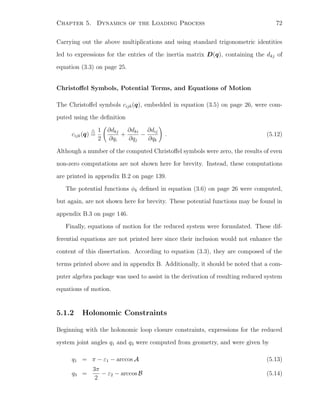
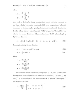
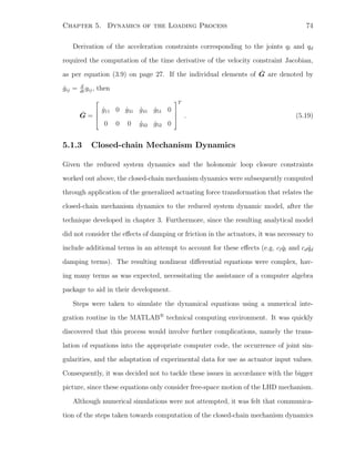
![Chapter 5. Dynamics of the Loading Process 75
was a worthwhile exercise, as well as complementary to the problem at hand.
5.2 Modelling Alternatives
The analytical approach of section 5.1 considered modelling only the LHD loader
mechanism, without consideration for any interaction with its environment, namely
a rock pile. In order to have any usefulness towards the problem of autonomous
excavation, the given analytical model would have to be extended to include external
forces acting on the bucket link. From a mechanical system modelling perspective,
this extension would be relatively straight forward in that generalized forces, more
specifically their corresponding influence on the chosen coordinates, need simply be
appended to the model of section 5.1. This is illustrated in figure 5.4, where fa
represents the vector of externally applied actuator forces, fr denotes the vector of
resistive forces to excavation, and x is the machine state. However, the problem of how
to compute, for the purpose of modelling, the forces of resistance during excavation
remains unresolved. In section 2.2, it was noted that various empirical and analytical
studies have been conducted with the intent of resolving such interaction forces from
a mixed set of excavation parameters. For example, consider the work of Takahashi
et al. [102, 105], where resistive forces during excavation were computed analytically
using assumed geometric and frictional parameters of the bucket and rock pile.
In the subsections that follow, a distinct element method (DEM) and artificial
neural networks are considered briefly as two possible approaches to the problem of
bucket-rock interaction modelling.
5.2.1 Distinct Element Method
The distinct element method (DEM), after Cundall and Strack [14], entails construc-
tion of a numerical model capable of describing the mechanical behaviour of collections](https://image.slidesharecdn.com/52609fa3-58a5-4f32-9c85-da30edc9900c-150416073852-conversion-gate02/85/Marshall-MScThesis-2001-91-320.jpg)
![Chapter 5. Dynamics of the Loading Process 76
fa
- Machine
dynamics
-
x
Bucket-rock
interaction
6
fr
Figure 5.4: A block model for the machine excavation process
of particles, modelled as discs (or spheres in three dimensions). The computational
scheme is based on an application of Newton’s second law to each individual parti-
cle (i.e. disc or sphere), in conjunction with a force-displacement law describing the
particle to particle contact forces. Hence, the force-displacement law is used to find
particle interaction forces from displacements, while Newton’s second law computes
the motion of each particle based on the contact forces that act on it.
In reality, the force-displacement law is meant to represent the deformation of
individual particles while in forced contact with each other. However, for the purpose
of assembly simulation, the particles are simply allowed to overlap one another at
contact points. It should be noted, however, that the magnitude of overlap is to be
very small in comparison with the individual particle sizes. The resulting contact
force is then computed to be in direct proportion with the degree of overlap, as
though there existed a spring-type element, connecting the two particles, that acts
only in compression. Likewise, a damping element may be added to the model, which
again, acts only when the particles are in contact. Models may be constructed to act
similarly in both normal and tangential directions of contact, so as to imitate both
normal and shear forces acting on each particle, although allowing the variation of
parameters to dictate the specific force-displacement relationship in each direction.
For arithmetic details of the algorithm, the reader is referred to [14, 101].](https://image.slidesharecdn.com/52609fa3-58a5-4f32-9c85-da30edc9900c-150416073852-conversion-gate02/85/Marshall-MScThesis-2001-92-320.jpg)
![Chapter 5. Dynamics of the Loading Process 77
As was mentioned in chapter 2, the DEM of Cundall and Strack was conceived
for the purpose of modelling granular assemblies having very small particle sizes, at
least in relation to the fragmented rock piles described in chapter 4. Nonetheless, the
technique was recently applied by Takahashi [101] to simulation of particle behaviour
in a virtual rock pile. Unfortunately, since the experimental data Takahashi used
to validate the DEM model was derived from laboratory scale trials, the constructed
DEM model used a particle diameter of only 12 mm. In addition, the model employed
a uniform particle size, as well as a predetermined (or prescribed) motion for the ex-
cavator bucket. As a result, there remains much room for improvement and extension
of the DEM approach to modelling bucket rock interaction forces. For example, con-
sider the use of a DEM model to act as the block titled “Bucket-rock interaction” of
figure 5.4. Ideally, the Lagrangian model of section 5.1 could be extended, as pre-
viously discussed, and subsequently used as the block titled “Machine dynamics” of
figure 5.4. Through combination of the two models in such a way, the simulations
performed by Takahashi [101] could be appropriately extended to include the machine
dynamics, and the fact that a system for autonomous excavation would necessitate
determining the required actuator inputs to overcome bucket-rock interaction forces.
Further to including the machine dynamics, the DEM model could be improved
by selecting assemblies of particles having varying sizes, as is typical to the aver-
age fragmented rock pile. In fact, there exist already well established techniques for
describing particle size distributions for piles of fragmented rock. For example, the
Rosin-Rammler equation has been used for blasting analysis [38], which uses tech-
niques from the field of mineral dressing, and has the form
R = 1 − e−(ds
dc
)
n
(5.20)
where R is the fraction of material less than the diameter ds, the constant dc is called
the characteristic size, and n is a constant called the uniformity index. Therefore,
through adjustment of the characteristic size and uniformity index parameters, var-](https://image.slidesharecdn.com/52609fa3-58a5-4f32-9c85-da30edc9900c-150416073852-conversion-gate02/85/Marshall-MScThesis-2001-93-320.jpg)
![Chapter 5. Dynamics of the Loading Process 78
ious rock pile distributions could be developed, possibly based on actual rock pile
measurements, for use in defining a collection of particles to be employed in DEM
modelling.
Integration of the above suggested improvements with the available experimental
data reported in chapter 4 could provide one alternative to modelling the excavation
process. However, some disadvantages of the DEM approach include its numeri-
cally intense nature, and the fact that the technique would only be useful in offline
simulations, providing little additional knowledge that might be incorporated into a
potential controller for autonomous excavation.
5.2.2 Artificial Neural Networks
Another possible approach to modelling the excavation process, whether simply the
LHD loader mechanism or the entire excavation process, lies in the application of
artificial neural networks. Such neural networks refer to the formulation of systems
whose central theme is borrowed from the analogy of biological neural networks [60].
Essentially, artificial neural networks, similar to biological neural networks, consist of
an interconnected collection of nodes (analogous to neurons), where each node per-
forms some simple computation over its inputs, or more commonly over the sum of
its inputs. Inputs (analogous to synapses) are in turn weighted (analogous to synap-
tic efficiency) and interconnected based on the desired network function, through a
training (analogous to learning) procedure.
Perhaps the most common of the artificial neural network architectures is the mul-
tilayer feedforward network where training is accomplished through application of the
least mean squared algorithm known as backpropagation, popularized by Rumelhart
et al. [83]. In the context of applied science and engineering, such artificial neural
networks have been utilized for robot control, vehicle control, and even the identi-
fication of robot inverse kinematics [60]. In fact, in their work, Shi et al. [90, 91]](https://image.slidesharecdn.com/52609fa3-58a5-4f32-9c85-da30edc9900c-150416073852-conversion-gate02/85/Marshall-MScThesis-2001-94-320.jpg)
![Chapter 5. Dynamics of the Loading Process 79
employed the backpropagation algorithm to the problem of autonomous excavation,
by training their finite-state machines (see section 2.1) for individual tasks based on
data collected from observed human operator actions.
Advantages of the artificial neural network approach, in the task of modelling
nonlinear systems, lie in its intrinsic simplicity and the ease by which training of
the network may be accomplished. There exist, however, several difficulties and
disadvantages to the use of neural networks. Firstly, selection of the network structure
(i.e. number of layers and nodes per layer) is often arbitrary, often selected by trial
and error. Secondly, there exist issues surrounding error convergence to a global
minimum and the ability of a given network to generalize. Perhaps most notably,
once a network has been developed and identified, there exist no real means by which
significance may be attributed to its structure or the values of its connection weights,
providing little insight as to the physical nature of the identified process.
5.3 Parallel Cascade Identification
It was decided that an effort to employ the method of parallel cascade identification
(PCI) for nonlinear systems might be a worthwhile mission, since the system to be
modelled (i.e. the observed excavation process) seemed to fit the criteria communi-
cated by Korenberg in [44]. Furthermore, it had been reported recently that a SISO
version of the PCI algorithm had been used successfully by Eklund and Korenberg
[19, 20] to simulate aircraft pilot flight controls, having a dynamic model similar in na-
ture to the LHD loader mechanism. Although the analytical model used to represent
the flight control system used by Eklund and Korenberg [20, page 74] was markedly
less complex than the system described by the proposed Euler-Lagrange equations
of section 5.1, it was noted that the PCI algorithm had no troubles identifying even
significant hysteresis nonlinearities [19, page 83] in the system.](https://image.slidesharecdn.com/52609fa3-58a5-4f32-9c85-da30edc9900c-150416073852-conversion-gate02/85/Marshall-MScThesis-2001-95-320.jpg)
![Chapter 5. Dynamics of the Loading Process 80
Moreover, as opposed to the DEM and artificial neural network approaches de-
scribed in the previous section, a PCI model that could describe the LHD loader
mechanism and resulting bucket-rock interactions would have a known internal struc-
ture, and hence yield information that might be exploited towards the development
of a control system for autonomous excavation. At the very least, an accurate and
easily applicable tool would become available for analysis and possibly simulation
during controller design.
5.3.1 Algorithm Implementation
A multiple-input/single-output (MISO) version of the PCI algorithm was imple-
mented in the C programming language on a PC having a 450 MHz Pentium II
processor and 384 MB of RAM. The C language code was compiled, using a Microsoft
6.0 C/C++ compiler, and called as a dynamically linked library (DLL) for use in the
MATLAB
r
(version 5.3.129215a, release 11.1) technical computing environment, via
a proprietary MATLAB application program interface (API). The reason for the use
of a C language routine, or so-called C language MEX-file [58], was to circumvent
the severe computational bottlenecks (e.g. while- and for-loops) that do not run
fast enough in MATLAB. The resulting C language MEX-file was named suitably
PCI.dll.
For the most part, the PCI algorithm was coded as it was described previously, in
chapter 3, and in the manner published by Korenberg [44]. However, there were some
extensions included in the final implementation, not mentioned in chapter 3, which
should be noted. Firstly, up to third-order cross correlations were employed (the
flight control system model of Eklund and Korenberg [19, 20] was found to require
only first-order cross-correlations), resulting in the use of
φxxxyi−1
(j1, j2, j3) = yi−1(n)x(n − j1)x(n − j2)x(n − j3) (5.21)](https://image.slidesharecdn.com/52609fa3-58a5-4f32-9c85-da30edc9900c-150416073852-conversion-gate02/85/Marshall-MScThesis-2001-96-320.jpg)
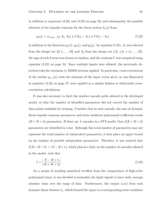
![Chapter 5. Dynamics of the Loading Process 82
element Ni, was also scaled to have unity average absolute value over the interval
n = R, (R+1), . . . , T, after the example of Eklund and Korenberg [20]. These scaling
procedures were necessary in particular when the inputs to the system to be identified
were hydraulic cylinder forces, having a magnitude on the order of 105
N.
It is often the case that a model may be improved by including recently past
values of the output as an additional input signal. For example, if a system has an
input x(n) and an output y(n), a new model may be constructed that has two inputs,
namely x1(n) = x(n) and x2(n) = y(n − 1), and one output y(n) [44]. The option
to extend the algorithm to perform this function was incorporated into the PCI.dll
routine. However, it should be noted that stability of the resulting model was found
to be no longer guaranteed with the inclusion of output feedback, as one might have
expected. Therefore, to reduce the chance of possible instability, the polynomial order
was limited to a maximum of M = 2 for cascades that utilized a time delay of the
output as input.
Since the intended function of the modelling process was to identify a general
model for the system at hand, and not simply memorize a particular set of in-
put/output data, the option was provided in the PCI.dll routine to include mul-
tiple data sets for training, as is typical in the training of artificial neural networks.
This was done by inserting marker points (specifically, data points having a value of
1 000 000) between distinct data sets, which the routine used to recognize the start
of a new data set and when to subsequently jump (R + 1) steps forward in time.
While the C language code that forms the source for PCI.dll is not fully dis-
closed in this dissertation (as it totalled over 900 lines), the pseudo-code of figure
5.5, written in a C programming style, illustrates the elementary framework of the
C language MEX-file source code for the described PCI.dll routine. The ellipses
“...” mark the omission of large segments of code not necessary to understanding
the intended general message of the figure. Note that the while-loop was allowed](https://image.slidesharecdn.com/52609fa3-58a5-4f32-9c85-da30edc9900c-150416073852-conversion-gate02/85/Marshall-MScThesis-2001-98-320.jpg)
![Chapter 5. Dynamics of the Loading Process 83
to continue until either the computed model MSE (denoted e) was less than some
desired MSE threshold (denoted MSE), the maximum number of possible cascades had
been exceeded, or the number of tried cascade candidates had exceeded 500. It was
typical in practice to set the fixed value of MSE to a sufficiently small number, so as to
allow the algorithm to try a significant number of possible cascade candidates during
system identification.
Once the source code had been compiled as a MEX-file for MATLAB, it was avail-
able for use as a function from within the MATLAB technical computing environment.
The calling syntax for PCI.dll from within MATLAB was
[yApci,yBpci,mseA,mseB,I] = pci(xA,yA,xB,yB,MSE,R,M)
where xA and xB were the matrices composed of input vectors for training and test-
ing respectively, yA and yB were the vectors of output data for training and testing
respectively, MSE was the target mean-squared error3
, the integers R and M were the
specified memory length and polynomial order respectively, yApci and yBpci were
the identified PCI model outputs for training and testing respectively, mseA and mseB
were the computed mean-squared errors for training and testing, and I was the num-
ber of cascades in the identified model. Note that PCI.dll was intended only to
implement the PCI algorithm for the purpose of validating the application of PCI to
modelling of the LHD loader mechanism and possibly the excavation process. Mod-
ifications and/or further coding would be required in order to extract the identified
model parameters for subsequent simulations.
Prior to use in modelling of the LHD loader mechanism and the excavation process,
the PCI.dll routine was tested on a contrived data set, representative of an invented
nonlinear system. The test system was a MISO nonlinear difference equation, derived
through modification by the candidate of a SISO nonlinear difference equation that
3
In all cases, mean-squared error was computed as a percent of the output signal span.](https://image.slidesharecdn.com/52609fa3-58a5-4f32-9c85-da30edc9900c-150416073852-conversion-gate02/85/Marshall-MScThesis-2001-99-320.jpg)
![Chapter 5. Dynamics of the Loading Process 84
#include mex.h // Include the MATLAB MEX-function header.
void pciFunction( ... )
{
/* The function pciFunction() performs parallel cascade
identification, building a model based on the algorithm. */
int i = 0; // Cascade counter.
int stop = 0; // Iteration counter.
/* Add parallel cascades while conditions are satisfied. */
while( ( e MSE ) ( i (R + M + 2)/(T - R + 1) )
( stop 500 ) ) {
i++; // Increment the cascade counter.
stop++; // Increment the iteration counter.
/* For each time delay find a delta response. */
for( r = 0; r (R + 1); r++ ) {
... ;
}
/* Compute polynomial coefficients. */
for( m = 0; m (M + 1); m++ ) {
... ;
}
/* Check statistical benefit of cascade. */
e = ... ;
if( benefit == false )
i--; // Decrement the cascade counter.
}
}
void mexFunction( int nlhs, mxArray *plhs[],
int nrhs, const mxArray *prhs[] )
{
/* The function mexFunction is the gateway (application
program interface) routine for MATLAB. */
... ;
}
Figure 5.5: Pseudo-code illustrating the elementary structure of the C language MEX-
file written to implement PCI for use in MATLAB](https://image.slidesharecdn.com/52609fa3-58a5-4f32-9c85-da30edc9900c-150416073852-conversion-gate02/85/Marshall-MScThesis-2001-100-320.jpg)
![Chapter 5. Dynamics of the Loading Process 85
was borrowed by Korenberg [44, page 443] from McIlroy [59], who employed the
said difference equation to model a simulated communications channel. The newly
invented system, with input x(n) = [x1(n) x2(n)]T
, was the nonlinear difference
equation
y(n) = −0.636507 + 1.08717x2(n − 24) + 0.914799x2
1(n − 23)
− 0.698645x2(n − 27) + 0.967739x2
2(n − 25) + 0.787682x1(n − 22)
− 0.630834x3
1(n − 28) + 0.160929x2(n − 30) − 0.209741x2(n − 32)
+ 0.397268x5
1(n − 21) − 0.117377x1(n − 29) − 0.49215y(n − 2)
+ 0.114922y2
(n − 5) + 0.129476x1(n − 24)x1(n − 23)
+ 0.211136y2
(n − 1) − 0.152675x2(n − 24)y(n − 6) . (5.24)
Using inputs chosen arbitrarily to be of the form
x1(n) = sin(0.05n) cos(0.0808n − 0.052) (5.25)
x2(n) = sin(0.033n) sin(0.025n − 0.08) (5.26)
for n = 1, 2, . . ., two sets of input/output data were computed, for training and
testing, each 1000 points long. The two sets were then passed as arguments, along
with various combinations of memory length and polynomial order, to the PCI.dll
routine.
Figure 5.6 shows4
the outcome of one attempt to model the contrived system using
equations (5.25) and (5.26) as inputs, plus output feedback. The resulting model had
22 cascades, each with a memory length R = 35 and a polynomial order M = 5
(except those with output feedback, where the polynomial order was restricted to
M = 2). The computed MSE for the training data shown in figure 5.6(a) was 0.0457
% over the output span, and the corresponding MSE for the testing data shown in
figure 5.6(b) was 0.1382 %. In fact, modelling outcomes were generally successful
4
In all such figures, the dashed line denotes the PCI model output.](https://image.slidesharecdn.com/52609fa3-58a5-4f32-9c85-da30edc9900c-150416073852-conversion-gate02/85/Marshall-MScThesis-2001-101-320.jpg)
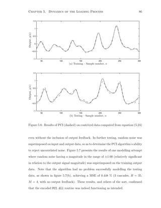
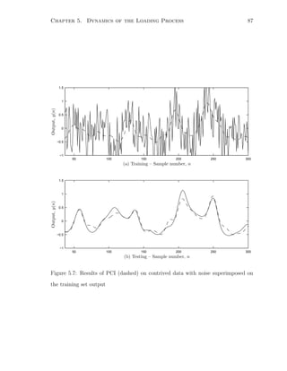
![Chapter 5. Dynamics of the Loading Process 89
reasoning behind this was twofold: (i) in view of Newton’s Second Law, one might
expect input forces to be more directly related to velocity as opposed to position,
and; (ii) integration of resulting motions seemed to provide a more smooth and con-
sistent result for comparison with the measured position data. Therefore, prior to
system identification, the derivative of position data was computed using a first-order
finite divided difference approximation [11, page 93]. Subsequent integrations were
performed by a cumulative trapezoidal numerical integration routine [11, page 478].
The inverse dynamics problem was not considered since for the data collected,
if one presumes that it is the application of cylinder forces that results in cylinder
motions and not the converse, this situation would represent a system that is not
causal in nature. However, for the aggressive excavation trials, it is entirely plausible
that external forces on the mechanism result in motions of the boom and bucket
links (no matter how small), which in turn cause possibly significant changes in the
measured cylinder forces. In fact, it is this postulate that forms a basis for the
reactive control schemes proposed in the reviewed patents [15, 77] of chapter 2. By
this rationale, the PCI algorithm may not be as applicable as originally thought.
5.3.3 Synopsis of Identification Results and Observations
During this research, various other modelling scenarios were also attempted. Nev-
ertheless, the described scenarios (A) and (B) of the previous subsection provided
sufficient results for the purposes of this dissertation.
Scenario (A): Forward Dynamics in Free Space
The free-space motion trial data of section 4.2.2 was employed to fit PCI models
using the PCI.dll routine under the definition of scenario (A). The results of one such
attempt at modelling of the lift cylinder motions is shown in figure 5.8(a), subsampled](https://image.slidesharecdn.com/52609fa3-58a5-4f32-9c85-da30edc9900c-150416073852-conversion-gate02/85/Marshall-MScThesis-2001-105-320.jpg)
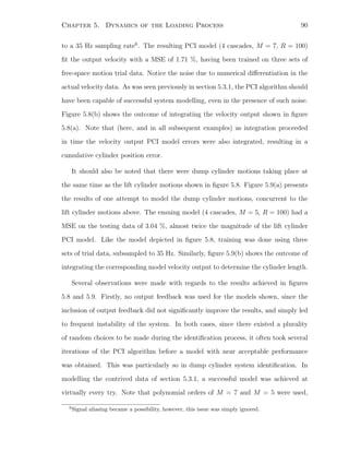
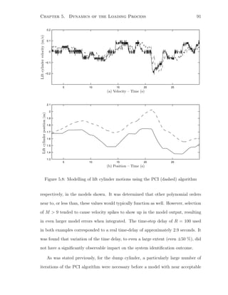
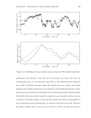
![Chapter 5. Dynamics of the Loading Process 93
four-bar linkage mechanism, causing the dump cylinder to depend more heavily on
the configuration of the boom and bucket links combined. This train of thought led
to contemplation of the possibility that PCI might be, in some respects, unsuitable
to the problem at hand. This is discussed further in section 5.3.4. Nonetheless, it
may be possible that PCI, with other variations and combinations in the parameters
M,R, sampling rate, total number of samples, and number of training sets, might
yield better results [45].
Scenario (B): Aggressive Excavation
Despite the fact that the free-space motion modelling of scenario (A) was only mod-
erately successful, and that an attempt to include bucket-rock interactions into the
equation would not likely improve the situation, modelling of the excavation pro-
cess was attempted as per the definition of scenario (B). As was discussed in sec-
tion 4.2.2, operators (I) and (II) had similar styles in that they chose to use only
the dump cylinder, in combination with tractive effort, during aggressive excavation
trials. Hence, figure 5.10 shows the outcome of one attempt to identify the excava-
tion process through dump cylinder motions. The resulting PCI model (7 cascades,
M = 6, R = 10) was again trained using three data sets, and tested on a fourth. The
computed MSE on the testing data velocity output was a surprising 1.99 %. One
possible reason for the relatively good result is that only the dump cylinder was used
by the operator, as opposed to the command of a range of lift and dump cylinder
motions, as was the case in scenario (A).
Identification of the aggressive excavation trials differed from the free-space motion
trials above in that modelling success was found to be somewhat sensitive to the time-
delay. The comparatively short time-delay (approximately 0.3 seconds) indicates that
essentially present values of the cylinder forces were identified as being responsible
for the motions shown. This makes some sense in that force/motion changes occurred](https://image.slidesharecdn.com/52609fa3-58a5-4f32-9c85-da30edc9900c-150416073852-conversion-gate02/85/Marshall-MScThesis-2001-109-320.jpg)
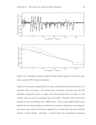
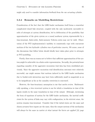
![Chapter 5. Dynamics of the Loading Process 96
89]. Therefore, the time-invariancy restriction for Volterra series representations is
obeyed.
Nevertheless, there does remain one potentially serious issue. If the given mech-
anism is started in one particular configuration and a unique set of actuator inputs
is applied, then a specific motion of the system would result. Then again, if the
mechanism is started in a different configuration and the same unique set of actuator
inputs is applied, then presumably different motions of the system would result. This
is mainly due to the dependance of inertial and gravitational characteristics of the
mechanism on its configuration. Therefore, in this sense, the outputs of the system
will always depend on the initial conditions, a characteristic of systems possessing
infinite memory7
. This revelation might help to understand the results of subsection
5.3.3. From a qualitative viewpoint, the outcome of lift cylinder free-space motion
modelling was most definitely better than similar attempts at modelling the dump
cylinder motions. This observation might be rationalized by appreciating that lift
cylinder motions were less dependent on the initial conditions, since the cylinder it-
self passed through only small changes in position and orientation in space. This
was certainly true in comparison with motions of the dump cylinder, which formed
one branch of a four-bar linkage system. As was noted previously, the results of
modelling the dump cylinder motions while in contact with the rock pile were un-
expectedly good. Though, this may be attributed to the fact that the lift cylinder
was not moved at all during these trials, it is perhaps more due to the fact that
motions of the dump cylinder were started at essentially the same configuration and
passed through almost the same trajectory at each excavation iteration during model
training.
In comparison with PCI modelling results corresponding to the contrived data
of subsection 5.3.1, as well as its performance as reported by Eklund [19, 20], the
7
However, this is not to imply that the system has infinite memory in the sense of its inputs.](https://image.slidesharecdn.com/52609fa3-58a5-4f32-9c85-da30edc9900c-150416073852-conversion-gate02/85/Marshall-MScThesis-2001-112-320.jpg)
![Chapter 6
An Excavation Control Design
As was discussed in chapter 2, the control problem in autonomous excavation evi-
dently requires an approach that is different than any of the well known strategies for
trajectory control of industrial robot manipulators. Hemami [27] suggested that the
excavator bucket trajectory should not have priority in the chosen control scheme,
since the objective is to fill the bucket, and not follow some strictly specified path. The
problem is further compounded by the complex nature of bucket-rock interactions,
which result in the need for an innovative approach to automating the excavation pro-
cess. Also, it was discussed in chapter 1 how the autonomous excavation problem may
be regarded in its broadest sense to include the challenge of planning a higher-level
excavation goal (e.g. excavate a particular area of specified size or volume). However,
in this chapter, consideration is not given to the problem in this general sense. Rather,
the problem was defined as one of how to select the appropriate actuator inputs so as
to control the motion of the LHD loader mechanism to fill its bucket completely and
reliably, without any need for operator intervention. Furthermore, only the scooping
phase of excavation is considered within the problem scope, as it corresponds with
relevant observations made from full-scale excavation and modelling studies.
Though the explicit mathematical formulation and implementation of a control
98](https://image.slidesharecdn.com/52609fa3-58a5-4f32-9c85-da30edc9900c-150416073852-conversion-gate02/85/Marshall-MScThesis-2001-114-320.jpg)
![Chapter 6. An Excavation Control Design 99
system for autonomous excavation of fragmented rock lies outside the scope of this
dissertation, it was decided that formulation of a controller design concept, based
on observations from experimental studies and modelling, would be a worthwhile
contribution. Such is the intent of this chapter, which proposes the use of ideas from
the field of compliant motion control.
6.1 Compliant Motion Control for Excavation
Controlling the mechanical interaction between a robot manipulator and its envi-
ronment, such as in manufacturing assembly operations, has been a topic of many
discussions in the robotics and control literature. The conceded shortcomings of pure
position control in situations where environment interaction must take place have
led to the development of techniques for control that lie generally under the label
of compliant motion control, or sometimes force control [36, 39, 75, 98, 108]. Con-
sider the classic example of a window-washing robot, where slight deviations in the
manipulator trajectory under pure position control might cause the tool to lose con-
tact with the window surface, or perhaps result in extremely large contact forces and
impending disaster. Rather than attempt to follow a strictly specified trajectory,
compliant motion control techniques are generally concerned with not only follow-
ing a prescribed trajectory, but directly regulating the forces of interaction between
the manipulator and its environment. One method, termed impedance control [36],
focuses on the relationship between the manipulator velocity and the forces of inter-
action with its environment, a relationship that is typically referred to as mechanical
impedance. In the Laplace domain, mechanical impedance Z(s) may be represented
(in one dimension) by the relation
Z(s) =
f(s)
v(s)
(6.1)](https://image.slidesharecdn.com/52609fa3-58a5-4f32-9c85-da30edc9900c-150416073852-conversion-gate02/85/Marshall-MScThesis-2001-115-320.jpg)
![Chapter 6. An Excavation Control Design 100
where f(s) is the environment interaction force and v(s) is the manipulator tool
(e.g. LHD bucket) velocity at the point of contact with the environment [98]. It is the
task of an impedance controller to produce a response of the mechanism that corre-
sponds to some prescribed impedance Z(s). Therefore, impedance control considers
the manipulator as a mechanical impedance, while the environment with which it is
coupled is considered as a mechanical admittance. As one might expect, mechanical
admittance Y (s) may be represented by the relation
Y (s) =
v(s)
f(s)
(6.2)
which is in fact the reciprocal of mechanical impedance [70, 89]. Hence, impedances
may be seen as systems that accept motion and respond with a force, while admit-
tances as systems that accept force and respond with motion. Hogan [36] argued that,
as seen from the manipulator, the environment must be considered as a mechanical
admittance, and not an impedance, since kinematically constrained inertial objects
(e.g. a window) can always be pushed on, but cannot always be moved. Typical
impedance control implementations have focused on either model-based computation
of the joint and/or actuator torques necessary for a manipulator to follow a given
impedance characteristic [36, 98], or on position-based impedance controlled manip-
ulators [72].
The concept of impedance control has been considered already as one possible
approach to controller development for excavation related tasks. Researchers at the
University of British Columbia [18, 84, 85] incorporated impedance control into the
tele-operation of a miniature backhoe style excavator. As was discussed in chapter
2, Bernold [9] proposed that the use of impedance control (in the excavation of soil
type media) would permit the assignment of a target relationship between the actual
position of the excavator bucket and its desired position according to some planned
nominal path. Also, Ha et al. [26] have recently proposed the implementation of an
impedance control scheme for backhoe excavation bucket trajectory following.](https://image.slidesharecdn.com/52609fa3-58a5-4f32-9c85-da30edc9900c-150416073852-conversion-gate02/85/Marshall-MScThesis-2001-116-320.jpg)
![Chapter 6. An Excavation Control Design 101
However, the above impedance control schemes imply that there exists some pre-
determined nominal trajectory that the excavation bucket should follow. In the case
of tele-operation, this trajectory would presumably come from the command of a re-
mote operator. On the other hand, for autonomous excavation, the path the bucket
should follow is not entirely clear, since the ultimate objective is to fill the bucket
and not to follow some prearranged trajectory.
6.2 Re-examination of the Control Problem
The reviewed patents [15, 77] circumvented the issue of bucket position trajectory gen-
eration in their somewhat common approach to autonomous excavation. Consider the
Caterpillar, Inc. patent [77], where lift and dump cylinder forces were monitored and
controlled so that they remained within predetermined acceptable upper and lower
limits. This was evidently done to keep the intensity of bucket-rock interaction at a
level where the eventual achievement of a full bucket was more likely to occur. Should
the forces of interaction become too low, it would be expected that an insufficient
amount of material would fall into the bucket before breakout occurred. Conversely,
should the forces of interaction become too high, the bucket would likely be attempt-
ing to penetrate too far into the rock pile, resulting in excessive forces and possibly
a prolonged and inefficient excavation cycle. Such reasoning suggests the need for
a force-based control scheme that does not give priority to the position trajectory
followed by the bucket.
The data from full-scale experimental trials of chapter 4 provide additional evi-
dence that the application of ideas from the field of compliant motion control may
be appropriate. Consider the aggressive excavation trial for operator (I) depicted in
figure 4.12 on page 60. After having completed the penetration phase, the operator
engaged the dump cylinder so as to achieve a cylinder force with a magnitude in the](https://image.slidesharecdn.com/52609fa3-58a5-4f32-9c85-da30edc9900c-150416073852-conversion-gate02/85/Marshall-MScThesis-2001-117-320.jpg)
![Chapter 6. An Excavation Control Design 102
neighbourhood of 200 kN. The dump cylinder was then continuously commanded by
the operator in a fashion that regulated the cylinder force throughout the scooping
operation, although the operator was likely not conscious of this underlying fact,
until the time at which breakout occurred. The outcome of this operator directed
manoeuver was a full bucket of fragmented rock. Moreover, in chapter 5, the system
identification results corresponding to attempts at modelling the aggressive excava-
tion trials hinted at the fact that, if the operation is carried out through motions
of merely the dump cylinder, force feedback from only the dump cylinder would be
sufficient to describe the online excavation status.
To summarize, the proposed theme for autonomous excavation is a control system
that is able to interpret measured forces in the dump cylinder of the LHD machine
as an indication of the state of bucket-rock interaction.
6.3 Admittance Control for Excavation
Contrary to the conclusion of Hogan [36] that the environment must be an admittance
and the manipulator must be an impedance, consider instead that it is wished that
the manipulator accept force and respond with motion. Such a situation would be
best termed admittance control, since a force compensator by design would endeavour
to comply with environmental impedance1
and react to contact forces by changing
its motion. Here, the distinction to be made is that by strict definition, impedance
control presents a means through which the impedance of a manipulator may be
prescribed by the controller that ultimately wishes to follow some predetermined
nominal trajectory. Conversely, an admittance control scheme resembles more closely
a technique for explicit force control, where the admittance of a manipulator may be
defined by a controller that strives to ultimately regulate a chosen force trajectory.
1
A fragmented rock pile is perhaps best termed a passive impedance (after Newman [70]) since
it cannot generate or amplify energy.](https://image.slidesharecdn.com/52609fa3-58a5-4f32-9c85-da30edc9900c-150416073852-conversion-gate02/85/Marshall-MScThesis-2001-118-320.jpg)
![Chapter 6. An Excavation Control Design 103
This noteworthy difference was recognized in Colgate and Hogan [13] and Newman
[70], where the term interaction controller was coined to extend the generality of
force regulation to include desired interaction dynamics other than simply pure force
control. Some (e.g. Spong and Vidyasagar [98, page 253]) have suggested that pure
position control and pure force control are merely special cases of impedance control,
equivalent to infinite impedance and zero impedance, respectively. However, it is
argued here that pure force control is more appropriately labelled a special case of
admittance control, corresponding to infinite admittance. Thus, what distinguishes
the two lies merely in the underlying objective for control.
Hence, given the above verbal description of admittance control and the discus-
sion of section 6.2 regarding the excavation control problem, it might be concluded
that an appropriate strategy for control towards autonomous excavation would be
the application of an admittance-type control scheme. Such a system would require
force feedback to a force compensator of sorts, which would in turn compute the
necessary actuator control inputs. In the case of position controlled2
hydraulic ac-
tuators, the compensator would be required to compute an appropriately modified
trajectory for the position controlled mechanism. Yet, it has already been argued
that, for the excavation task, even a nominal position trajectory would have essen-
tially no valuable meaning. On the other hand, the force compensator might more
appropriately respond to bucket-rock interaction forces by commanding a change in
the actuator velocity. For example, should the force compensator, by design, decide
that the intensity of bucket-rock interaction is too low, it may choose to direct the
proper cylinder to decrease its velocity, so as to not arrive at breakout too early.
Alternatively, if the force compensator deems the intensity of bucket-rock interaction
to be too high, it may select to instruct the cylinder to increase its velocity to avoid
2
It is often the case that mechanisms with position controlled actuators are used as a baseline,
while modifications of the setpoints are made by an impedance (or admittance) controller to enable
the effecting of tasks that call for interaction of the manipulator with its environment [89, 72].](https://image.slidesharecdn.com/52609fa3-58a5-4f32-9c85-da30edc9900c-150416073852-conversion-gate02/85/Marshall-MScThesis-2001-119-320.jpg)
![Chapter 6. An Excavation Control Design 104
excessive penetration into the rock pile. Again, this approach is similar to a concept
alluded to in the Caterpillar, Inc. patent [77]. Except, here the task is formulated as
an explicit compliant motion control problem directed at the autonomous excavation
of fragmented rock.
In the subsections that follow, one possible method for design of an autonomous
excavation control system, based on the methodology of admittance control, is out-
lined in brief.
6.3.1 Force Compensator Design
The force compensator H(s) design for autonomous excavation should be one that
reacts to sensed bucket-rock interaction forces by quickly changing the motion (i.e. ve-
locity) of the bucket. In keeping with previous discussions, only the dump cylinder is
regarded as available for use by the controller, and only the measured dump cylinder
force is employed as an indicator of the bucket-rock interaction intensity. Consider
the velocity-based admittance control scheme block diagram of figure 6.1, adapted
from the position-based design of Seraji [89], where fd is the desired force setpoint to
achieve a full bucket of rock, ˆfr is the measured cylinder force, which is assumed to
include a component due to ongoing bucket-rock interaction, and vr and fr are the
actual velocity of the dump cylinder extension/retraction and bucket-rock interac-
tion force respectively. Note that, contrary to previous chapters, forces and velocities
corresponding to retraction of the dump cylinder are assumed positive. Using the
measured cylinder force ˆfr, the force compensator H(s) computes the desired veloc-
ity change vf , which is combined with a desired reference velocity vd to produce the
new velocity command vc = vd + vf to be used by the dump cylinder position con-
troller. For the sake of simplicity, it is assumed that the position-controlled dump
cylinder is able to acceptably regulate the cylinder velocity as commanded by the
force compensator.](https://image.slidesharecdn.com/52609fa3-58a5-4f32-9c85-da30edc9900c-150416073852-conversion-gate02/85/Marshall-MScThesis-2001-120-320.jpg)
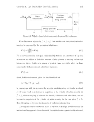
![Chapter 6. An Excavation Control Design 106
modelling observations, the compliant motion control methodology affords the ability
for greater flexibility in the system dynamics prescribed by the force compensator.
For example, consider the extension of equation (6.4) to include higher-order terms,
so that
H(s) = ms2
+ bs + k (6.6)
which leads to the force feedback law
vf = m
d2
dt2
fe + b
d
dt
fe + kfe . (6.7)
The parameters {m, b, k} would prescribe a desired dynamic response of the system
to varying intensities of bucket-rock interaction, as interpreted from dump cylinder
force measurements. Presumably, the particular admittance model selected would
impact the behaviour of the resulting control system when in contact with rock piles
of various composition. For example, the inclusion of the force damping term b might
improve the performance of the excavation controller in situations where large rock
fragments are present, adjusting the controller to respond appropriately by damping
out rapid changes in bucket-rock interaction intensity.
6.3.2 Modelling for Control System Simulation
In the compliant motion control literature, it is often the case that the environment
with which a robot manipulator interacts is modelled as a linear spring and damper
system; for example as in [40, 71, 89]. In many cases, this is sufficient and convenient
to describe the behaviour of simple environments. However, the process of bucket-
rock interaction discussed in this thesis is obviously a more complex system, and
therefore, its dynamics cannot be modelled by such convenient relationships, as was
noted by Hemami [32]. This issue becomes a problem when control system design
simulations are desired.](https://image.slidesharecdn.com/52609fa3-58a5-4f32-9c85-da30edc9900c-150416073852-conversion-gate02/85/Marshall-MScThesis-2001-122-320.jpg)
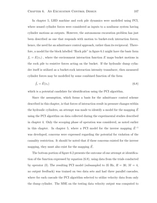
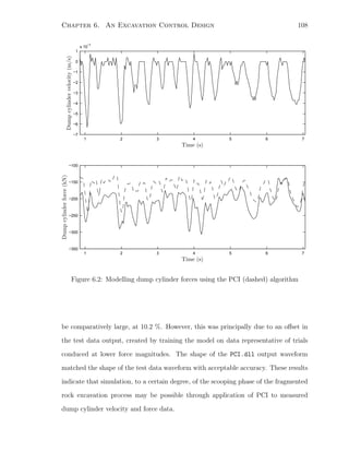
![Chapter 6. An Excavation Control Design 109
6.3.3 Further Remarks on the Excavation Control System
The control scheme proposed in this chapter forms the basis for an admittance con-
troller design towards autonomous excavation of fragmented rock. However, a number
of important details, necessary for implementation of the design, were not discussed.
Since controller implementation and tuning lies outside the scope of this dissertation,
only a qualitative examination of these issues is provided here.
Firstly, there remains the question of how to choose the proper force and velocity
setpoints fd and vd so as to achieve a full bucket of rock. Obviously, the values
assumed by these input arguments would depend heavily on the characteristics of the
excavation media. Intuitively, varying rock types and particle size distributions would
impact the optimal velocity and interaction intensity at which scooping should take
place. For instance, comparing the controlled excavation trials in the local roundstone
with those in the Inco muck discussed in chapter 4 (see figures 4.10 and 4.11 on pages
57 and 59), it is evident through observation of the breakout force that a higher
force setpoint would be desired for excavation in Inco rock (breakout at 260 kN) in
comparison with the local roundstone (breakout at 140 kN). Through inspection of
the aggressive excavation trial shown in figure 4.12 on page 60, one might select the
constant reference values fd ≈ 225 kN and vd ≈ 35 mm/s for excavation control. It
may be possible that suitable force and velocity setpoints be tuned, online, over a
series of excavation iterations, essentially adapting to potentially changing rock pile
characteristics.
Moreover, there remains the question of how to select an appropriate admittance
model Y (s), and model parameters, to be implemented by the force compensator.
This problem is compounded by the requirement that the given control system be
stable under varying excavation conditions. Seraji [89] noted that if the environment
impedance was known to change, possibly over several orders of magnitude, that a
fixed admittance design based on some nominal environment would often lead to](https://image.slidesharecdn.com/52609fa3-58a5-4f32-9c85-da30edc9900c-150416073852-conversion-gate02/85/Marshall-MScThesis-2001-125-320.jpg)
![Chapter 6. An Excavation Control Design 110
instability. It is reasonable to assume that, as the excavator bucket is passed through
any given rock pile, the impedance it sees as a result of bucket-rock interaction would
vary as the bucket is filled and particles of diverse sizes and shapes are encountered.
This issue was apparently dealt with by Seraji through the development of an adaptive
admittance technique for use in force control within a compliant motion framework.
It is worth noting that, with respect to a computed change in dump cylinder po-
sition xf (s) = 1
s
vf (s), the force compensator design of equation (6.6) is equivalent to
a proportional-integral-derivative (PID) regulator [89]. Rewriting the force feedback
law of equation (6.7) to compute the desired change in dump cylinder position yields
xf = m
d
dt
fe + bfe +
t
0
fedt (6.9)
where the parameters {m, b, k} become the derivative, proportional, and integral
gains, respectively. Although there exist techniques for tuning PID regulators [23,
page 191], it is likely that the necessary regulator gains depend not only on the
actuator and mechanism characteristics, but on the conditions and nature of each
excavation scenario.
Although control experiments and/or simulations were not performed, the admit-
tance control design proposed in this chapter, based on experimental and modelling
observations, and concepts from the field of compliant motion control, offers a first
look at one potential technique for control aimed specifically at the development of a
system for autonomous excavation of fragmented rock.](https://image.slidesharecdn.com/52609fa3-58a5-4f32-9c85-da30edc9900c-150416073852-conversion-gate02/85/Marshall-MScThesis-2001-126-320.jpg)
![Chapter 7
Summary and Conclusions
It is evident that undertaking the design of a system intended to perform autonomous
excavation of fragmented rock is a task that involves many unique and varied chal-
lenges. Most notably, the conditions necessary for a successful scooping operation are
seemingly influenced by the complex nature of bucket-rock interactions that occur
during excavation. In chapter 2, a relatively extensive review of the most pertinent
literature on this subject was presented, with a focus on those works relating most
specifically to the excavation of fragmented rock and to the automation of load-haul-
dump (LHD) mining machines. Despite the fact that an apparently broad range of
research has already been conducted in the field of autonomous excavation, none has
resulted in the prevalence of such technologies in the mining industry, nor in other
potentially relevant pursuits.
Previous studies in fragmented rock excavation were found to favour analytical
results, not validated through experimental means. For example, consider the ana-
lytical force analyses by Hemami [27, 29, 31, 32, 33] and the proposals for trajectory
generation by Mikhirev [61, 62]. Some researchers utilized laboratory-scale equipment
to validate approaches based on machine-vision [37, 73, 104] and behaviour-control
concepts [51, 52, 90]. Furthermore, it was discovered that the legitimacy of reviewed
111](https://image.slidesharecdn.com/52609fa3-58a5-4f32-9c85-da30edc9900c-150416073852-conversion-gate02/85/Marshall-MScThesis-2001-127-320.jpg)
![Chapter 7. Summary and Conclusions 112
empirical [21, 22, 61] and analytical [34, 101, 102, 105] studies in bucket-rock interac-
tion had yet to be confirmed by full-scale experimental studies aimed at identifying
a control system design suitable for autonomous excavation. Of the relevant patents
[15, 77], only one [15] was found to pertain specifically to excavation of fragmented
rock. Even so, it was not through a systems and control perspective that autonomous
excavation was claimed to have been achieved.
7.1 Experimental Excavation Studies
As a contribution to the task of filling a gap in the existing literature, a wide range of
full-scale experiments were conducted using a Tamrock EJC 9t model LHD machine,
under excavation conditions comparable to those found in an underground mining sit-
uation. The trial LHD machine was instrumented as was deemed appropriate in order
to measure certain operational dynamics during scooping. Machine parameters such
as hydraulic cylinder forces, loader mechanism configuration, and vehicle translation
were recorded, using instrumentation and data acquisition systems built specifically
for the described operations, with the intention of subsequent offline analyses and
system identification.
The excavation trials were conducted in two very different rock types: (i) a local
roundstone, and; (ii) a representative fragmented rock (Inco muck) taken from a
blast at an underground hard-rock mine and shipped to the testing site specifically
for the planned full-scale excavation trials. In addition to the recording of free-space
motion data, controlled and aggressive excavation experiments were conducted using
the aforementioned instrumentation and data acquisition systems.
For controlled excavation trials, observations were made regarding the status of
machine parameters during the penetration phase, scooping phase, and at breakout.
It was remarked that information contained within the dump cylinder force/motion](https://image.slidesharecdn.com/52609fa3-58a5-4f32-9c85-da30edc9900c-150416073852-conversion-gate02/85/Marshall-MScThesis-2001-128-320.jpg)
![Chapter 7. Summary and Conclusions 113
data was sufficient to expose a great deal about the excavation process. Aggressive
excavation trials were primarily intended to provide insight into the evolution of
machine parameters during successful scooping operations conducted by experienced
operators, and also to hint at potentially feasible approaches to automation of the
loading cycle. Hydraulic cylinder retraction rates, force/displacement changes, and
patterns in operator tactics were remarked.
7.2 Dynamics of the Loading Process
Having completed the full-scale experimental studies described above, the task of
developing a model capable of computing motions of the LHD loader mechanism
alone and while in contact with a given rock pile, was addressed. First, an analytical
approach for analysis of the LHD loader mechanism as a robot manipulator, using
techniques from Lagrangian mechanics, was outlined. Next, the employment of a dis-
tinct element method (DEM) and artificial neural networks were examined briefly as
modelling alternatives to the subsequently implemented parallel cascade identification
(PCI) algorithm.
It was reported recently by Eklund and Korenberg [19, 20] that the PCI algorithm
had been used to successfully identify aircraft pilot flight controls having a dynamic
model similar in mechanical nature to, although less complex than, the LHD loader
mechanism. Therefore, it was decided that an effort to employ the technique of PCI
to excavation modelling might be a worthwhile endeavour. Details were provided
regarding implementation of the PCI algorithm, for the purpose of validating its ap-
plicability to the given system identification problem. The developed C language
computer code was tested on contrived data to successfully prove its functionality
prior to modelling of systems represented by experimental data from full-scale ex-
cavation studies. PCI model identification scenarios pertaining to the LHD loader](https://image.slidesharecdn.com/52609fa3-58a5-4f32-9c85-da30edc9900c-150416073852-conversion-gate02/85/Marshall-MScThesis-2001-129-320.jpg)
![Chapter 7. Summary and Conclusions 114
mechanism forward dynamics in free-space and aggressive excavation trials were real-
ized. It was discovered that even the best outcomes were not exceptionally good, and
that this was particularly true when identifying dump cylinder motions in free-space.
However, it was also recognized that the mechanical system to be identified may have
depended heavily on its initial conditions, possibly explaining the less favourable re-
sults of attempts at modelling the more complicated dump cylinder dynamics. One
further point of contention was a possible violation of the causality assumption. The
presumption that bucket-rock interaction forces result in measurable cylinder pres-
sure changes formed a basis for the reactive control schemes of the reviewed patents
[77, 15] and the admittance control scheme proposed in chapter 6. Yet, the aggres-
sive excavation trial identification outcomes were sufficiently good to indicate that
violation of the causality restriction did not play a significant role.
7.3 Future Work in Excavation Control
In chapter 6, a thorough re-examination of the excavation control problem demon-
strated the potential applicability of concepts from the field of compliant motion
control to the task of autonomous excavation. A case for the formulation of a control
system design, founded on an approach labelled admittance control, was argued on the
basis of observations from full-scale experiments, modelling efforts, and conclusions
drawn in the reviewed literature and patent documents.
Contrary to a common notion that the environment must be an admittance and
the manipulator an impedance, a distinction was made that a solution to the problem
of autonomous excavation would be best achieved by a control system more closely
resembling pure force control. The admittance control approach, which dictates that
the manipulator accept force and respond with motion, is one that was found to
have not been explicitly explored in the literature pertaining to autonomous exca-](https://image.slidesharecdn.com/52609fa3-58a5-4f32-9c85-da30edc9900c-150416073852-conversion-gate02/85/Marshall-MScThesis-2001-130-320.jpg)
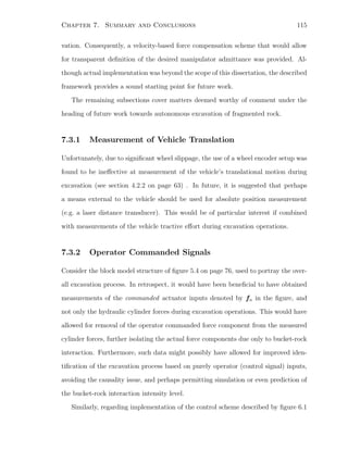
![Chapter 7. Summary and Conclusions 116
on page 105, and for identification, it would have been advantageous to have measured
operator commanded signals analogous to vc of the control system block diagram,
since the actual cylinder velocity vr is always corrupted to a certain degree by the
process of bucket-rock interaction. The extent to which bucket-rock interactions truly
influence excavator bucket motion could subsequently be determined. Other issues
that relate to this matter are discussed further in subsection 7.3.5.
7.3.3 On Tractive Effort
To reiterate previous statements regarding the issue of tractive effort (i.e. translational
force imparted to the rock pile by the wheels), an assumption was made that any
tractive effort supplied by the vehicle was generally constant throughout the loading
operation, and that tractive effort control would not have provided any significant
contribution to solving the autonomous excavation problem. This assumption was
weakly supported in the literature in that focus was given primarily to the problem
of determining appropriate bucket motions so as to achieve a full bucket of material.
For example, in the patent by Rocke et al. it was simply stated that, “. . . the operator
directs the machine to the pile of material, preferably at full throttle” [77].
Nonetheless, it is very much a possibility that measurement of the vehicle tractive
effort could provide further insight into the excavation process. Still, there exists a
significant challenge in physically measuring the level of tractive effort. Engine speed
would not be an effective measure, since the machine’s diesel engine is required in
most cases to power not only the wheels, but also the hydraulic pump that feeds the
actuating cylinders. If reaction forces at the boom link joint could be determined,
perhaps through strain gauge instrumentation, then it may also be possible to com-
pute an estimate of the tractive effort by considering it as a purely translational force
acting on the vehicle body. In any case, for the purposes of this thesis, the matters
surrounding tractive effort are afforded the status of future work.](https://image.slidesharecdn.com/52609fa3-58a5-4f32-9c85-da30edc9900c-150416073852-conversion-gate02/85/Marshall-MScThesis-2001-132-320.jpg)
![Chapter 7. Summary and Conclusions 117
7.3.4 Parallel Cascade Identification
Further to simply varying the model parameters, as was suggested in subsection
5.3.3 on page 89, there exist additional options for potential improvement of the PCI
modelling results of chapter 5. Firstly, it may be possible to enhance the results,
and perhaps identify more accurately situations where the cylinder was not moving
or capture abrupt changes in motion, by fitting a supplementary PCI model to the
error of the initial model [19, 20]. This second model could have a different memory
length and nonlinear degree than the original.
Also, in other research utilizing the PCI algorithm, it has been found that the
inclusion of a second dynamic linear element in each cascade (i.e. an LNL model)
has sometimes provided improved results [24, 46].
7.3.5 Simulation and Controller Development
There remains a great deal of research potential in the task of implementation and
application of the admittance control design proposed in chapter 6. Although it was
shown in subsection 6.3.2 on page 106 that simulation of the scooping phase of the
fragmented rock excavation process is perhaps possible through application of the
PCI algorithm, subsequent control simulations were not completed within the scope
of this thesis. As was stated in subsection 6.3.3 on page 109, implementation of the
admittance control design involves the resolution of issues such as: (i) extraction
of the PCI model parameters (not just the hi(j) and coefficients aim, but also the
normalizing coefficients discussed in subsection 5.3.1 on page 80); (ii) how to choose
the proper force and velocity setpoints fd and vd so as to achieve a full bucket of rock,
and; (iii) how to select an appropriate admittance model Y (s) to be implemented by
the force compensator H(s), which is effective and results in a stable system under
varying operational conditions.](https://image.slidesharecdn.com/52609fa3-58a5-4f32-9c85-da30edc9900c-150416073852-conversion-gate02/85/Marshall-MScThesis-2001-133-320.jpg)
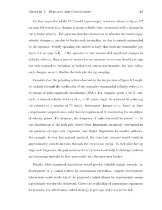
![Bibliography
[1] PX300, 302, 303 and 305 series pressure transducers. Omega Engineering, Inc.,
Stamford CT, U.S.A, 1996.
[2] Model H25 incremental optical encoder. BEI Technologies, Inc., Goleta CA,
U.S.A., November 1998.
[3] Presentation of the EJC 1000 prototype. Tamrock Loaders, Inc. Development
Engineering internal document, Burlington ON, Canada, March 1998.
[4] AMP04 precision single supply instrumentation amplifier, Rev. B. Analog De-
vices, Inc., Norwood MA, U.S.A., November 2000.
[5] Rayelco linear motion transducer. Ametek Aerospace, Gulton-Statham Prod-
ucts, Costa Mesa CA, U.S.A., 2000.
[6] S. Ashley. Underground mining from above. Mechanical Engineering, 117(5),
May 1995.
[7] J. Bares, P. C. Leger, P. Rowe, S. Singh, A. Stenz, and N. K. Lay. System
for autonomous excavation and truck loading. United Kingdom Patent No.
GB2342640, Carnegie Mellon University, April 2000.
[8] T. G. Beckwith, R. D. Marangoni, and J. H. Lienhard V. Mechanical Measure-
ments. Addison-Wesley Publishing Company, 5-th edition, 1993.
121](https://image.slidesharecdn.com/52609fa3-58a5-4f32-9c85-da30edc9900c-150416073852-conversion-gate02/85/Marshall-MScThesis-2001-137-320.jpg)
![Bibliography 122
[9] L. E. Bernold. Motion and path control for robotic excavation. Journal of
Aerospace Engineering, 6(1):1–18, January 1993.
[10] D. M. Bullock and I. J. Oppenheim. Object-oriented programming in robotics
research for excavation. Journal of Computing in Civil Engineering, 6(3):370–
385, July 1992.
[11] S. C. Chapra and R. P. Canale. Numerical Methods for Engineers. McGraw-Hill,
Inc., 2-nd edition, 1988.
[12] T-C. Chen. Linear System Theory and Design. Holt, Rinehard and Winston,
Inc., 1984.
[13] J. E. Colgate and N. Hogan. Robust control of dynamically interacting systems.
International Journal of Control, 48(1):65–88, 1988.
[14] P. A. Cundall and O. D. L. Strack. A discrete numerical model for granular
assemblies. G´eotechnique, 29(1):47–65, 1979.
[15] A. Dasys, L. Geoffroy, and A. Drouin. Sensor feedback control for automated
bucket loading. United States Patent No. 5941921, Noranda, Inc., August 1999.
[16] J. Denavit and R. S. Hartenberg. A kinematic notation for lower-pair mecha-
nisms based on matrices. Journal of Applied Mechanics, pages 215–221, June
1955.
[17] R. M. DeSantis. Modelling and path-tracking for a load-haul-dump mining vehi-
cle. ASME Journal of Dynamic Systems, Measurement and Control, 119:40–47,
1997.
[18] S. P. DiMaio, S. E. Salcudean, C. Reboulet, S. Tafazoli, and K. Hashtrudi-Zaad.
A virtual excavator for controller development and evaluation. In Proceedings](https://image.slidesharecdn.com/52609fa3-58a5-4f32-9c85-da30edc9900c-150416073852-conversion-gate02/85/Marshall-MScThesis-2001-138-320.jpg)
![Bibliography 123
of the 1998 IEEE International Conference on Robotics and Automation, vol-
ume 1, pages 52–58, 1998.
[19] J. M. Eklund. Aircraft flight control simulation using parallel cascade system
identification. M.Sc.(Eng.) thesis, Queen’s University, Kingston ON, Canada,
March 1998.
[20] J. M. Eklund and M. J. Korenberg. Simulation of aircraft pilot flight controls
using nonlinear system identification. Simulation, 75(2):72–81, 2000.
[21] Y. F. Fabrichnyi and S. B. Kolokolov. Calculating the resistance of blasted rock
to scooping by a bucket. Soviet Mining Science, 11(4):438–441, 1975.
[22] B. Forsman and C. L. Pan. Shear properties of fragmented rock masses: Model
tests and theories. International Journal of Rock Mechanics and Mining Science
Geomechanical Abstracts, 26(1):25–36, January 1989.
[23] G. F. Franklin, J. D. Powell, and A. Emami-Naeini. Feedback Control of Dy-
namic Systems. Addison-Wesley Publishing Company, Inc., 3-rd edition, 1994.
[24] A. S. French, M. J. Korenberg, M. Jarvilehto, E. Kouvalainen, M. Juusola, and
M. Weckstrom. The dynamic nonlinear behavior of fly photoreceptors evoked
by a wide range of light intensities. Biophysical Journal, 65:832–839, 1993.
[25] F. H. Ghorbel, O. Ch´etelat, R. Gunawardana, and R. Longchamp. Modeling
and set point control of closed-chain mechanism: Theory and experiment. IEEE
Transactions on Control Systems Technology, 8(5):801–815, September 2000.
[26] Q. P. Ha, Q. H. Nguyen, D. C. Rye, and H. F. Durrant-Whyte. Impedance con-
trol of a hydraulically actuated robotic excavator. Automation in Construction,
9(5):421–435, 2000.](https://image.slidesharecdn.com/52609fa3-58a5-4f32-9c85-da30edc9900c-150416073852-conversion-gate02/85/Marshall-MScThesis-2001-139-320.jpg)
![Bibliography 124
[27] A. Hemami. A conceptual approach to automation of LHD-loaders. In Pro-
ceedings of the Canadian Symposium on Mining Automation, pages 178–183,
September 1992.
[28] A. Hemami. Force analysis in the scooping/loading operation of an LHD loader.
In Proceedings of the 2nd International Symposium on Mine Mechanization and
Automation, pages 415–424, 1993.
[29] A. Hemami. Study of bucket trajectory in automatic scooping with load-haul-
dump loaders. In Transactions of the Institution of Mining and Metallurgy,
Series A: Mining Industry, volume 102, pages A37–A42, January–April 1993.
[30] A. Hemami. An approximation of the weight of the loaded material during
the scooping operation of a mechanical loader. Transactions of the Canadian
Society for Mechanical Engineering, 18(3):191–205, 1994.
[31] A. Hemami. Modelling, analysis and preliminary studies for automatic scooping.
Advanced Robotics, 8(5):511–529, 1994.
[32] A. Hemami. Fundamental analysis of automatic excavation. Journal of
Aerospace Engineering, 8(4):175–179, October 1995.
[33] A. Hemami and L. K. Daneshmend. Force analysis for automation of the loading
operation in an LHD-loader. In Proceedings of the 1992 IEEE International
Conference on Robotics and Automation, pages 645–650, 1992.
[34] A. Hemami, S. Goulet, and M. Aubertin. Resistance of particulate media to
excavation: Application to bucket loading. International Journal of Surface
Mining, Reclamation and Environment, 8:125–129, 1994.](https://image.slidesharecdn.com/52609fa3-58a5-4f32-9c85-da30edc9900c-150416073852-conversion-gate02/85/Marshall-MScThesis-2001-140-320.jpg)
![Bibliography 125
[35] A. Hemami and V. Polotski. Path tracking control problem formulation of an
LHD loader. The International Journal of Robotics Research, 17(2):193–199,
1998.
[36] N. Hogan. Impedance control: An approach to manipulation, Parts I, II, and
III. ASME Journal of Dynamic Systems, Measurement, and Control, 107:1–24,
1985.
[37] Q. Ji and R. L. Sanford. Autonomous excavation of fragmented rock using
machine vision. In Emerging Computer Techniques for the Minerals Industry,
chapter 24, pages 221–228. Society for Mining, Metallurgy Exploration Inc.,
Littleton CO, U.S.A., 1993.
[38] P. D. Katsabanis. Fragmentation, vibrations, blast design. MINE321 course
notes, Queen’s University, Kingston ON, Canada, 1998.
[39] H. Kazerooni, T. B. Sheridan, and P. K. Houpt. Robust compliant motion
for manipulators, Parts I and II. IEEE Journal of Robotics and Automation,
RA-2(2):83–105, June 1986.
[40] H. Kazerooni, B. J. Waibel, and S. Kim. On the stability of robot compliant
motion control: Thoery and experiments. ASME Journal of Dynamic Systems,
Measurement, and Control, 112:417–426, 1990.
[41] A. J. Koivo, M. Thoma, E. Kocaoglan, and J. Andrade-Cetto. Modeling and
control of excavator dynamics during digging operation. Journal of Aerospace
Engineering, 9(1):10–18, January 1996.
[42] M. J. Korenberg. Identifying nonlinear difference equation and functional ex-
pansion representations: The fast orthogonal algorithm. Annals of Biomedical
Engineering, 16:123–142, 1988.](https://image.slidesharecdn.com/52609fa3-58a5-4f32-9c85-da30edc9900c-150416073852-conversion-gate02/85/Marshall-MScThesis-2001-141-320.jpg)
![Bibliography 126
[43] M. J. Korenberg. A robust orthogonal algorithm for system identification and
time-series analysis. Biological Cybernetics, 60:267–276, 1989.
[44] M. J. Korenberg. Parallel cascade identification and kernal estimation for non-
linear systems. Annals of Biomedical Engineering, 19:429–455, 1991.
[45] M. J. Korenberg. Personal communications, June 2001.
[46] M. J. Korenberg. Personal communications, July 2001.
[47] M. J. Korenberg, S. B. Bruder, and P. J. McIlroy. Exact orthogonal kernel esti-
mation from finite data records: Extending Wiener’s identification of nonlinear
systems. Annals of Biomedical Engineering, 16:201–214, 1988.
[48] D. Kumar and N. Vagenas. Performance evaluation of an automatic load-haul-
dump vehicle. CIM Bulletin, 86(974):39–42, 1993.
[49] Y. Laperri`ere and F. Miller. Automatic loading of LHDs. In Proceedings of
Telemin 1 and the 5th International Symposium on Mine Mechanization and
Automation, June 1999.
[50] A. T. Le, Q. Nguyen, Q. P. Ha, D. Rye, H. Durrant-Whyte, M. Stevens, and
V. Boget. Towards autonomous excavation. In Proceedings of the International
Conference on Field and Service Robotics, pages 121–126. Australian Robot
Association, 1997.
[51] P. J. A. Lever and F-Y. Wang. Intelligent excavator control system for lunar
mining system. Journal of Aerospace Engineering, 8(1):16–24, January 1995.
[52] P. J. A. Lever, F-Y. Wang, and X. Shi. Using bucket force/torque feedback for
control of an automated excavator. In Transactions, volume 300, pages 135–139.
Society for Mining, Metallurgy Exploration, 1996.](https://image.slidesharecdn.com/52609fa3-58a5-4f32-9c85-da30edc9900c-150416073852-conversion-gate02/85/Marshall-MScThesis-2001-142-320.jpg)
![Bibliography 127
[53] A. D. Lewis. Lagrangian mechanics, dynamics, and control. MATH439 course
notes, Queen’s University, Kingston ON, Canada, January 2001.
[54] W. Lidkea. Personal communications, June 2001.
[55] S-K. Lin. Dynamics of the manipulator with closed chains. IEEE Transactions
on Robotics and Automation, 6(4):496–501, August 1990.
[56] J. Y. S. Luh and Y-F. Zheng. Computation of input generalized forces for
robots with closed kinematic chain mechanisms. IEEE Journal of Robotics and
Automation, RA-1(2):95–103, June 1985.
[57] R. Madhavan, M. W. M. G. Dissanayake, and H. F. Durrant-Whyte. Au-
tonomous underground navigation of an LHD using a combined ICP-EKF ap-
proach. In Proceedings of the 1998 IEEE International Conference on Robotics
and Automation, volume 4, pages 3703–3708, 1998.
[58] The MathWorks, Inc., Natick MA, U.S.A. Application Program Interface Guide,
Version 5, 1998.
[59] P. J. H. McIlroy. Applications of nonlinear systems identification. M.Sc. thesis,
Queen’s University, Kingston ON, Canada, 1984.
[60] K. Mehrotra, C. K. Mohan, and S. Ranka. Elements of Artificial Neural Net-
works. Series in Complex Adaptive Systems. Massachusetts Institute of Tech-
nology Press, 1997.
[61] P. A. Mikhirev. Theory of the working cycle of automated rock-loading machines
of periodic action. Soviet Mining Science, 19(6):515–522, 1983.
[62] P. A. Mikhirev. Design of automated loading buckets. Soviet Mining Science,
22(4):292–298, 1986.](https://image.slidesharecdn.com/52609fa3-58a5-4f32-9c85-da30edc9900c-150416073852-conversion-gate02/85/Marshall-MScThesis-2001-143-320.jpg)
![Bibliography 128
[63] P. Murphy. Personal communications, November 2000.
[64] P. Murphy. Load-haul-dump vehicle load history data acquisition and analysis.
M.Sc.(Eng.) thesis, Queen’s University, Kingston ON, Canada, September 2001.
Pending submission and acceptance.
[65] J. J. Murray and G. H. Lovell. Dynamic modeling of closed-chain robotic
manipulators and implications for trajectory control. IEEE Transactions on
Robotics and Automation, 5(4):522–528, August 1989.
[66] Y. Nakamura and M. Ghodoussi. Dynamics computation of closed-link robot
mechanisms with nonredundant and redundant actuators. IEEE Transactions
on Robotics and Automation, 5(3):294–302, June 1989.
[67] National Instruments Corporation, Austin TX, U.S.A. DAQ: SCC Series User
Manual, December 1999.
[68] National Instruments Corporation, Austin TX, U.S.A. National Instruments
LabVIEW Measurements Manual, July 2000.
[69] National Instruments Corporation, Austin TX, U.S.A. National Instruments
LabVIEW Users Manual, July 2000.
[70] W. S. Newman. Stability and performance limits of interaction controllers.
ASME Journal of Dynamic Systems, Measurement, and Control, 114:563–570,
December 1992.
[71] M. Pelletier and L. K. Daneshmend. Automatic synthesis of robot compliant
motions in dynamic environments. International Journal of Robotics Research,
16(6):730–748, 1997.
[72] M. Pelletier and M. Doyon. On the implementation and performance of
impedance control on position controlled robots. In Proceedings of the 1994](https://image.slidesharecdn.com/52609fa3-58a5-4f32-9c85-da30edc9900c-150416073852-conversion-gate02/85/Marshall-MScThesis-2001-144-320.jpg)
![Bibliography 129
IEEE International Conference on Robotics and Automation, volume 2, pages
1228–1233, 1994.
[73] M. K. Petty, J. Billingsley, and T. Tran-Cong. Autonomous LHD loading.
In Proceedings of the Annual IEEE Conference on Mechatronics and Machine
Vision in Practice, pages 219–224, 1997.
[74] M. Piotte, C. Coache, A. Drouin, P. Gauthier, and L. Geoffroy. Automatic
control of underground vehicles at high speed. CIM Bulletin, 90(1003):78–81,
1997.
[75] M. Raibert and J. J. Craig. Hybrid position/force control of manipulators.
ASME Journal of Dynamic Systems, Measurement, and Control, June 1981.
[76] D. J. Rocke. Automatic excavation control system and method. United States
Patent No. 5446980, Caterpillar Inc., September 1995.
[77] D. J. Rocke. Control system for automatically controlling a work implement
of an earthworking machine to capture material. United States Patent No.
5528843, Caterpillar Inc., June 1996.
[78] D. J. Rocke. Self-adapting excavation control system and method. United
States Patent No. 5682312, Caterpillar Inc., October 1997.
[79] G. V. Rodionov. Theory of the working cycle of rock loaders of a periodic
action. Transactions of the Mining and Geological Institute, 19, 1957. Academy
of Sciences of the USSR, Ural Branch (in Russian).
[80] G. J. S. Ross. Nonlinear Estimation. Springer Series in Statistics. Springer-
Verlag New York, Inc., 1990.](https://image.slidesharecdn.com/52609fa3-58a5-4f32-9c85-da30edc9900c-150416073852-conversion-gate02/85/Marshall-MScThesis-2001-145-320.jpg)
![Bibliography 130
[81] P. S. Rowe. Learning system and method for optimizing control of autonomous
earthmoving machinery. United States Patent No. 6076030, Carnegie Mellon
University, June 2000.
[82] W. J. Rugh. Nonlinear System Theory: The Volterra/Wiener Approach. The
Johns Hopkins University Press, 1981.
[83] D. E. Rumelhart, G. E. Hinton, and R. J. Williams. Learning internal repre-
sentations by error propagation. Parallel Distributed Processing, 1, 1986.
[84] S. E. Salcudean, K. Hashtrudi-Zaad, S. Tafazoli, S. P. DiMaio, and C. Reboulet.
Bilateral matched impedance teleoperation with application to excavator con-
trol. In Proceedings of the 1998 IEEE International Conference on Robotics and
Automation, pages 133–139, May 1998.
[85] S. E. Salcudean, S. Tafazoli, P. D. Lawrence, and I. Chau. Impedance control
of a teleoperated mini excavator. In Proceedings of the 8th IEEE International
Conference on Advanced Robotics (ICAR), July 1997.
[86] S. Sarata, K. Sata, and S. Tsukuba. Motion control system for autonomous
wheel loader operation. In Proceedings of the 1998 International Conference on
Mine Mechanization and Automation, pages 13.1–13.12, 1998.
[87] D. Sargent. Personal communications, October 2000.
[88] M. Schetzen. The Volterra and Wiener Theories of Nonlinear Systems. John
Wiley Sons, Inc., 1980.
[89] H. Seraji. Adaptive admittance control: An approach to explicit force control
in compliant motion. In Proceedings of the 1994 IEEE International Conference
on Robotics and Automation, pages 2705–2712, 1994.](https://image.slidesharecdn.com/52609fa3-58a5-4f32-9c85-da30edc9900c-150416073852-conversion-gate02/85/Marshall-MScThesis-2001-146-320.jpg)
![Bibliography 131
[90] X. Shi, P. J. A. Lever, and F-Y. Wang. Experimental robotic excavation with
fuzzy logic and neural networks. In Proceedings of the 1996 IEEE International
Conference on Robotics and Automation, volume 1, pages 957–962, April 1996.
[91] X. Shi, P. J. A. Lever, and F-Y. Wang. Autonomous Rock Excavation: Intelli-
gent Control Techniques and Experimentation, volume 10 of Series in Intelligent
Control and Intelligent Automation. World Scientific Publishing Co. Pte. Ltd.,
1998.
[92] T. Shinji. Automatic excavation system of loading machine. Japanese Patent
No. JP62291335, Komatsu Ltd., December 1987.
[93] T. Shinji. Method and apparatus for automatic excavation of loading machine.
Japanese Patent No. JP62185928, Komatsu Ltd., August 1987.
[94] T. Shoji and O. Tomoaki. Automatic control device for hydraulic shovel.
Japanese Patent Office Publication No. 09256407, Shin Caterpillar Mitsubishi
Ltd., September 1997.
[95] S. Singh. Learning to predict resistive forces during robotic excavation. In
Proceedings of the 1995 IEEE International Conference on Robotics and Au-
tomation, volume 2, pages 2102–2107, 1995.
[96] N. K. Sinha and B. Kuszta. Modeling and Identification of Dynamic Systems.
Van Nostrand Reinhold Electrical/Computer Science and Engineering Series.
Van Nostrand Reinhold Company, 1983.
[97] M. R. Spiegel. Theory and Problems of Theoretical Mechanics. McGraw-Hill,
Inc., 1967.
[98] M. W. Spong and M. Vidyasagar. Robot Dynamics and Control. John Wiley
Sons, Inc., 1989.](https://image.slidesharecdn.com/52609fa3-58a5-4f32-9c85-da30edc9900c-150416073852-conversion-gate02/85/Marshall-MScThesis-2001-147-320.jpg)
![Bibliography 132
[99] J. Steele, C. Ganesh, and A. Kleve. Control and scale model simulation of
sensor-guided LHD mining machines. IEEE Transactions on Industry Applica-
tions, 29(6):1232–1238, 1993.
[100] A. Stentz, J. Bares, S. Singh, and P. Rowe. A robotic excavator for autonomous
truck loading. Autonomous Robots, 7(2):175–186, 1999.
[101] H. Takahashi. Simulation of the resistive forces acting on the bucket of wheel
loader in the robotic scooping by use of DEM. In Proceedings of the Inter-
national Association of Science and Technology for Development (IASTED)
Conference: Robotics and Automation 2000, pages 230–235, August 2000.
[102] H. Takahashi, M. Hasegawa, and E. Nakano. Analysis on the resistive forces
acting on the bucket of a load-haul-dump machine and a wheel loader in the
scooping task. Advanced Robotics, 13(2):97–114, 1999.
[103] H. Takahashi, H. Kamata, T. Masuyama, and S. Sarata. Concept and model
experiments on automatic shoveling of rocks from the rock piles. Computers
Industrial Engineering, 27(1–4):43–46, 1994.
[104] H. Takahashi, H. Kamata, T. Masuyama, and S. Sarata. Autonomous shoveling
of rocks by using image vision system on LHD. In Proceedings of the 1998
International Conference on Mine Mechanization and Automation, pages 1.33–
1.44, 1998.
[105] H. Takahashi, Y. Tsukamoto, and E. Nakano. Analysis of resistive forces acting
on the bucket of LHD in the scooping task. In Proceedings of the 16th Interna-
tional Symposium on Automation and Robotics in Construction, pages 517–522,
1999.
[106] P. K. V¨ah¨a and M. J. Skibniewski. Cognitive force control of excavators. Journal
of Aerospace Engineering, 6(2):159–166, April 1993.](https://image.slidesharecdn.com/52609fa3-58a5-4f32-9c85-da30edc9900c-150416073852-conversion-gate02/85/Marshall-MScThesis-2001-148-320.jpg)
![Bibliography 133
[107] D. A. Wells. Theory and Problems of Lagrangian Dynamics. McGraw-Hill, Inc.,
1967.
[108] D. E. Whitney. Force feedback control of manipulator fine motions. ASME
Journal of Dynamic Systems, Measurement, and Control, pages 91–97, June
1977.](https://image.slidesharecdn.com/52609fa3-58a5-4f32-9c85-da30edc9900c-150416073852-conversion-gate02/85/Marshall-MScThesis-2001-149-320.jpg)
![Appendix A
Hardware Specifications
This appendix presents specification data that was not included in the text of chapters
4 and 5. The following tables offer only immediately relevant summary information.
For full hardware specification details, refer to the cited references for each table.
A.1 Loader Specifications
Table A.1: General specifications for the Tamrock EJC 9t LHD machine [3]
Carrying capacity 22,000 lbs 10 000 kg
Bucket size 6.0 yd3
4.6 m3
Engine power 247 hp 182 kW
Table A.2: Hydraulic cylinder general specifications [3]
Lift cylinder(s) — Dump cylinder —
Bore diameter 7 in 180 mm 8 in 200 mm
Rod diameter 3.5 in 90 mm 4 in 110 mm
Stroke length 43 in 1100 mm 100 in 2510 mm
134](https://image.slidesharecdn.com/52609fa3-58a5-4f32-9c85-da30edc9900c-150416073852-conversion-gate02/85/Marshall-MScThesis-2001-150-320.jpg)
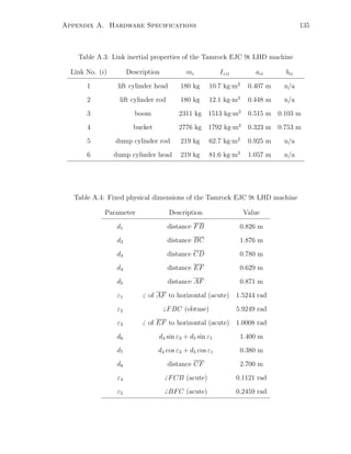
![Appendix A. Hardware Specifications 136
A.2 Sensor Specifications
Table A.5: PX303 series pressure transducer specifications [1]
Excitation 12–32 V (dc)
Output 0.5–5.5 V (dc)
Accuracy 0.25% F.S.
Minimum Load Resistance 2000 Ω
Response Time 1 ms
Table A.6: P-60A linear motion transducer specifications [5]
Excitation 5.00 V (dc)
Linearity 0.08% F.S.
Potentiometer Resistance 500 Ω
Stroke 60.00 in
Table A.7: Specifications for the model H25 incremental optical encoder [2]
Supply voltage 5–15 V (dc), vin = vout
Output format 2 channels in quadrature
Frequency response 100 kHz
Cycles per shaft turn 1000
Maximum speed 12 000 rpm
Shaft diameter 3/8 in (nominal)](https://image.slidesharecdn.com/52609fa3-58a5-4f32-9c85-da30edc9900c-150416073852-conversion-gate02/85/Marshall-MScThesis-2001-152-320.jpg)
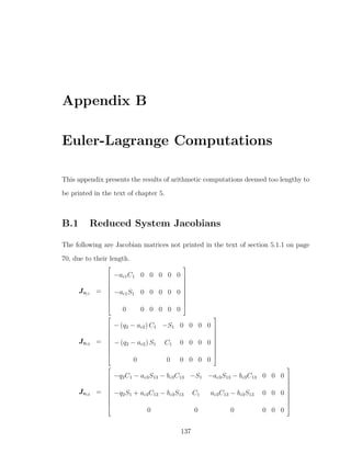
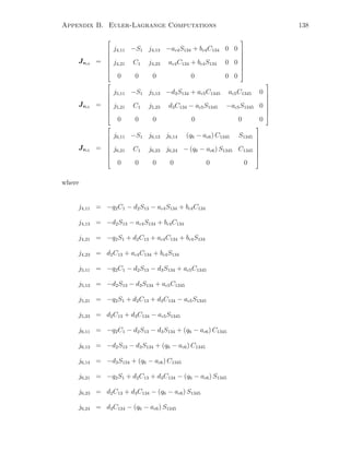


![JOB PORTFOLIO_PRASHANTH_2015 [Compatibility Mode]](https://cdn.slidesharecdn.com/ss_thumbnails/cfe82d46-004b-4f25-be17-1f46c5ab1afc-150923190817-lva1-app6891-thumbnail.jpg?width=640&height=640&fit=bounds)


