Download to read offline

![LIST OF FIGURES
2.1 The original image with 6 grayscale values (a) and its histogram (b). The re-
duced image with 3 grayscale values (c) and its histogram (d). . . . . . . . . . 7
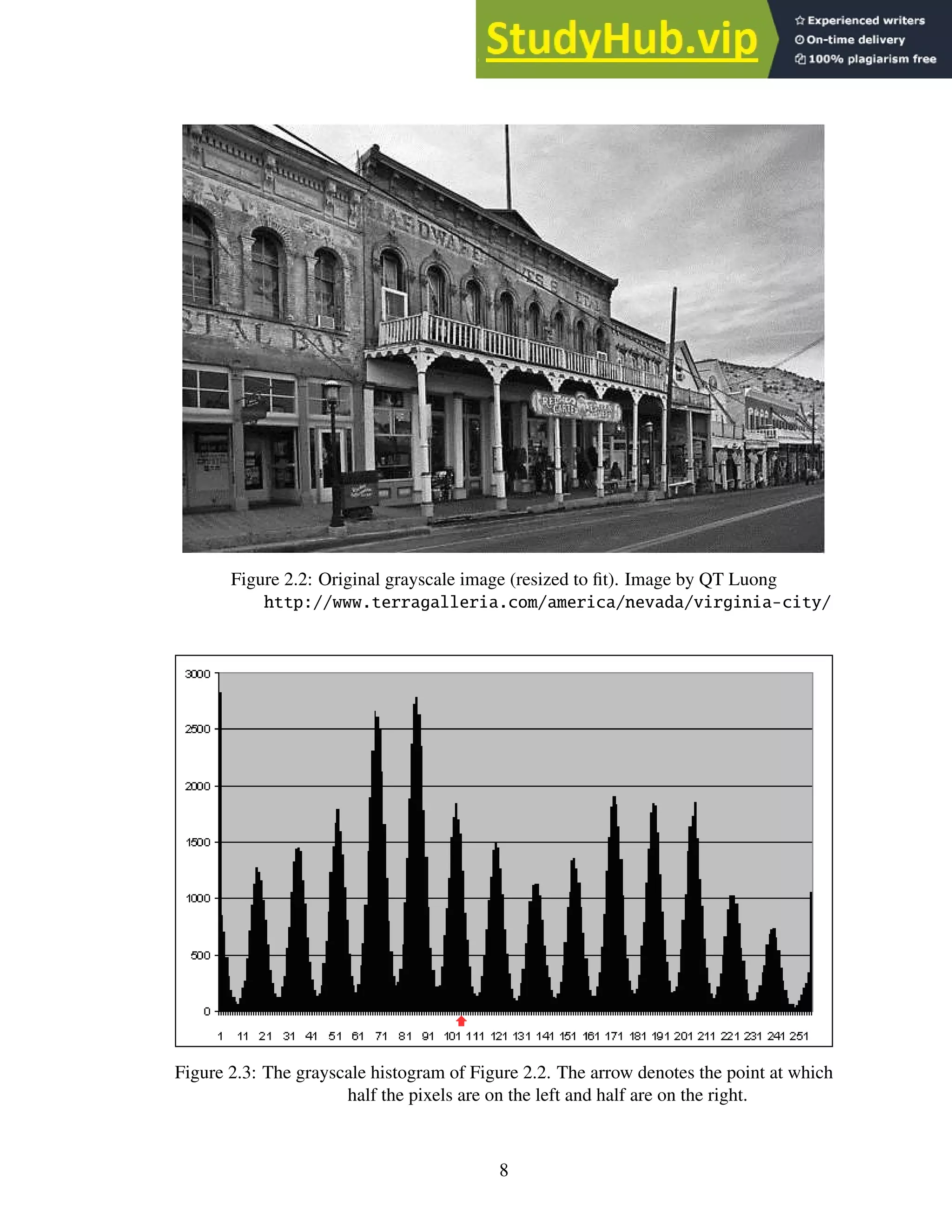
2.2 Original grayscale image (resized to fit). Image by QT Luong http://www.
terragalleria.com/america/nevada/virginia-city/ . . . . . . . . . . 8
2.3 The grayscale histogram of Figure 2.2. The arrow denotes the point at which
half the pixels are on the left and half are on the right. . . . . . . . . . . . . . . 8
2.4 Original image after the threshold from Figure 2.3 is applied. . . . . . . . . . . 9
2.5 (a) and (c) show the two chain code scoring methods; (b) and (d) show a sam-
ple chain using their respective scoring methods; (e) shows an ‘a’ and its cor-
responding chain code. The arrow denotes the starting position for each chain
code. . . . . . . . . . . . . . . . . . . . . . . . . . . . . . . . . . . . . . . . . 10
2.6 Horizontal and vertical projection profiles. Figure recreated from Abdelwahab
et al. [56]. . . . . . . . . . . . . . . . . . . . . . . . . . . . . . . . . . . . . . 11
2.7 Nearest-neighbor clustering uses the angle between pixel groups to compute
rotation. In this example, the glyphs themselves form the pixel groups. . . . . . 12
2.8 Depiction of the mean line and base line. Figure recreated from Das et al. [12]. 12
2.9 The Hough transform projects lines through pixels and counts the intersections
to find the mean line and the baseline. . . . . . . . . . . . . . . . . . . . . . . 13
2.10 An example 2×2-pixel morphological close operation. (a) the original shape,
(b) the shape after the structuring element is applied. . . . . . . . . . . . . . . 13
2.11 An example 2×2-pixel morphological open operation. (a) the original shape,
(b) the shape after the structuring element is applied. . . . . . . . . . . . . . . 14
2.12 The Das and Chanda morphology method. (a) the original text, (b) the text
after the close operation using a 12 pixel horizontal structuring element. (c)
the text after the open operation with a 5 pixel x 5 pixel structuring element.
(d) the transitions from black to white pixels, representing the baseline of the
text. . . . . . . . . . . . . . . . . . . . . . . . . . . . . . . . . . . . . . . . . 14
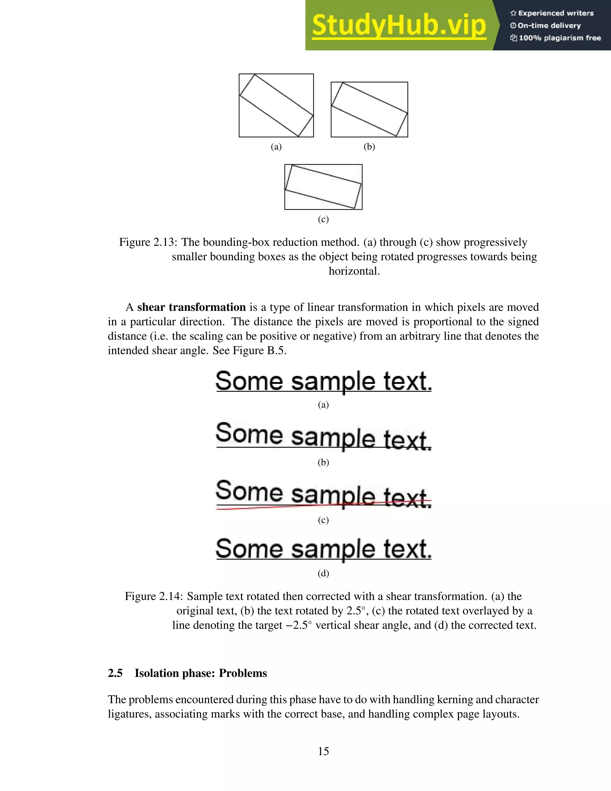
2.13 The bounding-box reduction method. (a) through (c) show progressively smaller
bounding boxes as the object being rotated progresses towards being horizontal. 15
2.14 Sample text rotated then corrected with a shear transformation. (a) the original
text, (b) the text rotated by 2.5◦
, (c) the rotated text overlayed by a line denoting
the target −2.5◦
vertical shear angle, and (d) the corrected text. . . . . . . . . . 15
2.15 Chain codes can isolate kerned characters like those in (a). The chain code in
(c) represents the outside edge of the ’J’ character in (b). . . . . . . . . . . . . 17
2.16 Borders for a best-fit bounding box. . . . . . . . . . . . . . . . . . . . . . . . 17
2.17 The execution of the path-finding algorithm to find the white space between
characters. . . . . . . . . . . . . . . . . . . . . . . . . . . . . . . . . . . . . . 17
2.18 PathFind pseudo code. . . . . . . . . . . . . . . . . . . . . . . . . . . . . . . 19
2.19 Possible vertical boundary borders of a best-fit bounding box. . . . . . . . . . . 20
vi](https://image.slidesharecdn.com/anopticalcharacterrecognitionengineforgraphicalprocessingunits-230805215723-24ac1bd2/75/An-Optical-Character-Recognition-Engine-For-Graphical-Processing-Units-9-2048.jpg)
![2.20 Several potential chop points that the Tesseract OCR engine might use to over-
come ligatures. Figure recreated from Smith [53]. . . . . . . . . . . . . . . . . 20
2.21 A complex page layout with horizontal and vertical projection graphs. Valleys
in the graphs show potential split points. . . . . . . . . . . . . . . . . . . . . . 21
2.22 (a) the original paragraph, (b) and (c) horizontal and vertical smearing, respec-
tively, using a 6 pixel threshold. . . . . . . . . . . . . . . . . . . . . . . . . . . 22
2.23 White-space analysis finds set of rectangles that comprise white space within
the document. The gray rectangles indicate white space. . . . . . . . . . . . . . 22
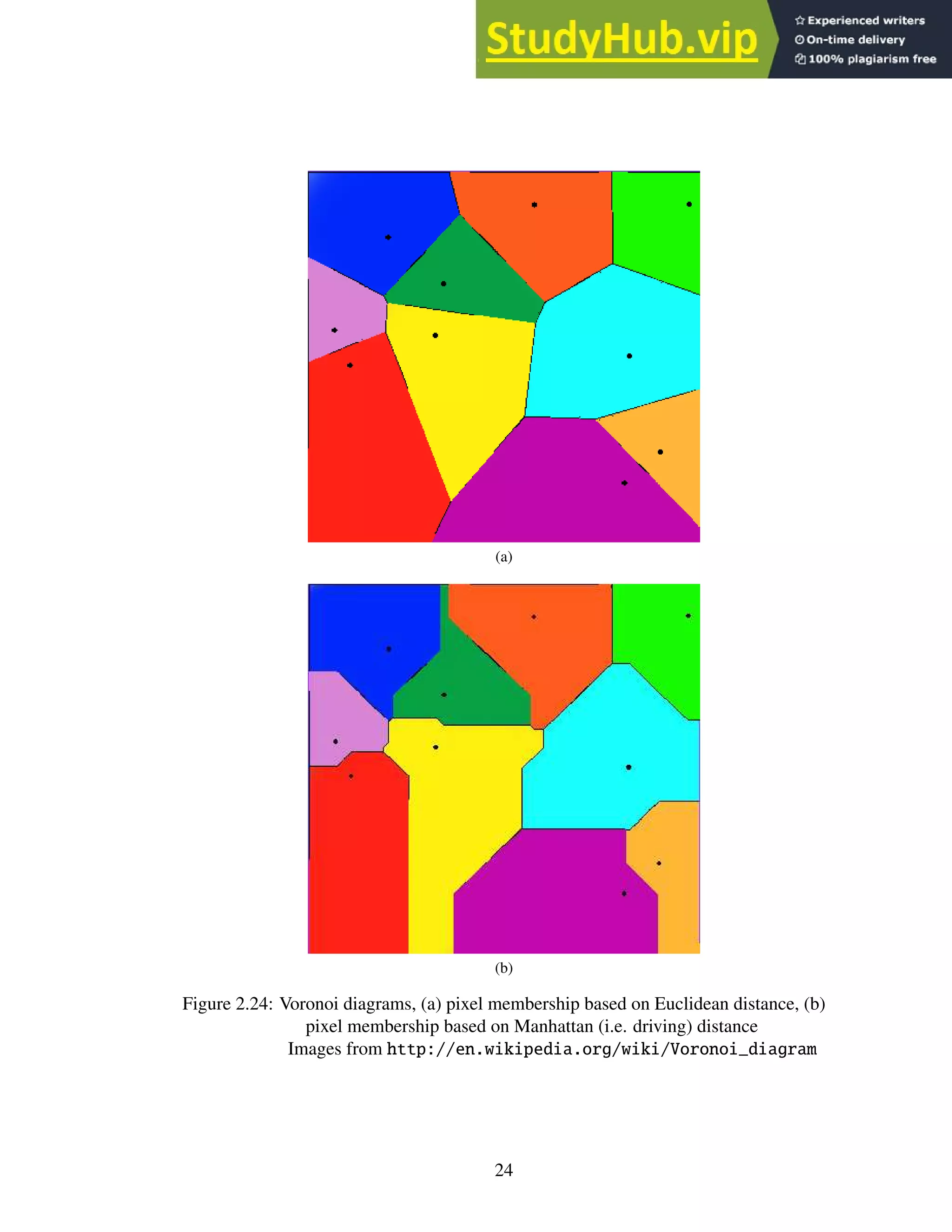
2.24 Voronoi diagrams, (a) pixel membership based on Euclidean distance, (b) pixel
membership based on Manhattan (i.e. driving) distance
Images from http://en.wikipedia.org/wiki/Voronoi_diagram . . . . . 24
2.25 Multiple color image with negative color text and isolated color components,
(a) the original image, (b) the R component, (c) the G component, (d) the B
component. . . . . . . . . . . . . . . . . . . . . . . . . . . . . . . . . . . . . 25
2.26 The letter ‘A’ undergoing horizontal skeletonization. The gray pixels indicate
pixels selected for deletion. . . . . . . . . . . . . . . . . . . . . . . . . . . . . 27
2.27 (a) the original character (b) horizontal runs (c) runs marked as splitting or
merging; unmarked runs are continuous (d) blocks (e) centroid computation (f)
connected centroids. Figure recreated from Lakshmi et al. [26]. . . . . . . . . . 28
2.28 Allowed connection paths. The sizes are not relative. Figure recreated from
Lakshmi et al. [26]. . . . . . . . . . . . . . . . . . . . . . . . . . . . . . . . . 28
2.29 The calculated skeleton. . . . . . . . . . . . . . . . . . . . . . . . . . . . . . . 28
2.30 (a) a 72pt character scaled down to 36pt. (b) a 12pt character scaled up to 36pt.
(c) an original 36pt character. . . . . . . . . . . . . . . . . . . . . . . . . . . . 28
2.31 The black and white dots show the sampling positions. (a) the original charac-
ters with various orientations within the image. (b) the resultant scaled-down
characters. Figure recreated from Barrera et al. [6]. . . . . . . . . . . . . . . . 29
2.32 (a) the original degraded characters; (b) the combined “stamp”. . . . . . . . . . 30
2.33 (a) the original character (b) a set of shape priors (c) – (g) shape prior border
alignment; the arrow depicts the most likely border for alignment. The image
degradation is intentional. . . . . . . . . . . . . . . . . . . . . . . . . . . . . . 31
2.34 (a) shape priors and (b) the confidence map. Darker pixels are more likely
to appear and are weighted more heavily during comparisons with unknown
characters. . . . . . . . . . . . . . . . . . . . . . . . . . . . . . . . . . . . . . 31
2.35 A character glyph segmented into 3×3 pixel segments. . . . . . . . . . . . . . 32
2.36 (a) vertical longest run (b) horizontal longest run (c) vertical and horizontal
pixel intersections through the center of the bounding box. . . . . . . . . . . . 33
2.37 (a) the pattern and legend (b) original character (c) the pattern applied across
the original character image at three of the many possible positions. . . . . . . 33
2.38 (a) three 72pt Arial characters overlayed on one another (b) filled locations are
unique to a single character. . . . . . . . . . . . . . . . . . . . . . . . . . . . . 34
2.39 Fourier transform of sinusoidal brightness images. . . . . . . . . . . . . . . . . 35
2.40 Fourier transform of 3 character images. . . . . . . . . . . . . . . . . . . . . . 36
2.41 Several examples of wavelet basis functions.
Images from http://en.wikipedia.org/wiki/Wavelet . . . . . . . . . . 37
vii](https://image.slidesharecdn.com/anopticalcharacterrecognitionengineforgraphicalprocessingunits-230805215723-24ac1bd2/75/An-Optical-Character-Recognition-Engine-For-Graphical-Processing-Units-10-2048.jpg)
![2.42 The Haar wavelet.
Image from http://en.wikipedia.org/wiki/Haar_wavelet . . . . . . . 38
2.43 The Haar transform in action. . . . . . . . . . . . . . . . . . . . . . . . . . . . 39
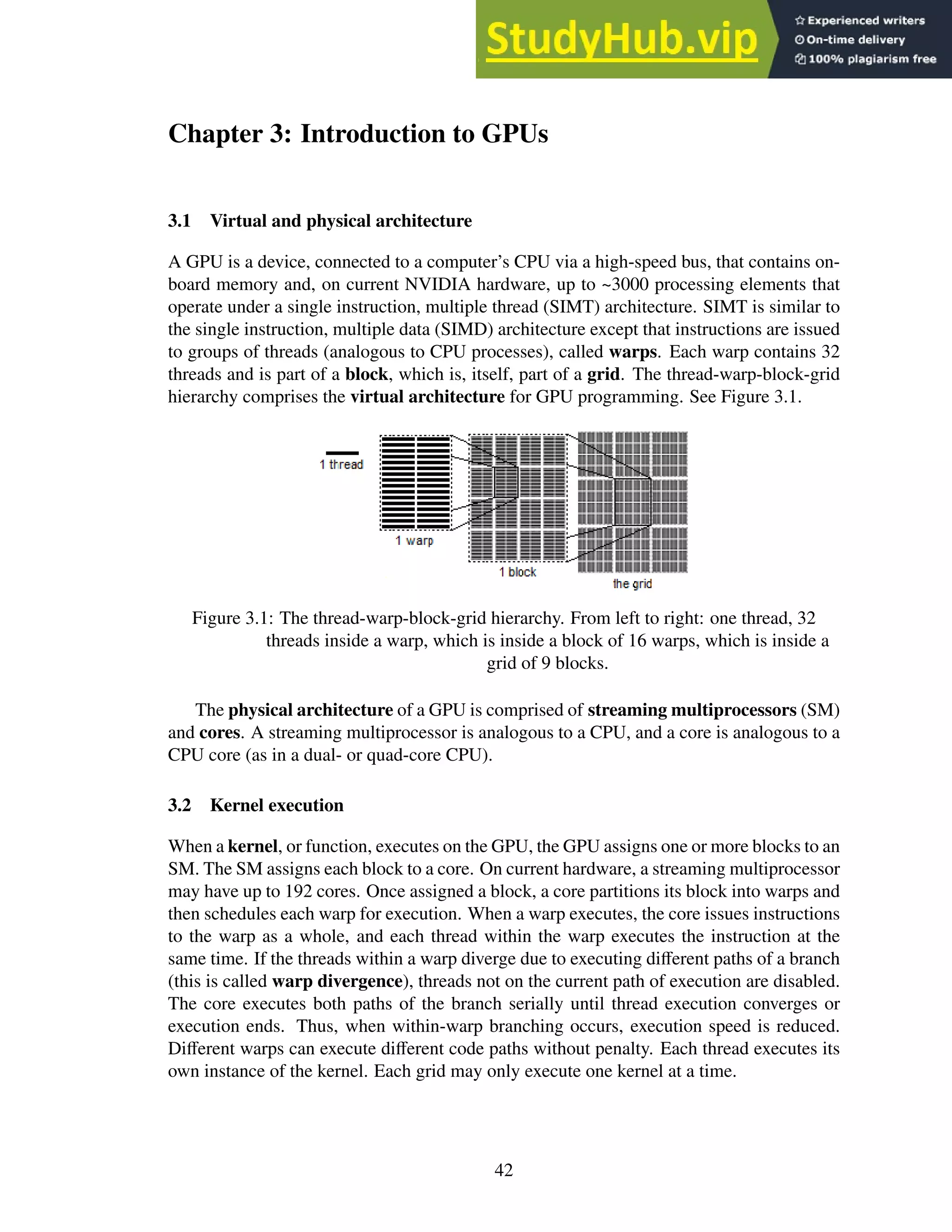
3.1 The thread-warp-block-grid hierarchy. From left to right: one thread, 32 threads
inside a warp, which is inside a block of 16 warps, which is inside a grid of 9
blocks. . . . . . . . . . . . . . . . . . . . . . . . . . . . . . . . . . . . . . . . 42
3.2 Example CUDA program modified from the NVIDIA CUDA C Programming
Guide [34]. . . . . . . . . . . . . . . . . . . . . . . . . . . . . . . . . . . . . 44
4.1 A graphical representation of Version 1 of the SegRec algorithm. . . . . . . . . 49
4.2 A glyph broken into a 3×3 grid . . . . . . . . . . . . . . . . . . . . . . . . . . 50
4.3 The edge-walk algorithm in the second version of SegRec. . . . . . . . . . . . 51
4.4 A kerned glyph with the grid-and-count grid and bounding polygon. . . . . . . 52
4.5 Examples of a glyph in which (a) reaching the starting point in an edge walk
does not indicate being finished and (b) where the edge walk completes normally. 53
4.6 Figure 4.5 highlighting the paths the edge-walk algorithm finds. . . . . . . . . 54
4.7 The pixel configurations fo which extra processing is necessary to detect the
appropriate next step for the edge-walk algorithm. . . . . . . . . . . . . . . . . 54
4.8 Two groups of black pixels. The red pixels show the divide between the groups. 56
4.9 Three glyphs with their bounding polygons highlighted. The coordinates high-
lighted are what would be stored in the bound arrays. . . . . . . . . . . . . . . 57
4.10 Process a byte of image data. . . . . . . . . . . . . . . . . . . . . . . . . . . . 58
4.11 An example of a thread processing a stripe. The blue pixels have been pro-
cessed and the red pixel is under consideration. . . . . . . . . . . . . . . . . . 59
4.12 An example glyph divided into strips. . . . . . . . . . . . . . . . . . . . . . . 59
4.13 A glyph encircled by a polygonal bounding box. . . . . . . . . . . . . . . . . . 61
4.14 Sample paths showing the different comparison types for the compression stage. 63
4.15 The results of merging the example paths. . . . . . . . . . . . . . . . . . . . . 63
4.16 The bounding polygon for the example. . . . . . . . . . . . . . . . . . . . . . 65
4.17 Three glyphs. . . . . . . . . . . . . . . . . . . . . . . . . . . . . . . . . . . . 66
4.18 The paths stored in the bounds arrays. The red paths are stored in S 1 and the
blue paths in S 0. . . . . . . . . . . . . . . . . . . . . . . . . . . . . . . . . . . 67
4.19 Sample XML output. . . . . . . . . . . . . . . . . . . . . . . . . . . . . . . . 71
5.1 (a) Original characters. (b) Characters with added noise. . . . . . . . . . . . . 73
5.2 A graph of the total time each engine spent per number of pages in seconds.
These metrics include time for reading the images from the hard drive and
copying data to and from the GPU. . . . . . . . . . . . . . . . . . . . . . . . . 75
5.3 A graph of the micro-f score for each engine versus each set of images. . . . . . 75
5.4 A graph of the macro-f score for each engine versus each set of images. . . . . 76
5.5 A graph of the time SegRec v3 spent per page in milliseconds versus number of
pages. These metrics include time for reading the images from the hard drive
and copying data to and from the GPU. . . . . . . . . . . . . . . . . . . . . . . 76
viii](https://image.slidesharecdn.com/anopticalcharacterrecognitionengineforgraphicalprocessingunits-230805215723-24ac1bd2/75/An-Optical-Character-Recognition-Engine-For-Graphical-Processing-Units-11-2048.jpg)

![Chapter 1: Introduction
1.1 Motivation
This dissertation describes research and development for an optical character recognition
(OCR) engine that runs on a graphical processing unit (GPU). The purpose of this en-
deavor is to significantly increase the speed of the image-processing and glyph-recognition
steps while maintaining accuracy and precision measures that favorably compare to exist-
ing commercial engines.
OCR was first introduced in the early 1900s as a technology designed to enable sight-
impaired people to read. The “Type-reading Optophone”, introduced in 1914, converts light
reflected off of type-written text into sounds — each glyph emitting a unique tone. With
training, a person could learn to discern the tones and “read” the text [11]. A later invention,
patented in 1931 and dubbed the “Statistical Machine”, was designed to help speed the
search for text in microfilm archives [16]. A light source positioned below the microfilm
and “search plates”, solid, opaque plates with the search text carved out, positioned above
the microfilm provides a variable light-source to a light detector positioned above the search
plate. As the microfilm moves, the light level above the search plate varies such that when
the text matches exactly with the search plate, very little light passes through the film to the
detector. The detector then records the occurrence as a possible text match [16].
This dissertation describes an OCR engine that processes glyphs that have already been
captured in image form, but much of the same process occurs as in the devices described
previously. Modern optical character recognition can be segmented into four main phases:
pre-processing, isolation, identification and post-processing. The pre-processing phase
prepares the image for the next phase and includes such tasks as noise reduction and ro-
tation correction. The isolation phase deals with dividing an image into sub-images, de-
lineating where lines, words and, ultimately, characters begin and end. The identification
phase accepts the output from the isolation phase and attempts to recognize the sub-images
passed to it as characters. The post-processing phase attempts to reassemble the charac-
ters into words and sentences. The main focus of this dissertation is on the isolation and
identification phases.
1.2 Contribution
In this dissertation, I present a series of algorithms for quickly isolating and identifying
characters from a large number of images containing typewritten text. As a whole, this
work comprises a framework for a GPU-enabled OCR engine.
During my research, I invented a number of algorithms:
• PathFind is a path-finding algorithm that operates on bi-tonal images and requires
no recursion or complex data structures. PathFind is discussed on page 18.
1](https://image.slidesharecdn.com/anopticalcharacterrecognitionengineforgraphicalprocessingunits-230805215723-24ac1bd2/75/An-Optical-Character-Recognition-Engine-For-Graphical-Processing-Units-14-2048.jpg)

![Rotation detection, estimation and correction
The whole image can be rotated, lines can be skewed or individual letters can be skewed.
The OCR algorithm must recognize the transformation and correct it prior to identification.
Alternatively, the identification phase must be aware of the transformation and adjust its
training data or other internal recognition mechanisms accordingly.
2.4 Pre-processing phase: Techniques and solutions
Thresholding
All thresholding1
techniques fall under the class of “data-reduction” algorithms. That is,
the techniques seek to compress or reduce the information contained within a given image
in order to reduce computational complexity. The purpose then, is to remove or reduce
the unwanted information or “noise” and leave the “important” information intact, such as
removing the background of a bank check so the OCR application can read the signature
panel.
For OCR applications, data reduction is usually confined to reducing a grayscale or
color image to a black and white (binary or bi-tonal) image. This reduction is accomplished
by calculating a level of intensity against which individual pixel values are compared. The
values that fall below the threshold are included in the binary image as black pixels; the
others are white [48]. The threshold value can be calculated on a global or local level, and
the techniques implementing each method are referred to as global or adaptive2
threshold-
ing, respectively. Global methods calculate the threshold using the entire image, whereas
local or adaptive thresholds readjust the threshold based on the area of the image around
which processing is taking place [4]. Adaptive techniques typically calculate a “running
value” for the threshold and make the black or white decision based on comparisons against
this value [56].
These thresholding techniques are also appropriate for removing bleed-through text,
because such text generally appears on the page at a much lighter contrast than normal text.
However, for severely degraded text or in cases where a document exhibits both varying
degrees of contrast and bleed-through text, thresholding is usually avoided [5].
1. Histogram-based thresholding techniques build a histogram of grayscale values and then
analyze the histogram topology. The analysis finds groups of peaks that are then com-
bined by averaging the grayscale values within the group, thereby reducing the total
number of grayscale values. Figure 2.1 shows an example of this method. Figure 2.1a
contains 6 grayscale values. The histogram groups the peaks. Averaging the groupings
results in the image Figure 2.1c, which gives a reduction in grayscale values of 50%
[46].
2. The clustering technique (or Otsu’s method) attempts to find the threshold that sepa-
rates the grayscale values into classes that maximize the between-class variance [37]. In
simpler terms, the technique attempts to find the histogram grouping that maximizes the
1
Also referred to as binarization.
2
Also referred to as local thresholding.
6](https://image.slidesharecdn.com/anopticalcharacterrecognitionengineforgraphicalprocessingunits-230805215723-24ac1bd2/75/An-Optical-Character-Recognition-Engine-For-Graphical-Processing-Units-19-2048.jpg)
![(a) (b)
(c) (d)
Figure 2.1: The original image with 6 grayscale values (a) and its histogram (b). The
reduced image with 3 grayscale values (c) and its histogram (d).
difference in intensity between two groups of grayscale values. In the final grouping,
the lighter values are drawn as white pixels and the darker values as black pixels. The
threshold is the value that splits the class groupings.
Singh et al. parallelized Otsu’s method for an average speedup of 1.6× over serial meth-
ods [51].
3. Entropy methods select a threshold based upon entropic calculations performed on the
histogram [3, 8, 21]. In the simplest form, the chosen threshold splits the pixel count
equally, as entropy is maximized when a pixel is equally as likely to be black as it is to
be white. See Figures 2.3 and 2.4.
4. An object-attribute method examines a particular attribute of an object (in this case,
a glyph) and utilizes some specific feature of that object to perform a function. An
example of such an algorithm utilizes edge detection to perform thresholding. First, the
algorithm applies a heuristic to choose the initial threshold values based upon the peak
values within the grayscale histogram of the image. Next, an edge detection routine runs
on both the original image and the thresholded image. If the edges match, the thresholds
are kept and the process is complete. If not, the image is broken down into smaller
chunks and the whole process repeats. Thus, this technique utilizes global thresholding
at the beginning and selectively applies adaptive thresholding as the need arises [19].
7](https://image.slidesharecdn.com/anopticalcharacterrecognitionengineforgraphicalprocessingunits-230805215723-24ac1bd2/75/An-Optical-Character-Recognition-Engine-For-Graphical-Processing-Units-20-2048.jpg)
![Figure 2.4: Original image after the threshold from Figure 2.3 is applied.
5. A dynamic algorithm, called the integrated function algorithm, is able to separate
text from backgrounds with as little as 20% difference in contrast. The algorithm first
identifies edges of sharp contrast (similar to the previous method) and then assumes
that character strokes range in width from 0.2mm to 1mm in order to determine if an
identified region is a character or an area of high-contrast background. The algorithm
marks regions identified as characters black and all other regions as white [55].
6. The basic adaptive thresholding technique is called the Niblack binarization algo-
rithm. The algorithm works by calculating the threshold value within a sliding window
using the mean and the standard deviation and includes or excludes the pixels in the area
according to the calculated value. The window shape is up to the implementation and
can vary based upon the requirements of the images being processed [31]. Sauvola’s
algorithm modifies Niblack to store and use the dynamic range of standard deviation,
which adapts the threshold to ignore noisy backgrounds [45].
Singh et al. parallelized Niblack’s binarization algorithm for a speedup of 20× to 22×
over serial methods [50]. Singh et al. and Chen et al. also parallelized Souvala’s algo-
rithm for a speedup of 20× to 22× and 38×, respectively, over serial methods [9, 52].
7. A variation on Niblack’s algorithm is pixel density thresholding. This method deter-
mines the average pixel density within a sliding window and includes or excludes the
pixels in that area accordingly. The window shape is up to the implementation and
can vary based upon the requirements of the images being processed. This technique
is useful for removing streaks and marks due to poor image quality and can also oper-
9](https://image.slidesharecdn.com/anopticalcharacterrecognitionengineforgraphicalprocessingunits-230805215723-24ac1bd2/75/An-Optical-Character-Recognition-Engine-For-Graphical-Processing-Units-22-2048.jpg)
![ate in conjunction with another thresholding algorithm. The pixel density thresholding
technique is not mentioned in any paper I have found.
(a) (b)
(c) (d)
(e)
Figure 2.5: (a) and (c) show the two chain code scoring methods; (b) and (d) show a
sample chain using their respective scoring methods; (e) shows an ‘a’ and its
corresponding chain code. The arrow denotes the starting position for each
chain code.
8. Another algorithm for a noise-reduction thresholding technique is called chain code
thresholding. A chain code is a data structure that consists of a start point and a string
of digits representing a list of directions. The digit string contains numerals in the range
0-7 (or 0-3) that represent all possible directions on a 2D image. A chain code is formed
by choosing a starting point, moving one pixel in an allowed direction and appending
that direction to the digit list. Thus, the chain code is a representation of a path in 2D
space. Chain code thresholding constructs chain codes representing the border of each
pixel group and analyzes the resultant digit string. During the isolation phase, if a chain
code has a length below a certain threshold, it can be discarded. This method is not
mentioned in the literature, though chain codes are described in detail by Freeman [14].
10](https://image.slidesharecdn.com/anopticalcharacterrecognitionengineforgraphicalprocessingunits-230805215723-24ac1bd2/75/An-Optical-Character-Recognition-Engine-For-Graphical-Processing-Units-23-2048.jpg)
![DIBCO, the Document Image Binarization Contest, was started in 2009 in order to
evaluate and test the best thresholding techniques [1]. The contest ran from 2009 through
2014. The winning entries for each year are all hybrid algorithms that break down the
thresholding process and use the best-of-breed algorithm for each part. For example, the
winning submission in 2009 was by Lu et al., a team from the Institute for Infocomm
Research in Singapore. Lu’s submission incorporates Otsu’s method, Niblack’s algorithm,
stroke edge detection and a post-process clean-up step [15]. Unfortunately, the published
results from 2010 to 2014 are too brief to glean any meaningful detail about the algorithms.
However, I include references for each of the yearly result papers for completeness: 2009
[15], 2010 [40], 2011 [41], 2012 [42], 2013 [43], and 2014 [32].
Otsu’s method provides an excellent general-purpose algorithm for thresholding that
many authors still reference as a baseline for comparing their methods. However, advance-
ments made in adaptive thresholding, such as the object-attribute edge detection and the
integrated function algorithms described above, and increased document complexity limit
the appeal of global thresholding as a whole. This shift to adaptive algorithms is because
the cost of each type of algorithm is similar, but the adaptive methods handle contrast gradi-
ents and variations within documents better. Ultimately, choosing a thresholding algorithm
is context- and domain-specific. For example, Otsu’s method is a simple, parameterless
algorithm that will give good results on documents with high contrast between text and
background, whereas the adaptive methods, such as the integrated function algorithm, are
more complex, require tuning and are required only for more complex documents.
Rotation detection, estimation and correction
There are four basic types of rotation-detection algorithms: projection profile, nearest
neighbor clustering, component labeling, and the Hough transform [12].
Figure 2.6: Horizontal and vertical projection profiles. Figure recreated from Abdelwahab
et al. [56].
1. The projection profile technique projects the document at different angles, then, for
each angle, constructs a graph based on the sum of black pixels in each line. Peaks
are due to scanlines with high pixel density and troughs are due to white space and
scanlines with low pixel density. The document angle that gives the maximum difference
between the peaks and troughs is the rotation angle [12]. This technique can be applied
horizontally or vertically. The horizontal application of the projection profile technique
works better for the languages written in rows (i.e. right to left or left to right), such as
English, whereas the vertical application works better for languages written in columns,
such as Chinese. See Figure 2.6.
11](https://image.slidesharecdn.com/anopticalcharacterrecognitionengineforgraphicalprocessingunits-230805215723-24ac1bd2/75/An-Optical-Character-Recognition-Engine-For-Graphical-Processing-Units-24-2048.jpg)
![2. The nearest-neighbor clustering method constructs “pixel groups” from directly con-
nected pixels. Every pixel group contains at least one glyph (this technique assumes
there are no groups with only noise). The method calculates the vertical center of each
pixel group and uses it to calculate the angle between the closest pixel groups and a hor-
izontal reference line. Next, the algorithms constructs a histogram from these results,
and the angle found to be most common, indicated by the highest peak in the histogram,
is the rotation angle [12]. See Figure 2.7.
Figure 2.7: Nearest-neighbor clustering uses the angle between pixel groups to compute
rotation. In this example, the glyphs themselves form the pixel groups.
3. Component labeling, a technique adapted from graph theory, attempts to calculate the
average height of the characters in a line in order to identify the mean line and baseline.
Once identified, these lines can be used to calculate the rotation. The mean line is
roughly defined as the equivalent to the top of a lowercase character, excluding those
characters with ascenders or descenders (e.g. d, t, g, y, etc.). The baseline is the line
upon which the characters are printed. The algorithm groups and labels sets of pixels as
belonging to either the mean line, baseline or neither by maintaining a running average
for the height of a character and excluding outliers, such as tall characters, marks, and
letters with ascenders or descenders. Once the process is complete and the average
height is known, the mean line and baseline estimate the rotation angle [12].
Figure 2.8: Depiction of the mean line and base line. Figure recreated from Das et al. [12].
4. The Hough transform also attempts to discover the mean lines and baselines in an im-
age of text as a way to calculate rotation. The algorithm maintains a two-dimensional
array indexed by line slope and origin that functions as an accumulator. A naïve imple-
mentation of the transform projects lines at varying angles through each black pixel and
counts the number of intersections with other black pixels. If the number of intersections
is above a threshold, the algorithm increments the corresponding slots for the line angle
and origin within the accumulator array. This algorithm operates under the assumption
that the mean lines and baselines for a given page of text have the highest pixel density.
The angle represented by the bucket with the highest value is taken as the angle of either
12](https://image.slidesharecdn.com/anopticalcharacterrecognitionengineforgraphicalprocessingunits-230805215723-24ac1bd2/75/An-Optical-Character-Recognition-Engine-For-Graphical-Processing-Units-25-2048.jpg)
![the mean line or the base line (or both) and is the rotation angle [29]. This algorithm can
be applied on a global or local scale. The main drawback for implementing the Hough
transform is its computational complexity [12]. See Figure 2.9.
Figure 2.9: The Hough transform projects lines through pixels and counts the intersections
to find the mean line and the baseline.
5. The Das and Chanda morphology method calculates rotation by performing the mor-
phological close operation (described below) with a 12×1-pixel horizontal line struc-
turing element to reduce each line of text into a black band. The algorithm smooths
each band with a morphological open operation (described below) and marks the bot-
toms with a line. The algorithm measures these lines and averages their rotations. The
average of the angles is the rotation angle.
A morphological close operation works by sliding a structuring element across a binary
image. Everywhere the structuring element overlaps only white pixels remains white;
the white pixels where the element does not fit are made black. See Figure 2.10.
(a) (b)
Figure 2.10: An example 2×2-pixel morphological close operation. (a) the original shape,
(b) the shape after the structuring element is applied.
After the algorithm applies the 12×1-pixel horizontal line structuring element via the
morphological close, each black band contains rough edges corresponding to the pres-
ence of ascenders and descenders. The algorithm smooths these bumps by applying the
morphological open operation with a 5×5-pixel structuring element. The open opera-
tion works like the close operation, except instead of sliding around on the white pixels,
the algorithm places the open structuring element on the black pixels in an image. Ev-
erywhere the opening structuring element fits, the pixels remain black; the black pixels
where the element does not fit are made white. See Figure 2.11.
Once the black bands are smoothed, the algorithm scans the document top to bottom
and marks black to white transitions. Essentially, this step captures the baseline of each
text line. If the line length exceeds some threshold, the angles of the lines are measured
and averaged and the resultant angle is the rotation angle [12]. See Figure 2.12 on page
14.
13](https://image.slidesharecdn.com/anopticalcharacterrecognitionengineforgraphicalprocessingunits-230805215723-24ac1bd2/75/An-Optical-Character-Recognition-Engine-For-Graphical-Processing-Units-26-2048.jpg)
![(a) (b)
Figure 2.11: An example 2×2-pixel morphological open operation. (a) the original shape,
(b) the shape after the structuring element is applied.
(a) (b)
(c) (d)
Figure 2.12: The Das and Chanda morphology method. (a) the original text, (b) the text
after the close operation using a 12 pixel horizontal structuring element. (c)
the text after the open operation with a 5 pixel x 5 pixel structuring element.
(d) the transitions from black to white pixels, representing the baseline of the
text.
6. The bounding-box reduction method subdivides the image into sections by global and
adaptive thresholding, then attempts to reduce the bounding boxes around each subsec-
tion through a brute-force rotation mechanism. The algorithm rotates each subsection of
the document by a step angle, then re-calculates the bounding box for that subsection.
The algorithm accepts the angle that minimizes the overall area of the bounding box as
the rotation angle for that subsection. This method allows for multiple rotation angles to
be present on a document. This method also works on documents that include graphics,
as each graphic is treated as just another subsection [4]. See Figure 2.13.
All these algorithms are adequate at finding the rotation angle on a rotated document.
Typical results from each of the corresponding references report deviations from the actual
rotation value of less than several tenths of a degree. However, the clear winner is the
bounding-box reduction method. This algorithm can be used with mixed graphics and text
documents and can handle multiple rotation angles on the same page, since it processes
each section separately. For text-only documents, the Das and Chanda morphology method
is viable, though the implementation depends heavily on the efficiency of the open and
close morphology operations.
In general, the rotation angle in scanned text tends to be less than a few degrees and,
in such cases, a shear transformation (or shear mapping) is an efficient corrective measure;
rotation is much more expensive.
14](https://image.slidesharecdn.com/anopticalcharacterrecognitionengineforgraphicalprocessingunits-230805215723-24ac1bd2/75/An-Optical-Character-Recognition-Engine-For-Graphical-Processing-Units-27-2048.jpg)
![Kerning
Some fonts and handwriting styles contain characters that project into the vertical space
of surrounding characters, which makes isolating individual characters more complex as
compared to fonts with clearly separated characters. For example, the characters “WJ’ are
not separated by vertical white space.
Character ligatures
Ligatures are strokes that connect one letter to another. Small fonts, cursive English hand-
writing and Arabic all exhibit characters that are connected via a continuous stroke. Con-
nected characters are hard to separate.
Marks
In many languages, letters have various accents and accompanying strokes (marks) that
are unconnected to the rest of the letter, such as the dot in the English lower case ‘i’.
Because the meaning of a glyph can change based on these marks, the OCR application
must correctly group them with the base. Marks can appear above or below a base.
Complex page layout
If a page is multi-columnar or contains sidebars of text or textual graphics such as solid
lines separating sections, the OCR application needs to be able to group the appropriate
lines of text together and discard the graphics as noise.
2.6 Isolation phase: Techniques and solutions
Kerning
1. Chain codes representing boundaries are an effective way to capture entire characters
even if they are kerned. The chain code moves around the border, operating on either the
black pixels of the character itself or the white pixels directly adjacent to the character,
until the entire character has been enveloped. This algorithm fails if characters are not
separated by white space.
2. An alternative method is to find the best-fit bounding box. A best-fit bounding box is a
rectangle that surrounds the character and is bounded by the most likely horizontal loca-
tion where one character ends and another begins. An algorithm finds these locations by
calculating the horizontal and vertical pixel density of the area and choosing the valley
locations [28]. These bounding boxes may intersect and include portions of other char-
acters, so this method requires additional processing to remove any extra pixels caused
by this inclusion. Noise reduction algorithms, such as chain-code thresholding, can re-
move the extra pixels. An enhancement to the algorithm is to calculate the average size
of each letter and impose minimum and maximum widths (or heights) for the bounding
box. See Figure 2.16.
16](https://image.slidesharecdn.com/anopticalcharacterrecognitionengineforgraphicalprocessingunits-230805215723-24ac1bd2/75/An-Optical-Character-Recognition-Engine-For-Graphical-Processing-Units-29-2048.jpg)
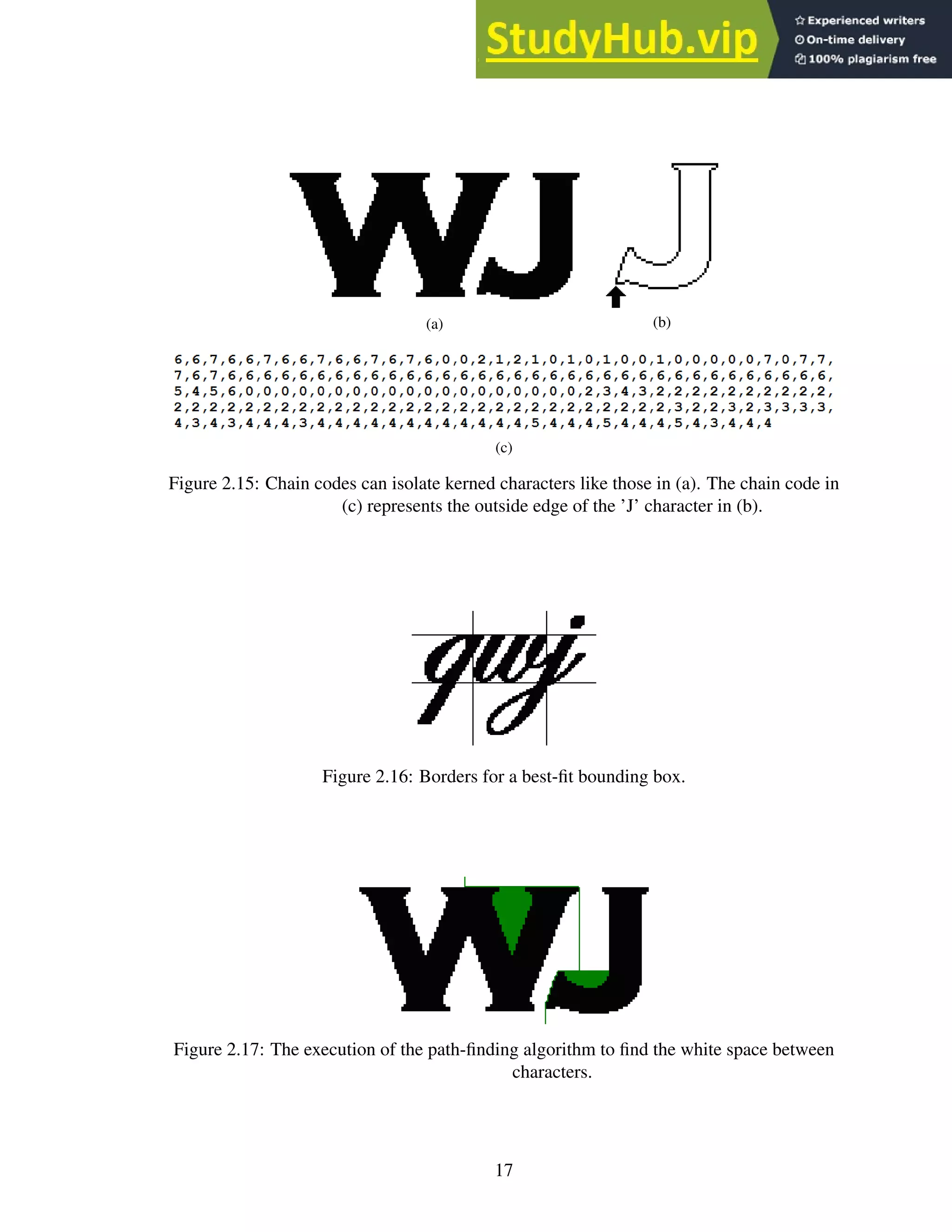
![3. Another method is to find a path between kerned characters. This method creates a
bounding polygon that isolates the characters from each other. The downside to this
algorithm is its computational complexity.
I developed a pathing algorithm, PathFind, that operates on a bi-tonal image as shown in
Figure 2.18 on page 19. This path-finding algorithm requires no recursion or complex
data structures, results in an array of fixed size, requires no target ‘end point’ (it only
tries to find a path to some x at image_height − 1), and requires very little memory.
These features make it especially good for GPU processing.
Of the methods described, the PathFind algorithm seems to be the most likely candi-
date for a general-purpose solution. The best-fit bounding box suffers from the problem of
determining where the “best-fit” actually occurs. For example, in the case of Figure 2.16
on page 17, a reasonable alternative for a best-fit box may only capture half the “w”. The
algorithm using chain codes must check and process every pixel on the border of a glyph
and must convert a finished chain code into a bounding polygon, which generally requires
more processing than the PathFind algorithm (the cost of the chain code algorithm is pro-
portional to the border length of a glyph; the cost of PathFind is proportional to the height
of a glyph).
Marks
1. The only technique in the literature for dealing with marks is to use the overall height-to-
width ratio to determine if a mark belongs with a particular character [29]. If pairing the
mark with a specific character increases the height-to-width ratio of the character beyond
a threshold, the mark is excluded; otherwise it is included with the character. Since most
marks are placed above or below their bases, this method is particularly effective. The
OCR engine could also try to recognize the character both with and without the mark,
accepting whichever version is recognized. If both versions are recognized, confidence
values can be relied upon to determine a winner. The OCR engine could also recognize
marks and bases separately and combine them in post-processing.
2. Using the bounding boxes of isolated glyphs, one can easily compute the distance be-
tween smaller boxes (most likely marks) to the nearest larger box (most likely a base) to
determine to which base the mark belongs. This technique allows the creation of entire
characters from the constituent strokes in the image. This method is not mentioned in
the literature.
This problem needs more research, because there is no good generic algorithm for
associating marks with their base. The lack of any generic algorithm is probably because
the types of marks seen in an alphabet vary widely with the alphabet under consideration,
so any generic algorithm would need to account for this variability. An algorithm could
be derived from the bounding-box idea described above, though heuristic workarounds
would be necessary for some alphabets. If the algorithm is processing a language where
there are no marks under the baseline, English for example, it would never need to consider
character bases above the mark. However, for a language such as Hebrew, bases both above
and below the mark are candidates.
18](https://image.slidesharecdn.com/anopticalcharacterrecognitionengineforgraphicalprocessingunits-230805215723-24ac1bd2/75/An-Optical-Character-Recognition-Engine-For-Graphical-Processing-Units-31-2048.jpg)
![1 int x_arr[IMAGE_HEIGHT];
2 // y increases downward, the origin is at the top-left
3 int cur_y = 1;
4 //starting x-value is the middle of the glyph
5 x_arr[0] = IMAGE_WIDTH / 2;
6 while (cur_y < IMAGE_HEIGHT) {
7 if (GetPixel(x_arr[cur_y], cur_y + 1) == White)
8 { // down
9 x_arr[cur_y + 1] = x_arr[cur_y];
10 cur_y = cur_y + 1;
11 MarkPixel(x_arr[cur_y], cur_y);
12 }
13 else if (GetPixel(x_arr[cur_y] + 1, cur_y + 1) == White)
14 { // down right
15 x_arr[cur_y + 1] = x_arr[cur_y] + 1;
16 cur_y = cur_y + 1;
17 MarkPixel(x_arr[cur_y], cur_y);
18 }
19 else if (GetPixel(x_arr[cur_y] - 1, cur_y + 1) == White)
20 { // down left
21 x_arr[cur_y + 1] = x_arr[cur_y] - 1;
22 cur_y = cur_y + 1;
23 MarkPixel(x_arr[cur_y], cur_y);
24 }
25 else if (GetPixel(x_arr[cur_y] + 1, cur_y) == White)
26 { // right
27 x_arr[cur_y] = x_arr[cur_y] + 1;
28 MarkPixel(x_arr[cur_y], cur_y);
29 }
30 else if (GetPixel(x_arr[cur_y] - 1, cur_y) == White)
31 { // left
32 x_arr[cur_y] = x_arr[cur_y] - 1;
33 MarkPixel(x_arr[cur_y], cur_y);
34 }
35 else if (cur_y == 0)
36 { // no path, stop
37 return;
38 }
39 // we have checked the right path
40 // so we reset so to check the left path
41 else if (GetPixel(x_arr[cur_y - 1] - 1, cur_y - 1) == White)
42 {
43 x_arr[cur_y] = x_arr[cur_y - 1];
44 }
45 else
46 { // backtrack
47 cur_y = cur_y - 1;
48 }
49 }
Figure 2.18: PathFind pseudo code.
19](https://image.slidesharecdn.com/anopticalcharacterrecognitionengineforgraphicalprocessingunits-230805215723-24ac1bd2/75/An-Optical-Character-Recognition-Engine-For-Graphical-Processing-Units-32-2048.jpg)
![Character ligatures
1. The best-fit bounding box is the only method in the surveyed literature for determining
where to separate characters connected via ligatures [28]. See Figure 2.16 on page 17
for an example.
Figure 2.19: Possible vertical boundary borders of a best-fit bounding box.
2. An alternative method is to calculate the vertical pixel density of the text line and then
create a set of best-fit bounding boxes. Each member of the set corresponds to a bound-
ing box with borders that fall in the valleys for the vertical density graph, as in Figure
2.19. Each set of borders is processed as a best-fit bounding box (with noise reduction,
partial character removal, etc.) and the boxes that are found to contain valid characters
are kept. This method is not mentioned in the literature.
Figure 2.20: Several potential chop points that the Tesseract OCR engine might use to
overcome ligatures. Figure recreated from Smith [53].
3. A method suggested by the Tesseract OCR engine is to determine “chop points” or thin
points on a glyph. The glyphs are then separated at the chop points and recognition is
attempted on the pieces [53].
Complex page layout
1. The x-y cut segmentation algorithm uses recursion to construct a tree-based represen-
tation of the document, with the root as the whole document and each leaf comprising
a single section of similar content (text, graphics, etc.) from the image. First, the algo-
rithm computes the horizontal and vertical projection profile (see Figure 2.6 on page 11)
of the document and splits it into two or more segments based on the valleys in the den-
sity graphs. In Figure 2.21, the vertical density graph shows two potential split points
corresponding to the white space between the columns, and the horizontal density graph
20](https://image.slidesharecdn.com/anopticalcharacterrecognitionengineforgraphicalprocessingunits-230805215723-24ac1bd2/75/An-Optical-Character-Recognition-Engine-For-Graphical-Processing-Units-33-2048.jpg)
![Figure 2.21: A complex page layout with horizontal and vertical projection graphs.
Valleys in the graphs show potential split points.
shows many potential split points, one between each line. Once split, these segments are
connected as children to the root node. Then, for each newly created child, the process
recurses. When no more splits can be made, the algorithm is finished [13, 47].
Singh et al. [49] implemented a version of the x-y cut algorithm for segmenting De-
vanagari text lines and words. The paper did not provide a clear explanation of their
implementation, but, according to their results, the authors saw a 20× to 30× speedup
over serial methods.
2. The smearing algorithm operates horizontally or vertically on binary images by “smear-
ing” the black pixels across white space if the number of consecutive white pixels falls
below some threshold. This algorithm has the effect of connecting neighboring black
areas that are separated by less than a threshold value. Connected-component analysis
connects the smeared pixel groups to form segments, and the set of segments comprises
the page layout. Typically, horizontal smearing works best for alphabets written hori-
zontally, such as English [47]. See Figure 2.22.
3. White-space analysis finds a set of maximal rectangles whose union is the complete
background. The rectangles are sorted according to their height-to-width ratios, with
21](https://image.slidesharecdn.com/anopticalcharacterrecognitionengineforgraphicalprocessingunits-230805215723-24ac1bd2/75/An-Optical-Character-Recognition-Engine-For-Graphical-Processing-Units-34-2048.jpg)
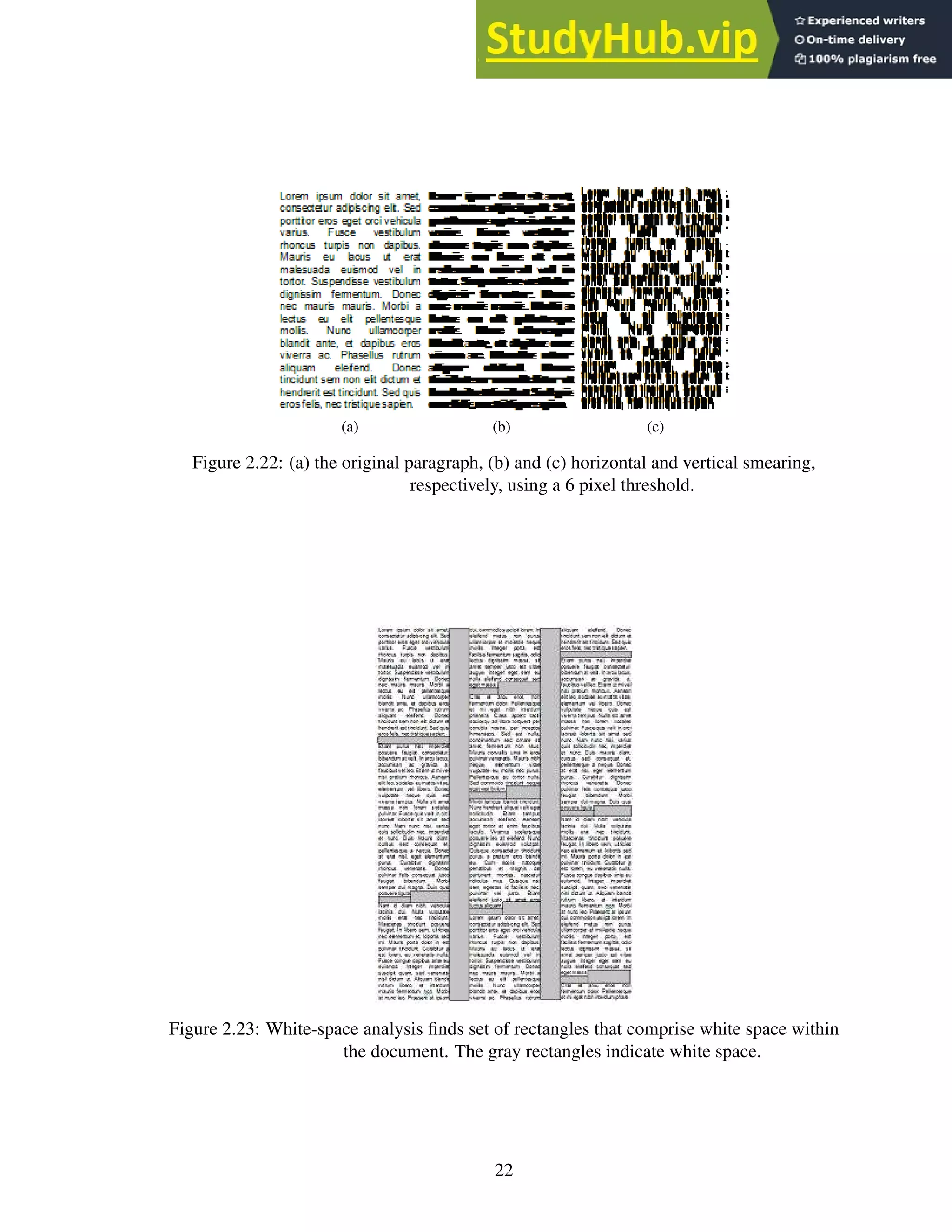
![an additional weight assigned to tall and wide blocks, since these blocks typically rep-
resent breaks between text blocks. Figure 2.23 depicts “tall” blocks between columns
and “wide” blocks between paragraphs. The blocks left uncovered are the text-block
segments [47].
4. The Docstrum algorithm is based on nearest-neighborhood clustering of connected
components. The algorithm partitions the connected components into two groups, one
with characters of the dominant font size, and one with the remaining characters. For
each component, the algorithm identifies k nearest neighbors and calculates the distance
and angle to each neighbor. The neighbors with the shortest distance and smallest angles
are considered to be on the same line. The whole text line is determined by combining
the series of these within-line pairings. The final text block segmentation is formed by
merging text lines based on location, similar rotation angles and line lengths [47].
5. The area Voronoi diagram method is based on the concept of Voronoi diagrams. In
the simplest case, a Voronoi diagram on an x-y plane consists of a set of regions, each
containing a center point and a set of points such that the distance from each point to the
center point is less than the distance from that point to any other center point. The sim-
plest measure is Euclidean distance, but other measures can be used. See Figure 2.24.
The algorithm creates Voronoi regions around each character glyph. The algorithm re-
moves boundaries between regions that are below a minimum distance from each other.
It also removes boundaries between regions whose area is similar in order to cover cases
where images contain graphics and figures. The underlying idea is that, for any individ-
ual character, the area of the Voronoi region is roughly the same, whereas the area for a
graphic or figure is much larger [23].
There is no clear choice for the best page-segmentation algorithm; each has merits un-
der certain document conditions. To summarize the results of the performance evaluation
by Shafait et al. [47]: the x-y cut algorithm is best for clean documents with little to no ro-
tation; the Docstrum and Voronoi algorithms are appropriate for homogeneous documents
that contain similar font sizes and styles; white-space analysis works well on documents
containing many font sizes and styles; and the Voronoi method excels at segmenting page
layouts with text oriented in different fashions [47].
Multiple colors
I was unable to locate any papers describing methods to handle multiple-colored docu-
ments, though one can hypothesize ways to remove solid-color backgrounds and deal with
different-colored foregrounds. One naïve method is to separate a full color image into 3
sub-images, each sub-image containing only the R, G or B color components. Convert
these sub-images to grayscale, then process each of them as a normal grayscale image and
combine the results.
Figure 2.25 contains an example of splitting the R, G and B components from a full-
color image. The colors in the original image, Figure 2.25a, comprise the full list of colors
created by using all combinations of the values 0, 64, 128, 192 and 255 for each component.
23](https://image.slidesharecdn.com/anopticalcharacterrecognitionengineforgraphicalprocessingunits-230805215723-24ac1bd2/75/An-Optical-Character-Recognition-Engine-For-Graphical-Processing-Units-36-2048.jpg)
![The text color is the negative color of the background. The components of the negative
color are calculated as 255 − original_component.
For each component image, the algorithm performs adaptive thresholding to convert
the grayscale image to monochrome. To determine which pixels are the “text pixels”, it
might analyze the histogram and look for the most common value (black or white) —
presumably the background pixels comprise the majority of the image. For images such as
those in 2.25, a new analysis method might be useful — adaptive histogram analysis3
.
This method constructs a histogram for a section of an image in order to perform analysis
on that section. The analysis enables an application to adapt to multi-colored backgrounds
and successfully separate the text.
(a)
(b)
(c)
(d)
Figure 2.25: Multiple color image with negative color text and isolated color components,
(a) the original image, (b) the R component, (c) the G component, (d) the B
component.
3
This method is similar to adaptive histogram equalization, which is a technique used to improve
contrast in images and credited to Ketcham et al., Hummel and Pizer [20, 22, 38, 39]
25](https://image.slidesharecdn.com/anopticalcharacterrecognitionengineforgraphicalprocessingunits-230805215723-24ac1bd2/75/An-Optical-Character-Recognition-Engine-For-Graphical-Processing-Units-38-2048.jpg)
![2.7 Identification phase: Problems
The identification phase must account for deficiencies in the isolation phase. The problems
this phase must overcome are partial letters, multiple font types and handwriting styles,
character normalization, data extraction and the confusing character set.
Partial letters
Images scanned from books, handwritten documents or historical documents may contain
partially erased, occluded or faded letters. These letters must be recognized in their partial
state.
Multiple font types and handwriting styles
A font refers to the typeface of a particular set of characters. In machine-printed text and
handwritten text, all the various styles and ways to write each character must be recognized
as that specific character.
Character normalization
Often, recognition techniques require normalizing glyph image sizes to a standard image
size in order to match training data. The normalization technique can alter the recogni-
tion rate of the normalized glyph because of differences in the way the technique handles
thick fonts versus thin fonts or tall versus short fonts. Different sizes of fonts also tend to
have different relative stroke thicknesses, but a normalized character glyph maintains its
thickness ratio across scales [24].
Data extraction
The identification phase relies on extracting characteristic data from character glyphs that
can then classify the glyph as a specific character. There are two main options for char-
acter data extraction: feature extraction and image transformation. Feature extraction
techniques extract data directly from the glyph of a character. Image transformation
techniques transform the glyph into another representation, such as a waveform, and then
extract data from the transformed glyph.
The choice of features to extract or transformations to apply is crucial to OCR accuracy.
If character data are poorly extracted, too similar or insufficient, the OCR application may
misidentify the characters.
Confusing character set
The confusing character set contains those characters within a given alphabet and font that
are commonly misrecognized by OCR techniques. For English, the confusing character set
might contain: the uppercase ‘I’ and lowercase ‘l’ (lowercase ‘L’), the number ‘1’ and
lowercase ‘l’, the uppercase ‘O’ and the number ‘0’ and the lowercase ‘e’ and lowercase
‘c’.
26](https://image.slidesharecdn.com/anopticalcharacterrecognitionengineforgraphicalprocessingunits-230805215723-24ac1bd2/75/An-Optical-Character-Recognition-Engine-For-Graphical-Processing-Units-39-2048.jpg)
![2.8 Identification Phase: Techniques and solutions
Partial Characters and Multiple Font/Handwriting Types
Skeletonization or “thinning” is a technique that captures the overall shape of a character
by reducing each character stroke to one pixel wide. This process recreates the essence
of the “human” capability to reduce a shape to its constituent parts and capture the overall
shape. This method is able to handle multiple fonts and handwriting types since, theoreti-
cally, the algorithm removes the extra “noise” generated by different fonts and styles.
1. The generic process to skeletonize a character involves removing pixels from each side
of a stroke until only one pixel remains. This process “thins” the character while retain-
ing the overall shape [26]. The technique can be applied both horizontally and vertically.
See Figure 2.26.
Figure 2.26: The letter ‘A’ undergoing horizontal skeletonization. The gray pixels indicate
pixels selected for deletion.
2. Another method for skeletonization projects successively lower horizontal scanlines
across a character and then groups the lines as splitting, merging or continuous (see
Figure 2.27). A splitting line is a scanline that is split by white space, such as a line pro-
jected horizontally through the middle of an English ‘W’. A merging scanline is a line
directly adjoining (above or below) a group of split lines, indicating the character is no
longer split. All other lines are continuous. Adjoining lines of the same type are merged
into blocks. The vertical and horizontal center, called the centroid, of each block serves
as the representative of each block and acts an an endpoint for a connection path (see
Figure 2.28). Centroids that lie on the same vertical or horizontal as another centroid
are connected using a straight line; all others are connected using either a line with a
single 90 degree turn or a line with a single 120 degree turn. The lines are chosen to fit
within the blocks as much as possible while still connecting the centroids. The series of
connected centroids is the skeleton of the original character [26]. See Figure 2.29.
The idea behind skeletonization is to reduce the character glyph to its underlying form
such that multiple fonts reduce to the same structure. From the literature, the only algorithm
that does this reduction reliably is the method of Lakshmi et al. [26]. Unfortunately, the
computational complexity of this algorithm is quite large compared to other, less reliable
algorithms. More research needs to be done on this topic.
27](https://image.slidesharecdn.com/anopticalcharacterrecognitionengineforgraphicalprocessingunits-230805215723-24ac1bd2/75/An-Optical-Character-Recognition-Engine-For-Graphical-Processing-Units-40-2048.jpg)
![Figure 2.27: (a) the original character (b) horizontal runs (c) runs marked as splitting or
merging; unmarked runs are continuous (d) blocks (e) centroid computation
(f) connected centroids. Figure recreated from Lakshmi et al. [26].
Figure 2.28: Allowed connection paths. The sizes are not relative. Figure recreated from
Lakshmi et al. [26].
Figure 2.29: The calculated skeleton.
Figure 2.30: (a) a 72pt character scaled down to 36pt. (b) a 12pt character scaled up to
36pt. (c) an original 36pt character.
28](https://image.slidesharecdn.com/anopticalcharacterrecognitionengineforgraphicalprocessingunits-230805215723-24ac1bd2/75/An-Optical-Character-Recognition-Engine-For-Graphical-Processing-Units-41-2048.jpg)
![Character normalization
1. A simple method for character normalization is to scale the character based on the size
of the bounding box. Scaling a small font up does not perform as well as scaling a large
font down, due to missing pixel data (see Figure 2.30).
(a)
(b)
Figure 2.31: The black and white dots show the sampling positions. (a) the original
characters with various orientations within the image. (b) the resultant
scaled-down characters. Figure recreated from Barrera et al. [6].
a) Sampling is a down-scaling method that relies on sampling pixels in the horizontal
and vertical directions at a rate defined by the step. For example, a step of 2 means
that every second pixel is included in the sample, whereas a step of 3 means every
third pixel is included. Each sampled pixel is included to construct the final, scaled
down image. Depending on the position of a character at the start of the sampling
process, this method may result in varying shapes (see Figure 2.31).
b) Anchoring is a variation of the sampling method that computes an anchor point
for each character before sampling. The anchor point is the center of the bounding
box that contains the character and serves as the starting point for the sampling
process. By determining a standard starting point, the anchoring method results in
more consistent shapes [6].
Data extraction
There are many techniques for extracting features from character images. Successful OCR
applications combine a number of the following techniques. Rather than list them all, I
29](https://image.slidesharecdn.com/anopticalcharacterrecognitionengineforgraphicalprocessingunits-230805215723-24ac1bd2/75/An-Optical-Character-Recognition-Engine-For-Graphical-Processing-Units-42-2048.jpg)
![present a classification4
of the techniques and provide several examples under each heading.
Feature extraction: Templating
Templating algorithms construct a representation of each known character, called a tem-
plate, and then match those templates against unknown symbols to identify them.
(a) (b)
Figure 2.32: (a) the original degraded characters; (b) the combined “stamp”.
1. Edge filtering is a templating method that provides a measure against which unknown
characters can be compared. This method requires a “stamp” to serve as the idealized
form of each character (see Figure 2.32). Stamp creation consists of examining multiple
instances of “normal” and “degraded” characters and combining the common pixels
into the stamp, discarding the rest. The selection and identification of characters that
comprise the stamp is often done manually. The stamp is then matched and aligned
against unknown characters and is identified based on the total overlapping area (i.e. in
a bi-tonal image, the overlapping black pixels) the unknown character shares with the
template. The stamp and unknown character are aligned based on an anchor point,
typically the center of the image. The more the unknown character overlaps with the
stamp, the more likely the stamp and the unknown character represent the same character
[6]. Because the calculation of the anchor point might be incorrect, this method does
not work very well on severely degraded characters.
2. Another method of templating by Bar-Yosef et al. [5], generally used for recognizing
severely degraded historical documents, requires “shape models”. The first step is to
create multiple “shape priors”. Each shape prior is analogous to a “stamp” from the
previous technique. Because the character base can be so severely degraded that no
single image contains the full character, the algorithm creates multiple shape priors.
This method ensures that each portion of the character base is captured in at least one
shape prior. The set of shape priors represent the character base as a whole [5].
All shape priors are compared against one another and aligned based on the maxi-
mum normalized cross-correlation of the two images. The normalized cross-correlation
method maximizes the alignment of the borders within each image to ensure the greatest
amount of overlap between the two shape priors (see Figure 2.33).
The algorithm creates a confidence map for each aligned pair of shape priors by weight-
ing pixels included in both shape priors more heavily than those pixels only included
4
I adopt the classification from the introduction of Shanthi et al. [48].
30](https://image.slidesharecdn.com/anopticalcharacterrecognitionengineforgraphicalprocessingunits-230805215723-24ac1bd2/75/An-Optical-Character-Recognition-Engine-For-Graphical-Processing-Units-43-2048.jpg)
![(a) (b)
(c) (d) (e)
(f) (g)
Figure 2.33: (a) the original character (b) a set of shape priors (c) – (g) shape prior border
alignment; the arrow depicts the most likely border for alignment. The image
degradation is intentional.
(a) (b)
Figure 2.34: (a) shape priors and (b) the confidence map. Darker pixels are more likely to
appear and are weighted more heavily during comparisons with unknown
characters.
in one (see Figure 2.34). Then, for each pixel within each confidence map, the final
confidence value for that pixel is the average value from all the confidence maps. The
combined map of these averaged confidence values is the shape model.
The algorithm then compares the shape model against unknown character images by
maximizing border alignment and calculates a confidence value. The higher the confi-
dence value, the more likely the shape model and unknown character represent the same
character [5].
The stamp model by Barrera et al. [6] has significant problems that prevent inclusion
in a practical OCR engine. First, the technique relies on computing an “anchor” point —
a single pixel upon which both the unknown glyph and the stamp can be aligned. This
reliance is a problem because the location of this point can vary based on the width and
height of the unknown glyph; severely degraded characters or very noisy edges skew the
calculation and subsequent alignment. Second, there is no way to choose one stamp from
31](https://image.slidesharecdn.com/anopticalcharacterrecognitionengineforgraphicalprocessingunits-230805215723-24ac1bd2/75/An-Optical-Character-Recognition-Engine-For-Graphical-Processing-Units-44-2048.jpg)
![the set of stamps. This selection problem, essentially, is the recognition problem; if the
authors could reliably choose the correct stamp, then the glyph would already be known and
no further processing would be necessary. The method by Bar-Yosef et al. [5] solves these
problems. This method has a built-in alignment technique that far outperforms the simple
notion of anchoring each image at its center and, rather than a single stamp, the algorithm
the authors describe creates multiple stamps for the recognition phase. Further, since most
of the computation occurs during training to build the shape models, the computational
complexity of the recognition step is still comparable to the Barrera method.
Feature extraction: Spatial techniques
Spatial techniques rely on the pixel-based-representation of a glyph and generally rely on
tallying or grouping pixels.
Figure 2.35: A character glyph segmented into 3×3 pixel segments.
1. The grid-and-count method partitions a character image into individual segments,
where each segment covers roughly the same total area in the image, and then counts
the black pixels in those segments. The resultant counts can be converted to a vector
and used in a nearest neighbor search or in some other classifier in order to identify
the glyph [7, 13]. A similar method is called grid-and-chain, which is the same as the
previous technique, except, instead of counting the pixels in each segment, the segments
are converted into chain codes [7].
2. Another method, longest run, projects scanlines across the character image and counts
the intersections to find the longest horizontal and vertical lines within a character image.
The lengths are usually used as supplemental information to another spatial extraction
technique, such as grid-and-count. Stand-alone variations of this algorithm keep multi-
ple values representing the longest horizontal and vertical lines to use in analysis. Other
variants count the pixel intersections along predetermined scanline paths, such as hori-
zontal and vertical lines through the center of the bounding box, and use these values to
classify the glyph [7]. See Figure 2.36.
3. The pattern-count method projects an arbitrary shape on the character image at various
offsets and counts the black pixels that intersect the shape [7]. Similar to the grid-and-
count method, each time the pattern is overlayed on the character image, the algorithm
32](https://image.slidesharecdn.com/anopticalcharacterrecognitionengineforgraphicalprocessingunits-230805215723-24ac1bd2/75/An-Optical-Character-Recognition-Engine-For-Graphical-Processing-Units-45-2048.jpg)
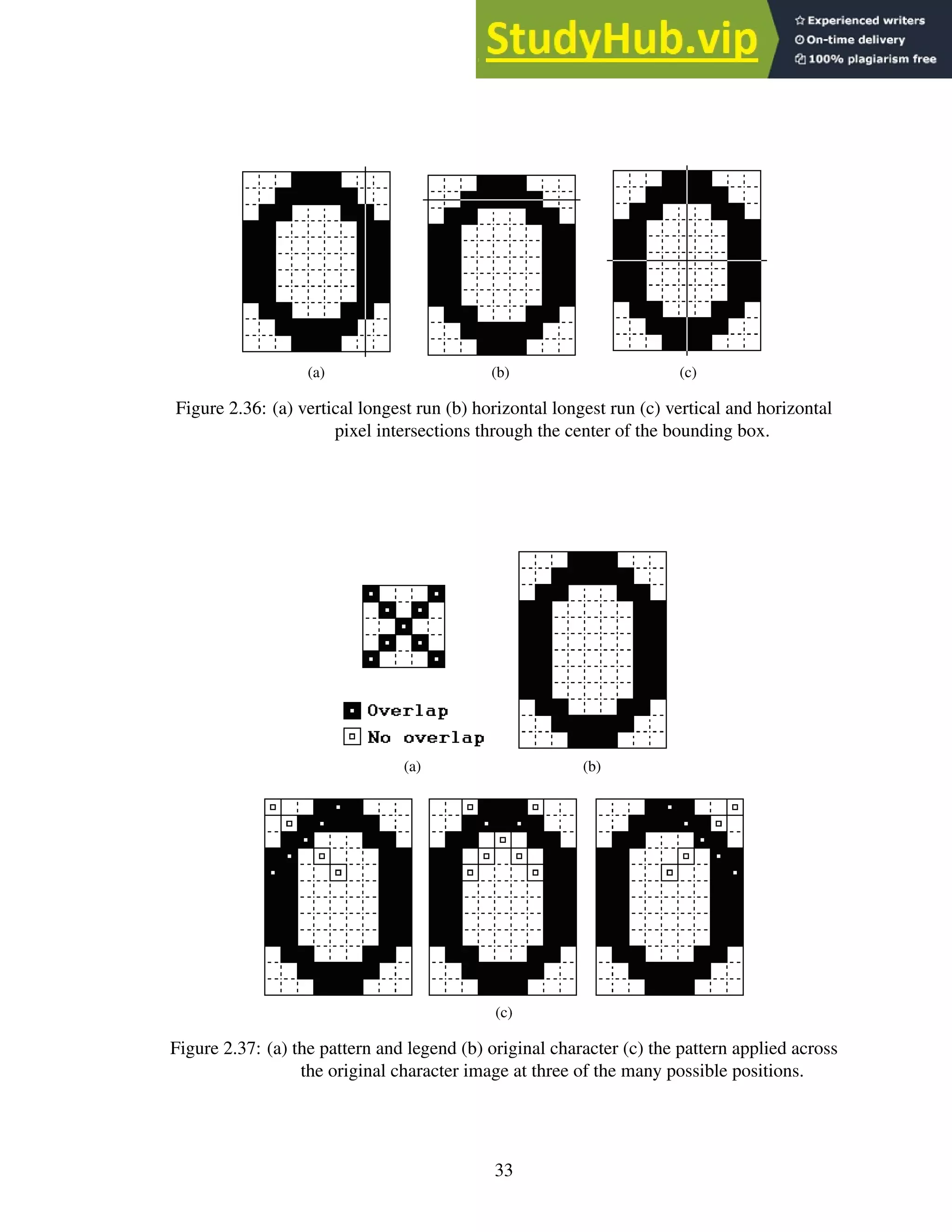
![counts the number of overlapping black pixels and uses these counts to identify the
glyph. For example, the vector generated by the first three overlays (as seen in Figure
2.37c) of the pattern shown in 2.37a to the character shown in 2.37b is {5, 2, 5}. These
values mean that the first overlay intersects 5 black pixels, the second intersects 2 pixels
and the last intersects 5 pixels. This method is useful because different patterns can
be implemented for different font sizes and styles, and the method works with non-
rectilinear bounding boxes.
(a) (b)
Figure 2.38: (a) three 72pt Arial characters overlayed on one another (b) filled locations
are unique to a single character.
I was unable to find any discussion on how to choose or design an appropriate pattern,
though I have an idea about how I might create one. For a given font size and style F,
a naïve approach creates a set of pixels P such that for each character in F, there exists
at least one overlapping pixel in P. Further, we create P so that a non-empty subset of P
uniquely identifies each character in F. For example, given the set of characters shown
in Figure 2.38, we can choose three pixels (one for each character) such that each pixel
both overlaps a character and uniquely identifies that character. The (x, y) coordinates of
these pixels form a pattern appropriate for disambiguating one character from another.
There are many variations on spatial-feature extraction techniques. The methods men-
tioned are just the basic types. The grid-and-count method can be extended to be pie-shaped
or have an arbitrary shape. The pattern-count method can be used with star-shaped patterns
or patterns that are designed by a genetic algorithm to determine their accuracy. There is
much room for research here. The best method is the one that best exploits the characteris-
tics of the specific alphabet or font set undergoing recognition.
Feature extraction: Transformational techniques
Transformational techniques convert the character image from a pixel representation to an-
other representation. Fourier and Wavelet transforms are examples of this type of technique
[48].
34](https://image.slidesharecdn.com/anopticalcharacterrecognitionengineforgraphicalprocessingunits-230805215723-24ac1bd2/75/An-Optical-Character-Recognition-Engine-For-Graphical-Processing-Units-47-2048.jpg)
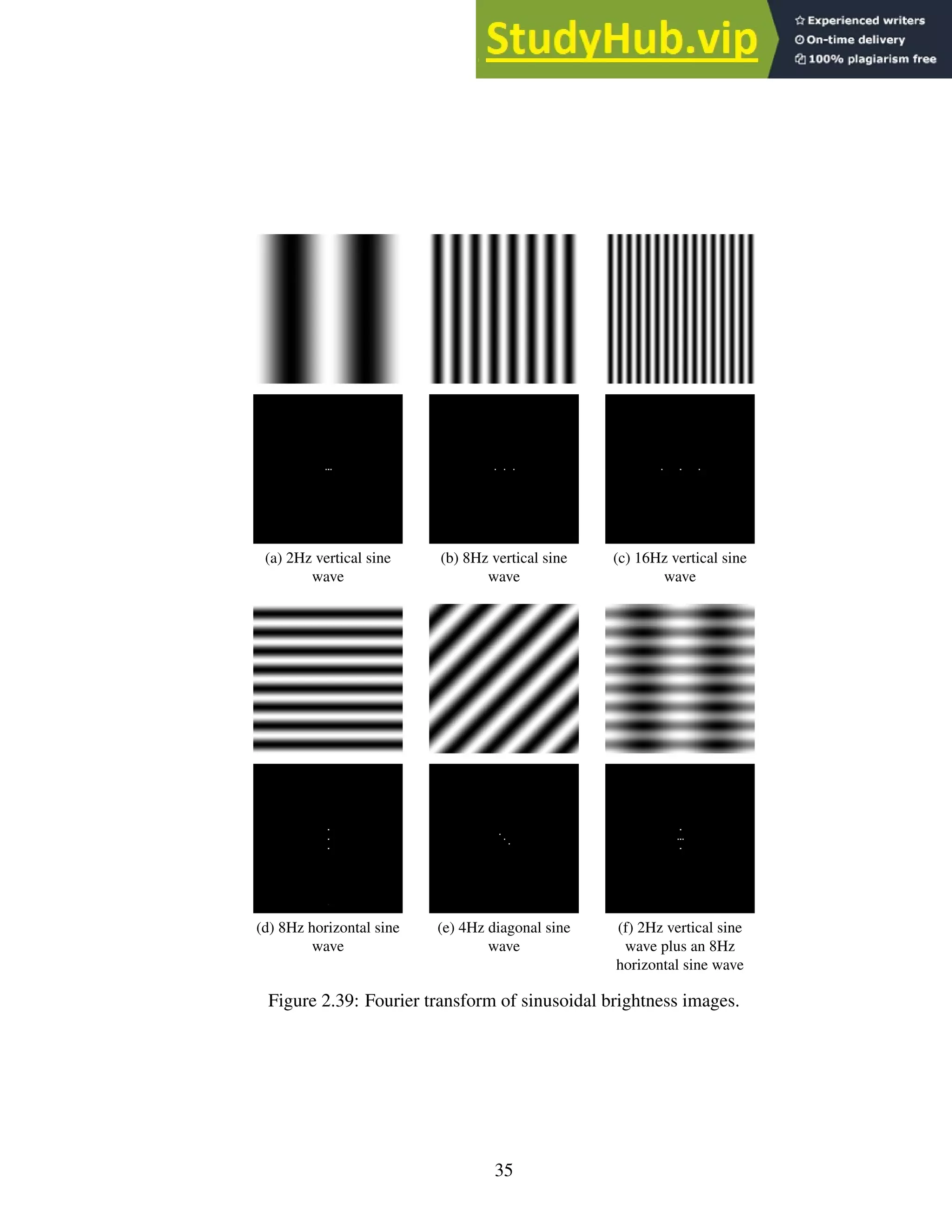
![1. The Fourier transform is generally used to analyze a closed planar curve. Since each
boundary on a character is a closed curve, the sequence of (x, y) coordinates that speci-
fies the curve is periodic, which makes conversion and analysis with a Fourier transform
possible [28, 30]. The discrete cosine transform is a variation of the Fourier transform.
(a) (b) (c)
Figure 2.40: Fourier transform of 3 character images.
The idea behind the Fourier transform is that any signal can be expressed as a sum
of a series of sine waves. In the case of images, the transform captures variations in
brightness across the image. Each wave, or sinusoid, in the series comprising the orig-
inal image is encoded in the output image of the transform by plotting the phase, the
frequency and the magnitude of the wave (the three variables necessary to describe a
sinusoid). Figure 2.39 on page 35 shows a series of brightness images corresponding to
various sine waves and their resultant Fourier transforms.
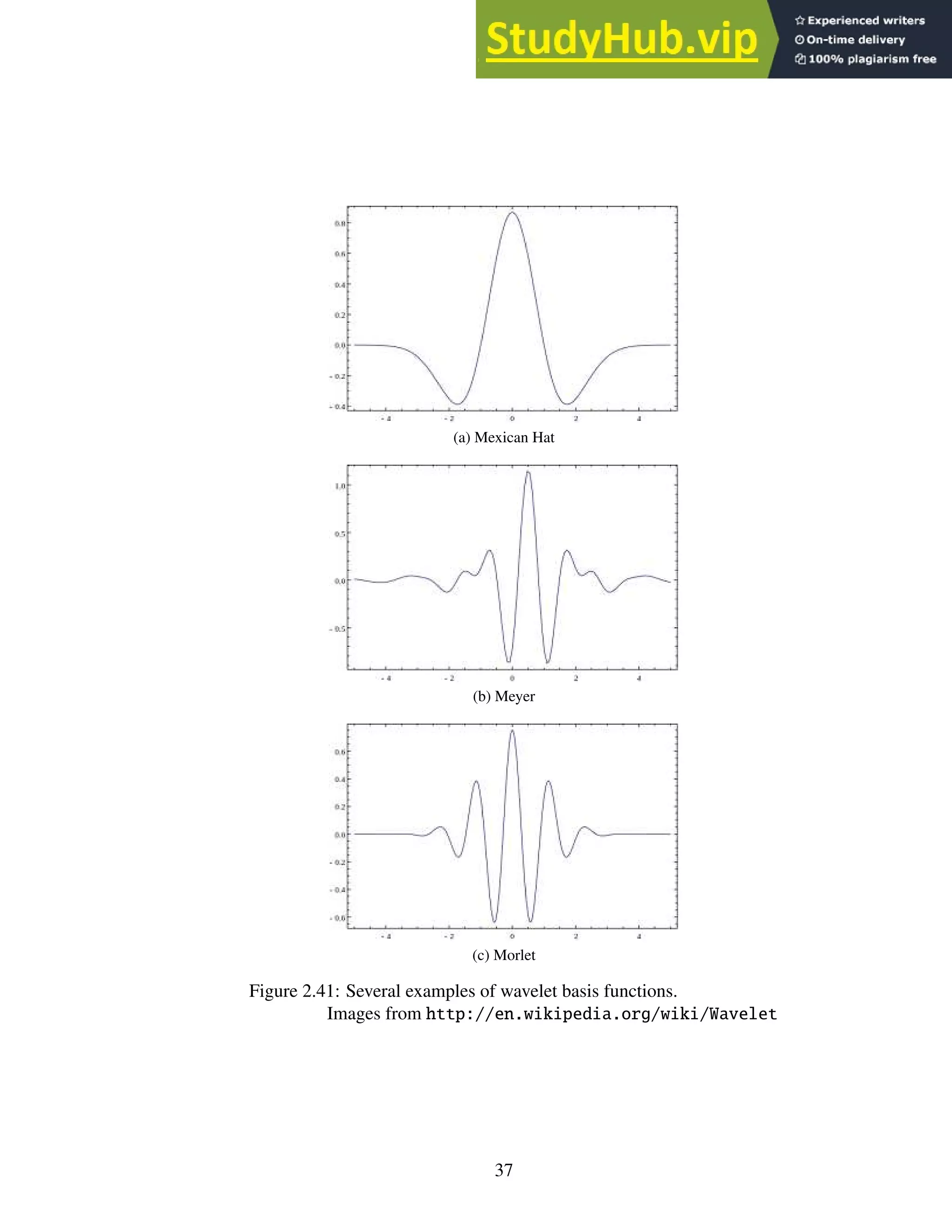
2. The main difference between a wavelet transform and a Fourier transform is the ba-
sis function upon which the transforms rely. Whereas Fourier transforms are limited
to the sine and cosine basis functions, the wavelet transform has no such limitation.
The absence of this limitation means that wavelet transforms can (and do) utilize wave
functions that have a defined beginning and end — that is, they are localized in space.
Wave functions that are localized in space are referred to as wavelets and is where the
transform gets its name [17]. See Figure 2.41.
To help clarify, I present an example using one of the basic wavelet basis functions,
called the Haar wavelet (see Figure 2.42). Suppose we are given an array of pixels,
representing a 1-d image:
[12, 4, 6, 10, 9, 2, 5, 7]
36](https://image.slidesharecdn.com/anopticalcharacterrecognitionengineforgraphicalprocessingunits-230805215723-24ac1bd2/75/An-Optical-Character-Recognition-Engine-For-Graphical-Processing-Units-49-2048.jpg)
![Figure 2.42: The Haar wavelet.
Image from http://en.wikipedia.org/wiki/Haar_wavelet
The Haar transform averages each pair of values (these are called data coefficients):
[12, 4, 6, 10, 9, 2, 5, 7] → [8, 8, 5.5, 6]
It then finds the difference between the maximum value in each original pair and its
average (these are called detail coefficients):
[8, 8, 5.5, 6] → [4, 2, 3.5, 1]
These two sets form the entire first run of the transform, which looks like:
[12, 4, 6, 10, 9, 2, 5, 7] → [8, 8, 5.5, 6, 4, 2, 3.5, 1]
The previous steps comprise one run of the Haar transform. Additional runs operate
recursively on the set of averages from the previous step. The detail coefficients do not
change and are copied through each run. When there is only one average left, no more
transforms can be computed. Thus, if the transform were to carry on for another run, the
result would look like:
[8, 8, 5.5, 6, 4, 2, 3.5, 1] → [8, 5.75, 0, .25, 4, 2, 3.5, 1]
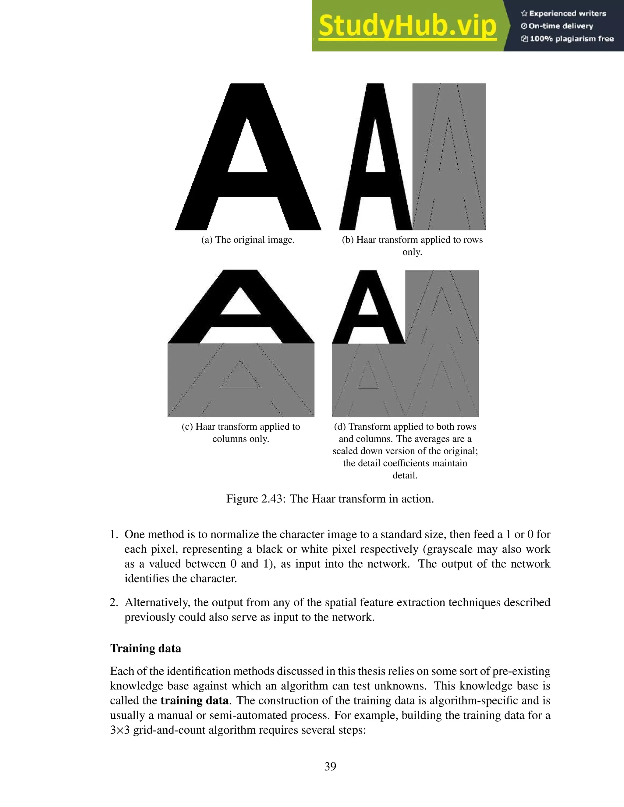
To generalize this approach to a 2-d image, the standard method is to apply the transform
to each pixel row of an image and then to each column [27, 54]. See Figure 2.43.
Feature extraction: Neural networks
A neural network does not explicitly extract features from a character image, rather, during
training, the network adjusts the internal pathway weights and connections within its neural
layers, indirectly molding itself to the features of a given pattern. This innate behavior of
the neural network, in essence, makes it a feature extraction technique, though it cannot
be easily classified as transformational or spatial. There are a myriad of ways to provide
image data to a neural network.
38](https://image.slidesharecdn.com/anopticalcharacterrecognitionengineforgraphicalprocessingunits-230805215723-24ac1bd2/75/An-Optical-Character-Recognition-Engine-For-Graphical-Processing-Units-51-2048.jpg)
![1. Find appropriate "training" glyph images
2. Pair each glyph image with its correct classification
3. Process each glyph image and store the results; these results comprise the training
data
Software can automate some of this process via embedding parts 2 and 3 in an interactive
program (i.e the software presents the user with a glyph image and the user provides the
classification). The software can also be configured to allow for manual correction of OCR
output [13].
2.9 Post-processing phase: Problems
This phase typically also includes the use of language-specific dictionaries and grammar
checks to help increase the overall accuracy of the OCR application.
Text reconstruction
During identification, the OCR application stores coordinates for each glyph (it can also
store other data, such as a confidence value for its classification and less-likely alternatives).
These coordinates correspond to the location of the glyph on the original image. During
text reconstruction, the OCR application sorts the glyphs based on these coordinates and
writes the characters to a text file. The difficulties lie in determining word boundaries and
spacing. Complex formats, such as double/triple column layouts, are typically ignored in
this stage and are not generally recreated.
Language-specific dictionaries and grammar checks
These post-processing techniques help increase the overall accuracy of the OCR application
by validating the reconstructed text.
1. Dictionary validation can help determine if a word should be “the” or “thc” when the
OCR engine could not.
2. If a word appears that is not in the dictionary and it contains a character from the con-
fusing character set, other characters from the set can be substituted to see if the word
becomes recognizable.
3. N-gram analysis provides another method to suggest possible corrections to a character
with a low-confidence value or a misspelled word. N-grams are sets of consecutive
items found in text or speech such as syllables, letters or words. For OCR, n-grams
are typically character sequences. A naïve use of this type of n-gram is to rank the
character sequences from most commonly found in a language, such as English, to least
commonly or never found in language. For example, the bigram "ou" is ranked higher,
or is more common, than the bigram "zz". Then, for misspelled words, low ranking
bigrams could be iteratively replaced with high ranking bigrams that contain one of
40](https://image.slidesharecdn.com/anopticalcharacterrecognitionengineforgraphicalprocessingunits-230805215723-24ac1bd2/75/An-Optical-Character-Recognition-Engine-For-Graphical-Processing-Units-53-2048.jpg)
![the original letters. The word can then be rechecked against the dictionary. I highly
recommend Kukich [25] for a full discussion on automatic word correction.
2.10 Conclusion
This chapter has presented a survey of both the problems that OCR engines must overcome
to recognize text and the techniques programmers and researchers implement to accomplish
the feat. I chose the selected references because they fulfill one of three purposes: the
reference provides a complete (or at least complete enough) description of the algorithm;
the reference provides an accessible introduction to a topic, or the reference is the seminal
paper on the topic. Additionally, I chose survey references over the original references
because they provide insight in comparing the algorithms and context for implementation.
41](https://image.slidesharecdn.com/anopticalcharacterrecognitionengineforgraphicalprocessingunits-230805215723-24ac1bd2/75/An-Optical-Character-Recognition-Engine-For-Graphical-Processing-Units-54-2048.jpg)
![1 // define kernel
2 __global__ void VectorAdd(float* A, float* B, float* C, int N)
3 {
4 int i = blockIdx.x * blockDim.x + threadIdx.x;
5 if (i < N)
6 C[i] = A[i] + B[i];
7 }
8
9 int main()
10 {
11 // define N as total input size
12 int N = ...;
13 size_t size = N * sizeof(float);
14
15 // allocate input vectors in host memory
16 float* host_A = (float*)malloc(size);
17 float* host_B = (float*)malloc(size);
18
19 // initialize input vectors
20 ...
21
22 // allocate vectors in GPU memory
23 float* GPU_A;
24 cudaMalloc(&GPU_A, size);
25 float* GPU_B;
26 cudaMalloc(&GPU_B, size);
27 float* GPU_C;
28 cudaMalloc(&GPU_C, size);
29
30 // copy vectors from host to GPU memory
31 cudaMemcpy(GPU_A, host_A, size, cudaMemcpyHostToDevice);
32 cudaMemcpy(GPU_B, host_B, size, cudaMemcpyHostToDevice);
33
34 // execute kernel
35 dim3 threadsPerBlock(256, 0, 0);
36 dim3 numBlocks((N + threadsPerBlock.x - 1) / threadsPerBlock.x, 0, 0);
37 VectorAdd<<<numBlocks, threadsPerBlock>>>(GPU_A, GPU_B, GPU_C, N);
38
39 // copy results from GPU memory to host memory
40 // GPU_C to host_C
41 cudaMemcpy(host_C, GPU_C, size, cudaMemcpyDeviceToHost);
42
43 // free GPU memory
44 cudaFree(GPU_A);
45 cudaFree(GPU_B);
46 cudaFree(GPU_C);
47
48 // free host memory, then manipulate the results
49 ...
50 }
Figure 3.2: Example CUDA program modified from the NVIDIA CUDA C Programming
Guide [34].
44](https://image.slidesharecdn.com/anopticalcharacterrecognitionengineforgraphicalprocessingunits-230805215723-24ac1bd2/75/An-Optical-Character-Recognition-Engine-For-Graphical-Processing-Units-57-2048.jpg)
![The threadsPerBlock and numBlocks variables define the grid size and shape for
the kernel. Both blocks and grids can be arbitrarily sized (with some restriction). However,
each GPU has limitations on the maximum number of threads in a block and the maximum
number of blocks in a grid. Current GPU devices limit the size of a block to 1536 threads
and a grid to 231
− 1 blocks.
Executing a kernel is the same as executing a function in C, except the dimensions of the
virtual grid and block constructs are specified between “<<<” and “>>>” using a variable
of type dim3, as shown in the example program in Figure 3.2.
3.4 GPU memory types
GPUs expose a variety of memory types with varying performance characteristics that a
programmer must take into account when designing a program for GPU. This section gives
a brief overview of the different types of GPU memory.
Register memory
Register memory is the fastest type of memory on a GPU. Variables declared in a kernel
are generally stored in a register, and each thread has its own copy of these variables.
However, the hardware limits each SM to 65,536 registers, and a single thread to 255
registers. If a kernel exceeds the hardware limit, the extra variables are stored in local
memory. Additionally, occupancy may be reduced by kernels using a large number of
registers. For example, if a kernel uses the maximum number of registers, a warp requires
8,160 registers, so that only 8 warps can be active at a time. Given 32 threads to a block, if
the SM has more than 8 cores, then occupancy is reduced. Register memory accesses occur
in less than one GPU clock cycle [10, 34].
Local memory
Local memory is the spill-over location for variables allocated in excess of hardware limi-
tations for registers. Local memory is actually a part of the global memory.
Shared memory
Shared memory comprises 65,536 bytes per SM. Because the shared memory is “on-chip”,
it has much lower access latency than other types of memory, except register memory. Al-
located shared memory is accessible by all threads in the same block and is often used for
communicating between threads. When a block finishes executing, it releases its shared
memory, which can then be re-allocated to other blocks. Like register memory, over-
allocating shared memory reduces occupancy. Shared memory accesses occur in approxi-
mately 22 GPU clock cycles [10, 34].
Constant memory
Constant memory has global scope and is available to all threads within a grid. Constant
memory shares the same performance characteristics as shared memory but is limited to
45](https://image.slidesharecdn.com/anopticalcharacterrecognitionengineforgraphicalprocessingunits-230805215723-24ac1bd2/75/An-Optical-Character-Recognition-Engine-For-Graphical-Processing-Units-58-2048.jpg)
![65,536 bytes [10, 34].
Texture memory
Texture memory is a read-only component of global memory accessed through dedicated
hardware optimized for read operations exhibiting high 2D spatial locality (i.e. reading
data elements close to one another). Texture memory is limited to the same size as global
memory minus allocations for padding and texture alignment. Texture memory has global
scope, is available to all threads within a grid and supports interpolated access [10, 34].
Global memory
Global memory is the largest, slowest type of memory on a GPU and is roughly 30× slower
than shared memory. Global memory is available to all threads within a grid. Global
memory accesses occur in approximately 600 GPU clock cycles [10, 34].
Why memory matters
The SegRec algorithm discussed in Chapter 4 is designed to process hundreds of page
images concurrently. I tested SegRec Version 3 with 1000 8.5”×11” page images at 200
dpi with ~1500 characters per page. SegRec must store the images and the output data for
~1.5 million characters. There must also be memory for each thread to process the images.
Memory allocation is critical for the speed of this algorithm.
Coalesced verses non-coalesced
GPU hardware tries to reduce memory reads and writes into as few transactions as pos-
sible. When a kernel takes advantage of this hardware characteristic by grouping reads
or writes into consecutive memory locations, it is called a coalesced read or a coalesced
write. Coalesced operations occur in the number of GPU clock cycles required for a sin-
gle operation of the same type. Non-coalesced operations are handled serially, with each
operation taking the full count of GPU clock cycles.
3.5 Programming hints
A programmer must observe several caveats when programming a GPU:
• On the device, each streaming multiprocessor (on current hardware) has up to 65,536
registers. All variables local to a kernel are stored in registers, which means these
registers must be split among all active threads on a SM. If you want a high occu-
pancy rate, the kernel must not contain a large number of local variables.
Fortunately, the compiler for CUDA reports how many registers the kernel uses. This
information allows the programmer to tweak the kernel in order to reduce the number
of registers needed.
46](https://image.slidesharecdn.com/anopticalcharacterrecognitionengineforgraphicalprocessingunits-230805215723-24ac1bd2/75/An-Optical-Character-Recognition-Engine-For-Graphical-Processing-Units-59-2048.jpg)
![• GPU memory is persistent between kernel executions, so unused memory should be
deallocated when the program no longer needs it. This persistence also means it is
possible to feed the results (or original data) from one kernel into another without
copying data between the host and the GPU.
• Copying data between the host and the GPU is typically the slowest step of a CUDA
program. If possible, one should compress the data or avoid copying altogether by
reusing earlier data.
• Registers are in short supply, but computation is cheap. Opt for recalculating over
storing a temporary result.
• Define blocks in multiples of 32 threads; otherwise the GPU adds “inactive threads”
to bring the block size up to the nearest multiple of 32, which can influence thread
ids.
• Warp divergence increases the overall execution time of the kernel. Use bit twid-
dling2
and if-conversion to avoid branching when applicable. See Appendix C on
page 92 for more information.
• There is limited support for recursion in NVIDIA GPU hardware architectures
≥ v2.0. However, stack space is allocated per-thread and must be pre-allocated.
Thus, memory allocation for recursive functions is difficult to predict and can be
wasteful. Given that memory is extremely limited on GPUs, recursion is generally
best avoided. Dynamic Parallelism (DP) is a viable alternative to recursion that is
supported in NVIDIA GPU architectures ≥ v3.5. DP allows “parent” grids to spawn
“child” grids without interacting with the host [34].
• There is no dynamic memory allocation within a kernel. A kernel cannot allocate
additional space during execution. However, shared memory can be dynamically
allocated when a kernel is first executed.
• Adding an “optimization” step that reduces occupancy may actually result in slower
execution than the original algorithm.
3.6 Conclusion
This chapter has presented a brief introduction into the virtual and physical architecture of
a graphical processing unit and the challenges in programming for such a device.
2
Bit Twiddling Hacks: http://graphics.stanford.edu/~seander/bithacks.html
47](https://image.slidesharecdn.com/anopticalcharacterrecognitionengineforgraphicalprocessingunits-230805215723-24ac1bd2/75/An-Optical-Character-Recognition-Engine-For-Graphical-Processing-Units-60-2048.jpg)
![Figure 4.1: A graphical representation of Version 1 of the SegRec algorithm.
form a bounding box for the glyph. The output of this step is a list of bounding boxes
corresponding to the glyphs in each line.
The next stage removes completely white rows from each bounding box, shrinking the
box to be as compact as possible. This stage counts pixels on the rows within the glyph
bounding box and removes rows with zero black pixels. The output of this step is a list of
best-fit bounding boxes corresponding to the glyphs in each line.
In order to recognize each glyph, the next stage partitions each bounding box into a
5×5 grid, counts the number of black pixels in each region within the grid and computes a
25-dimensional vector containing the counts.
Figure 4.2 shows a 3×3 grid, but the idea is the same. Starting from the bottom-left,
counting the black pixels in each region results in the following 9-dimensional vector:
(13, 1, 15, 7, 9, 11, 3, 18, 7)
By dividing each element of the vector by the total area of the glyph, the algorithm
calculates the Global Density Vector (GDV) for the glyph:
(.034, .002, .039, .018, .024, .029, .008, .047, .018)
Version 1 finds the closest match in Euclidean 25-space for this GDV within the training
data; the character associated with that match is the recognized character. The search is a
brute-force comparison of the distance between the search vector against all the vectors in
the training data. A more efficient method is the k-d tree nearest-neighbor search, but this
search requires recursion, which has only limited support on GPUs [13].
The main flaw in this algorithm is that it can only operate on characters cleanly sep-
arated by white space. Due to the way the algorithm forms bounding boxes, at least one
49](https://image.slidesharecdn.com/anopticalcharacterrecognitionengineforgraphicalprocessingunits-230805215723-24ac1bd2/75/An-Optical-Character-Recognition-Engine-For-Graphical-Processing-Units-62-2048.jpg)
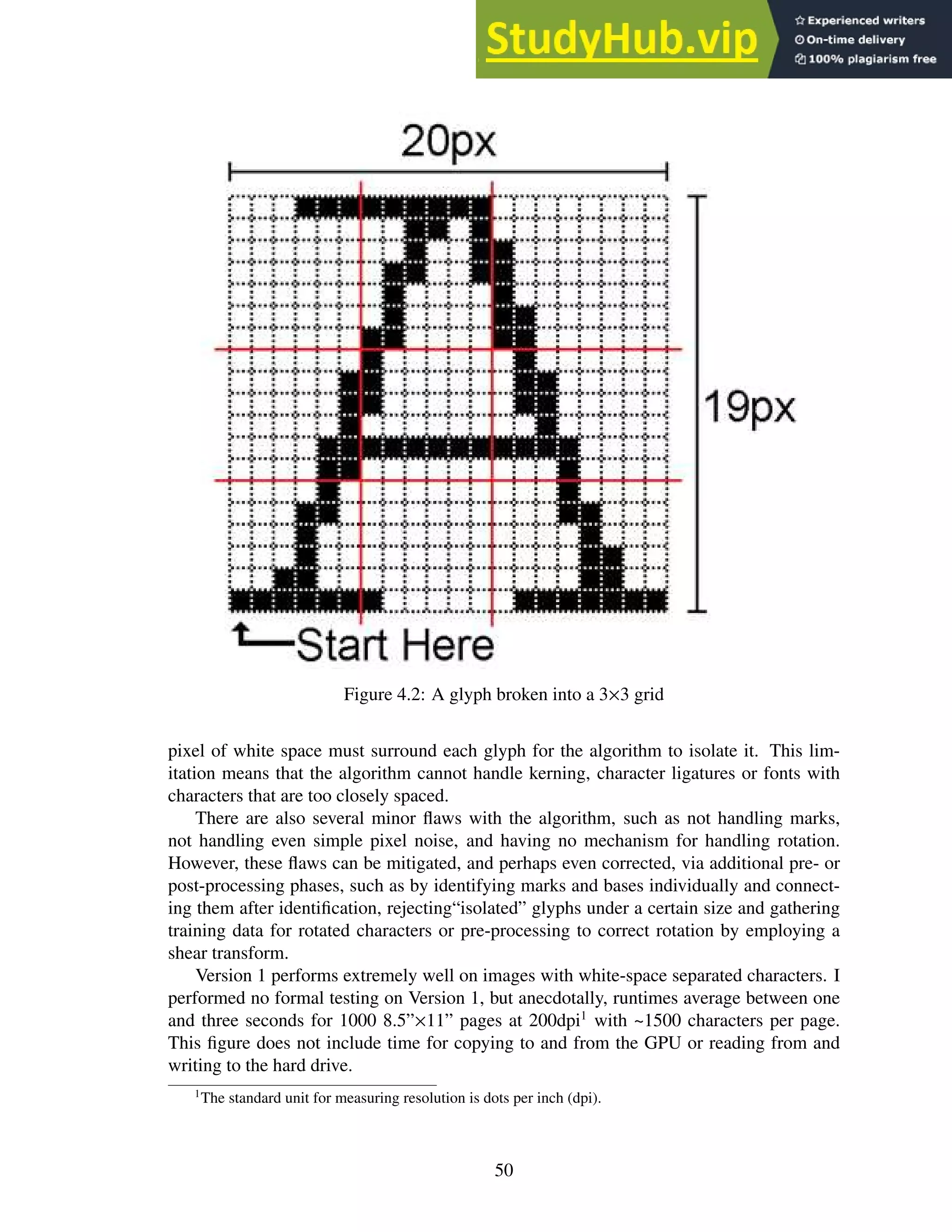
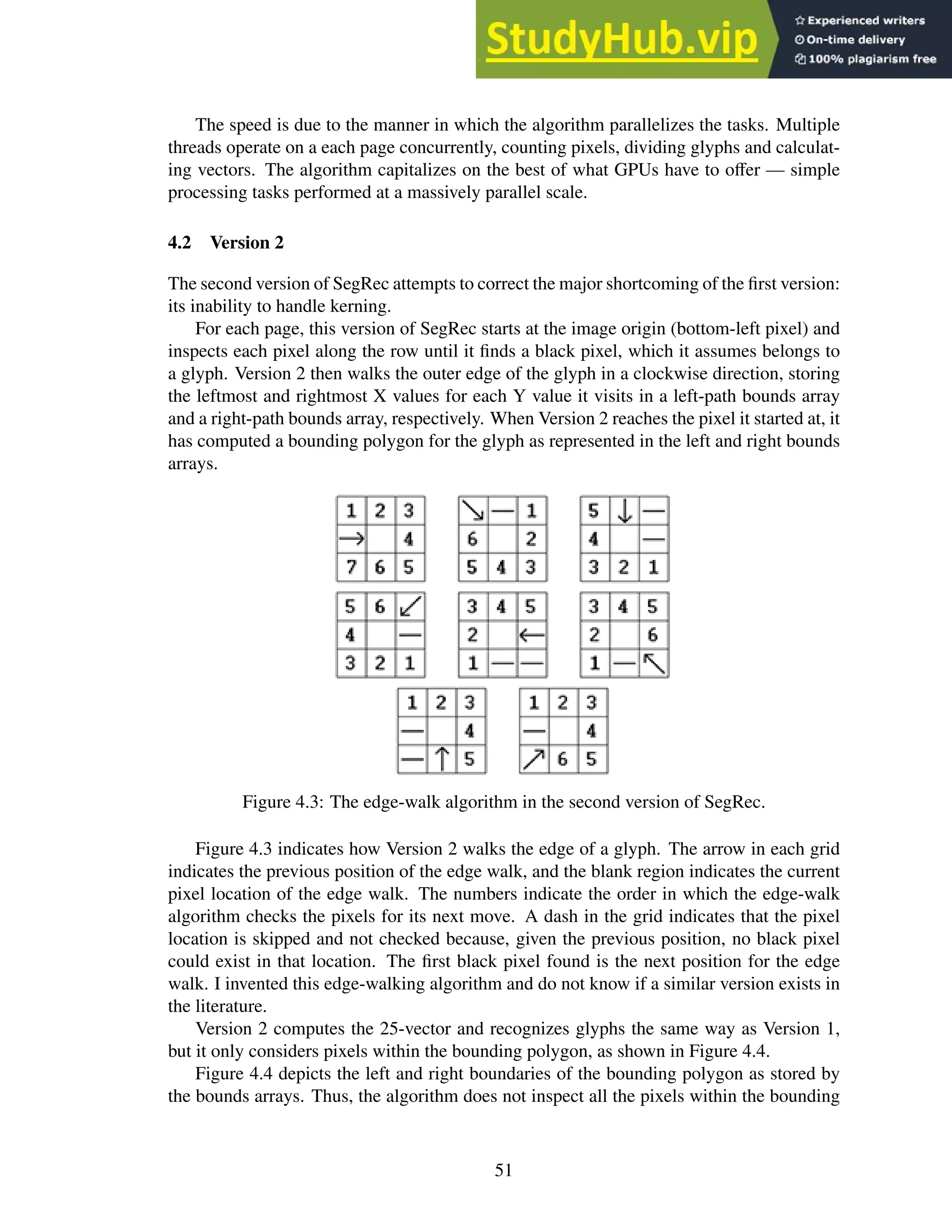
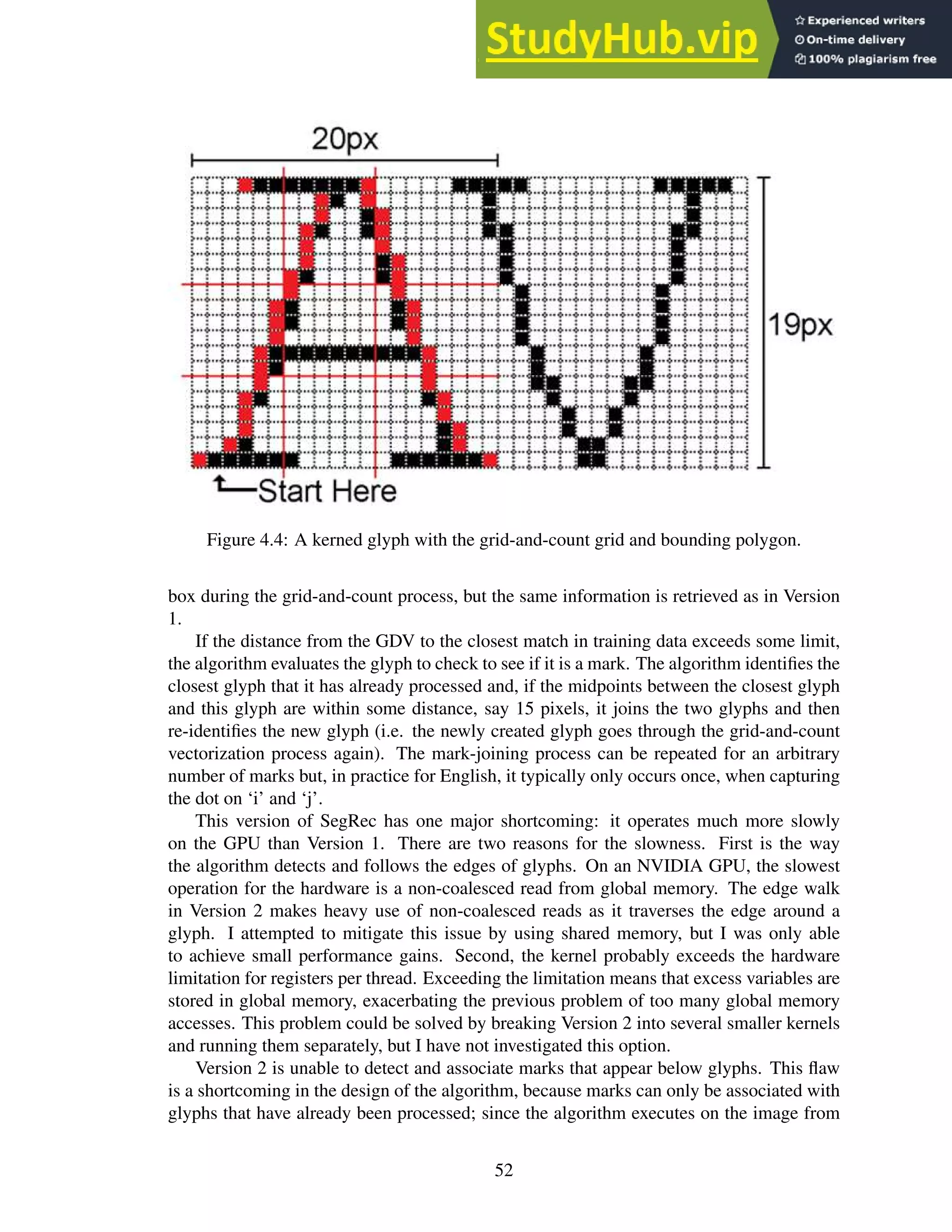
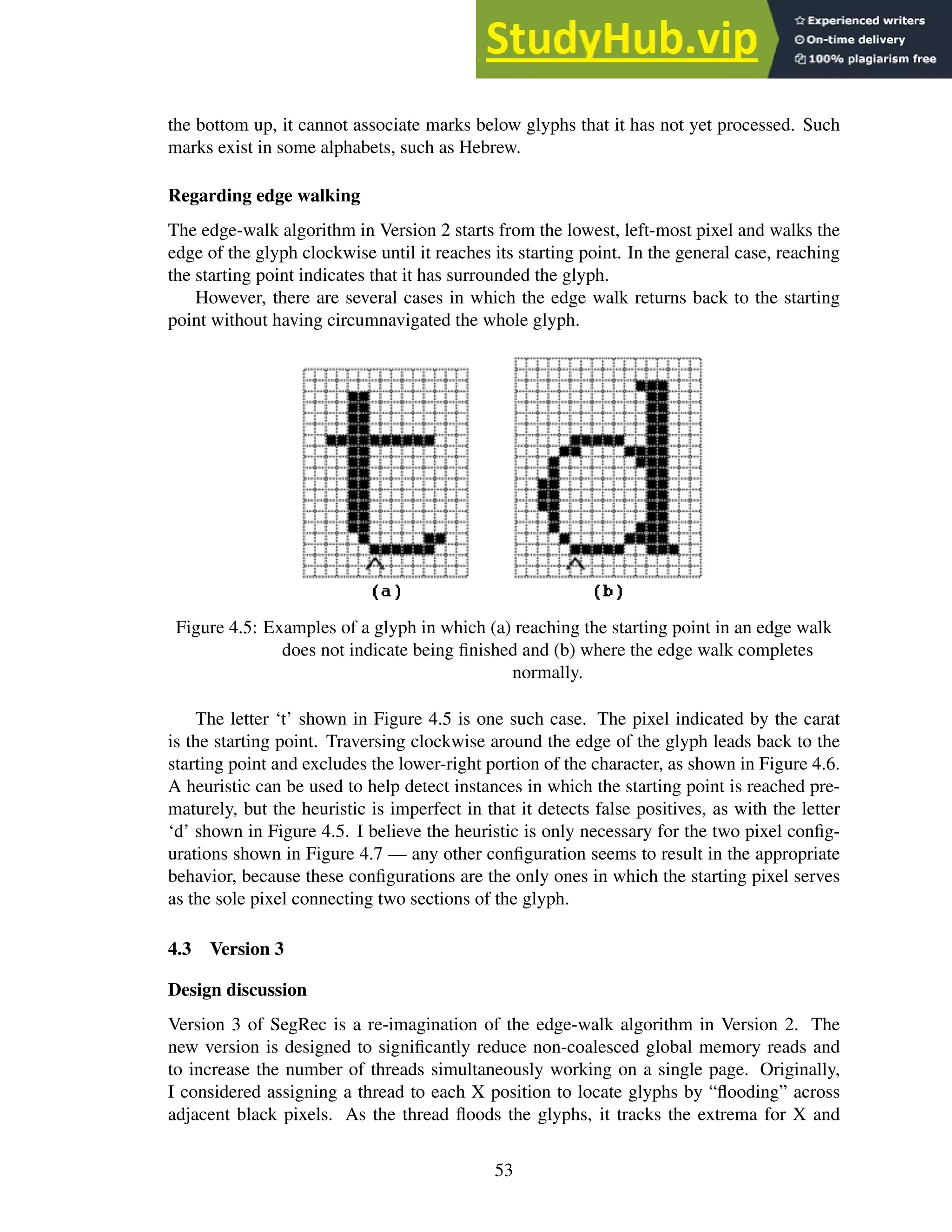
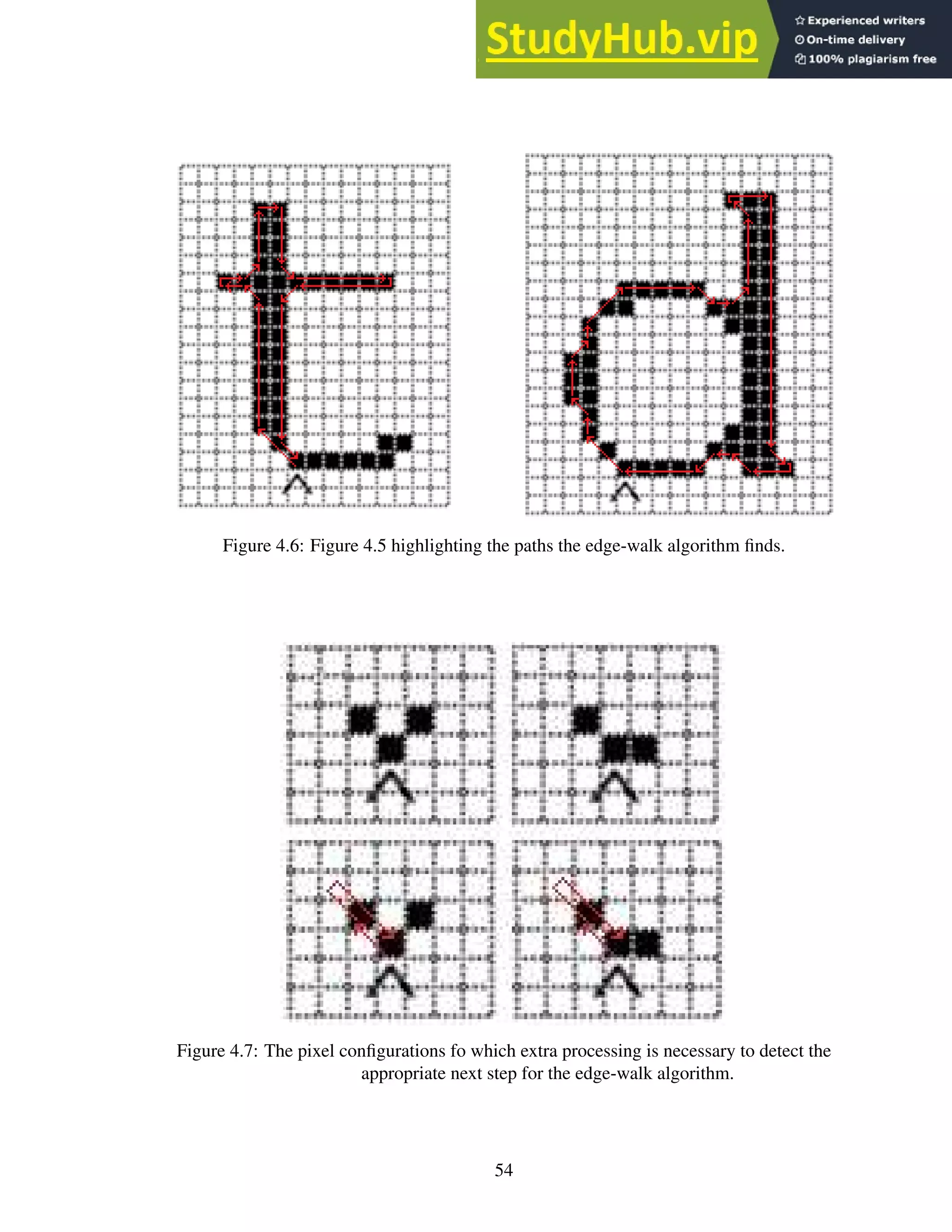
![Y and calculates a bounding box for the glyph. However, the threads would constantly
be overwriting each other and duplicating work as several of them would be operating on
the same glyph. In order to overcome this limitation, the threads could potentially replace
black pixels with their ThreadID and have the highest ThreadID “win”. Thus, if a thread
were to check a pixel and find a ThreadID higher than its own, the thread would move to
other work. However, this algorithm would require the storage for images to jump from 1
bit per pixel to 16 bits per pixel (in order to accommodate storing the ThreadID), which
would exceed the memory capabilities of many GPUs. Additionally, there is no way to
intelligently allocate memory for output from each of the threads. Because there is no way
to pre-determine which thread will “win” each glyph, a huge excess of memory must be
allocated for each thread, again, potentially exceeding the memory capabilities of many
GPUs.
The next idea was to reduce the thread count to a maximum of 255 per image. This
approach would only increase the input image size from 1 bit per pixel to 8 bits per pixel
instead of 16 bits per pixel. However, it still does not solve the issue of allocating storage
space for thread output, since there is still no way to pre-determine “winners”.
At this point, I shifted focus to exactly what the algorithm would output. Initially, the
algorithm was supposed to output the left and right boundaries associated with each glyph.
However, assuming 100 boundary values per glyph, which gives us a maximum height of
50 pixels (50 boundary values for the left path and 50 values for the right path) at 64 bits
per coordinate (32 bits each for X and Y) and a target throughput of 2.5 million characters,
the required storage equals ~2GB — too much memory to use for output.2
At this point, I
discarded the idea of storing and outputting the full paths. Next, I considered the possibility
of storing a path approximation.
The DPHull algorithm is a variation and improvement upon the Douglas-Peucker line-
simplification algorithm [18]. DPHull reduces the number of vertices that comprise a
closed polygon by incrementally adjusting the position of existing vertices to remove in-
termediate vertices. Applying DPHull has the effect of slightly altering the shape of the
polygon approximation. DPHull sets a threshold for the difference and only allows cumu-
lative changes that fall under the threshold. For a glyph, the difference can be relatively
large (even up to several pixels on both sides of the glyph) while still capturing the overall
shape within a reduced set of coordinates.
However, the paths need not even be stored at all. Since the eventual goal is to compute
the 25-space vector to classify the glyph, we can simply store the path temporarily in order
to compute the vector. The same logic could be applied to the vector, but I choose to output
it, in addition to the other glyph data: bounding box coordinates and the proposed character
classification.
This line of inquiry and realization led to the creation of Version 3.
2
32 bits were required because SegRec stacks the images, thus, for 1000 pages, the y-value ranges from 0
to 2,199,999. Later, I figured out I could use 32 bits for each boundary value (16 bits per component) because
the page offset is calculable and the height of a page is constant.
55](https://image.slidesharecdn.com/anopticalcharacterrecognitionengineforgraphicalprocessingunits-230805215723-24ac1bd2/75/An-Optical-Character-Recognition-Engine-For-Graphical-Processing-Units-68-2048.jpg)
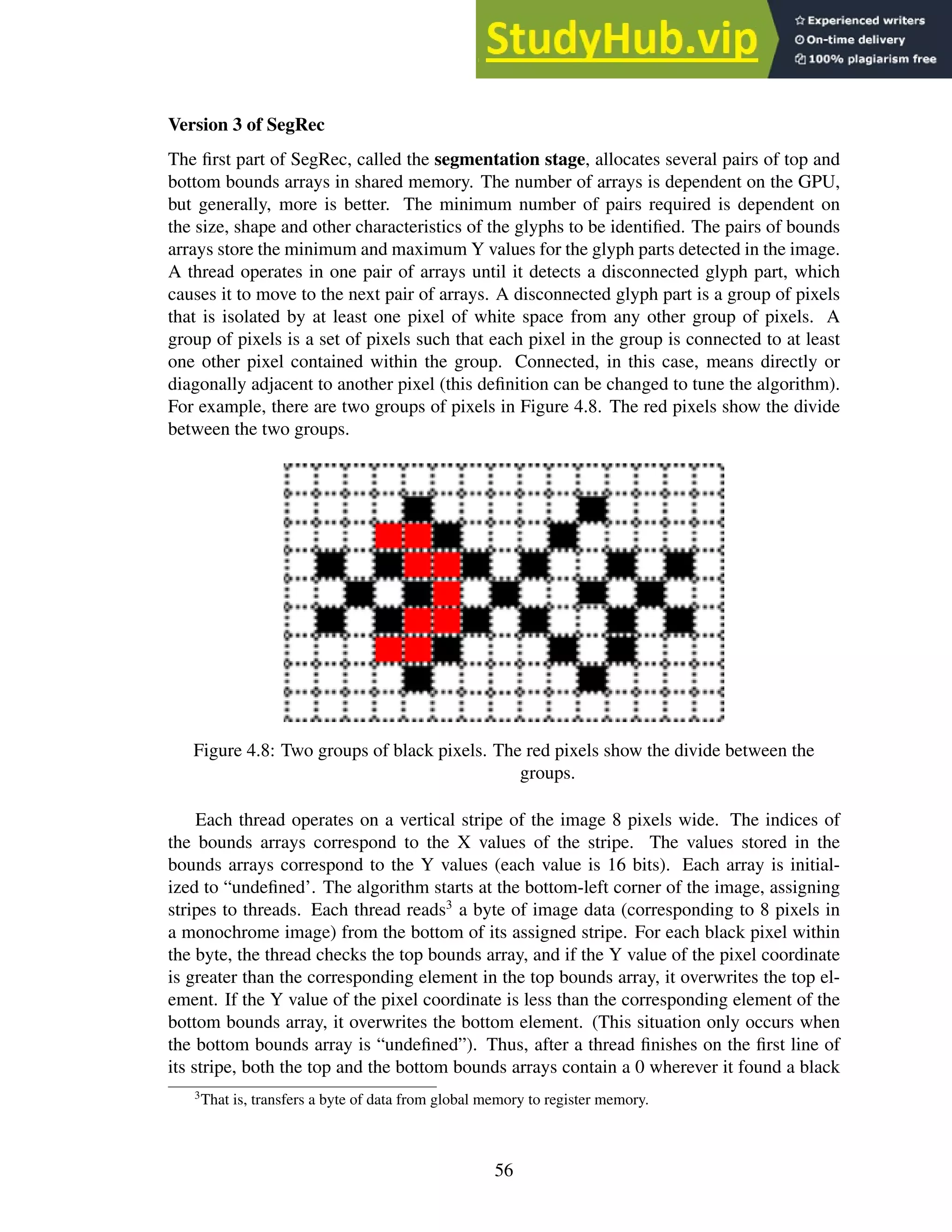
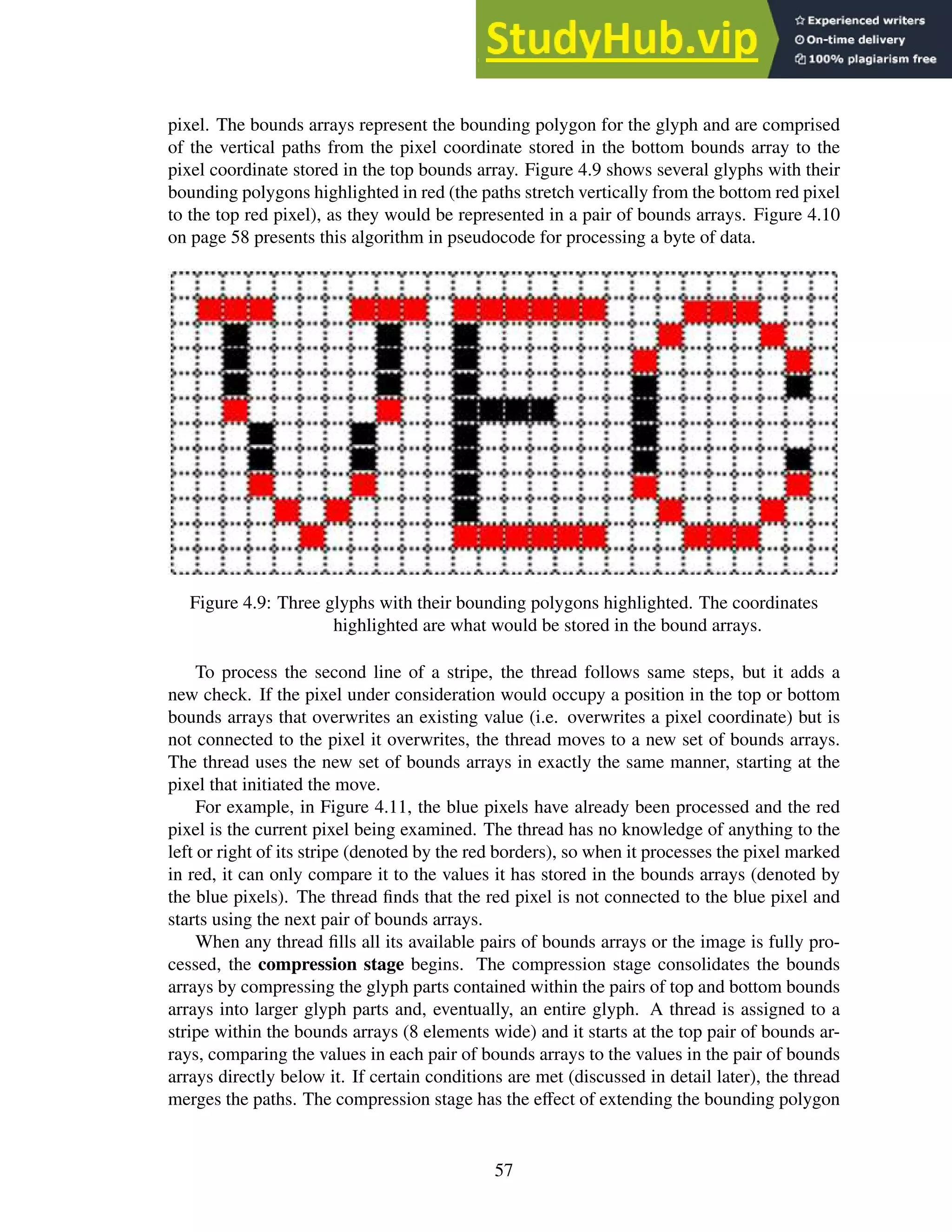
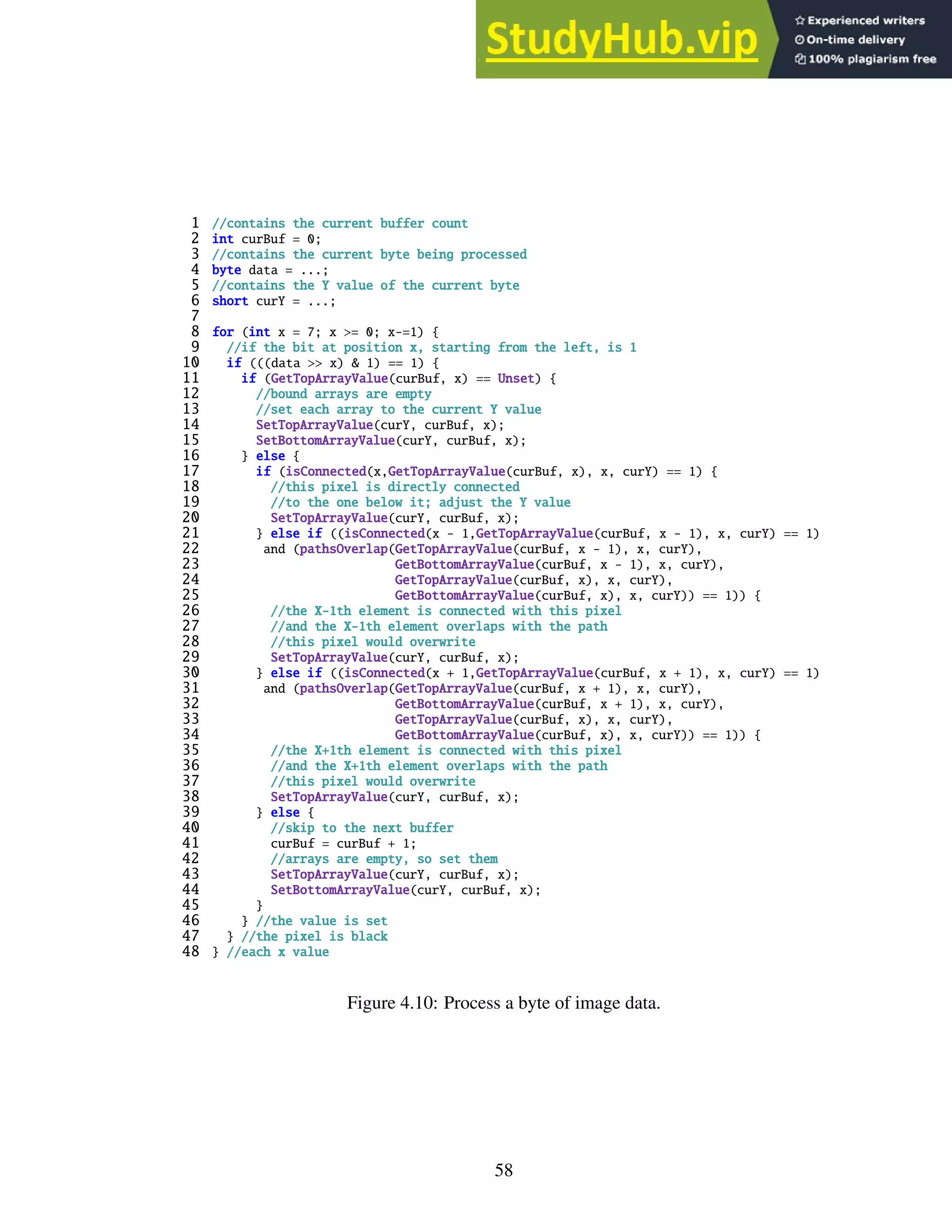
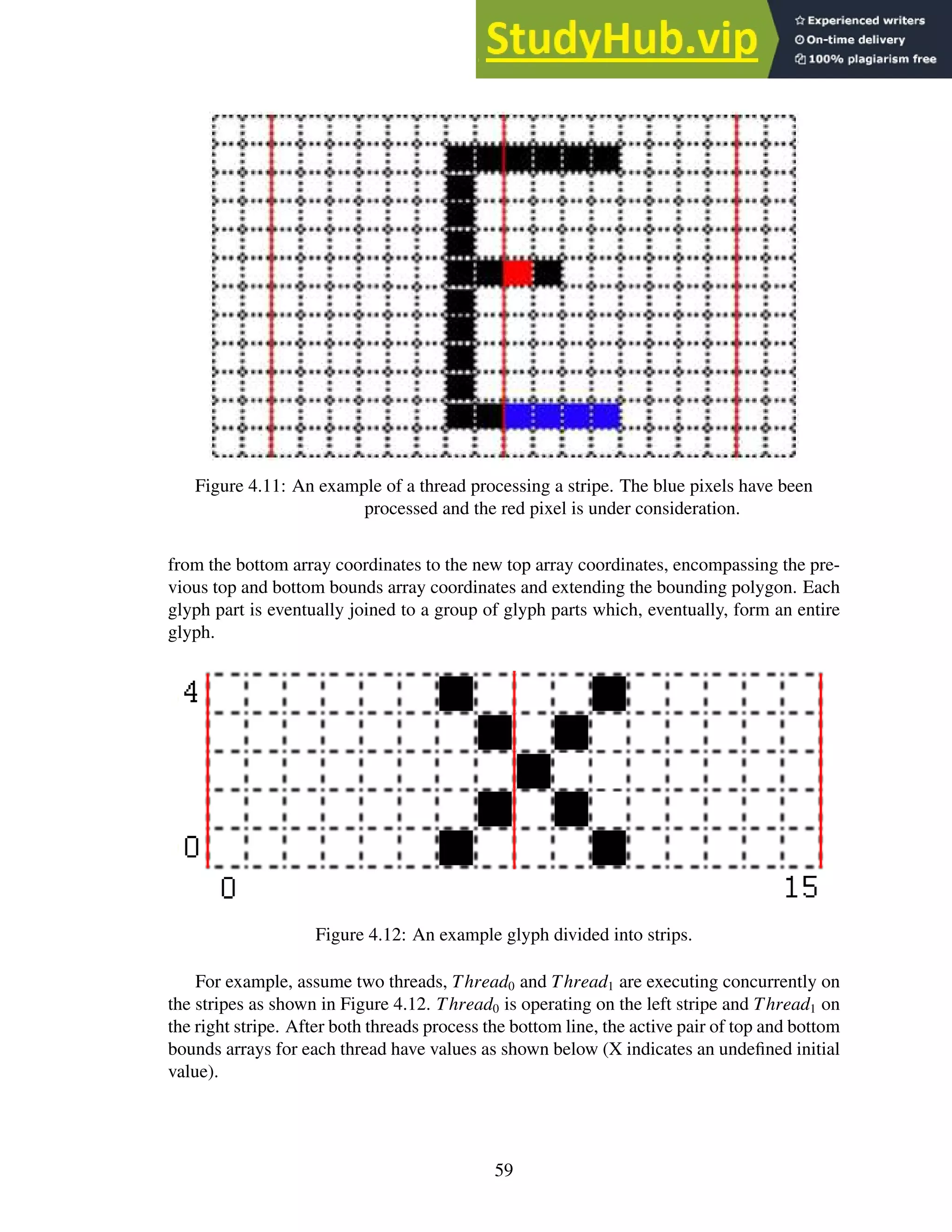
![A fter line 0 :
Top0 : [X,X,X,X,X,X,0,X] [X,X,0,X,X,X,X,X]
Bottom0 : [X,X,X,X,X,X,0,X] [X,X,0,X,X,X,X,X]
The bounds arrays show that Thread0 sees a black pixel at (6, 0) and Thread1 sees a
black pixel at (10, 0). Because these pixels overwrite an unset element, they do not need to
be connected to any previous entries.
A fter line 1 :
Top0 : [X,X,X,X,X,X,0,1] [X,1,0,X,X,X,X,X]
Bottom0 : [X,X,X,X,X,X,0,1] [X,1,0,X,X,X,X,X]
The threads add an additional pixel to the bounds arrays at (7, 1) and (9, 1), respectively.
Both of these pixels overwrite an unset element, so they do not need to be connected (even
though: (7, 1) is connected to (6, 0) and (9, 1) is connected to (10, 0)).
A fter line 2 :
Top0 : [X,X,X,X,X,X,0,1] [2,1,0,X,X,X,X,X]
Bottom0 : [X,X,X,X,X,X,0,1] [2,1,0,X,X,X,X,X]
Thread0 sees only white pixels in line 2, so it does not modify any values in the bounds
arrays. Thread1 sees an additional pixel at (8, 2). This pixel overwrites an unset element,
so it does not need to be connected (even though it is: (8, 2) is connected to (9, 1)).
A fter line 3 :
Top1 : [X,X,X,X,X,X,X,3] [X,X,X,X,X,X,X,X]
Bottom1 : [X,X,X,X,X,X,X,3] [X,X,X,X,X,X,X,X]
Top0 : [X,X,X,X,X,X,0,1] [2,3,0,X,X,X,X,X]
Bottom0 : [X,X,X,X,X,X,0,1] [2,1,0,X,X,X,X,X]
Thread0 sees a pixel at (7, 3), but because the pixel is not connected to any existing
coordinate stored in first set of bounds arrays (the algorithm checks the X − 1th and Xth
element for connectedness), the thread starts using the next pair of bounds arrays. Thread0
adds (7, 3) to the new pair of bounds arrays. Thread1 continues to use the first pair of
bounds arrays and adds an additional pixel found at (9, 3). Because (9, 3) overwrites an
existing pixel coordinate, the thread verifies that it is connected: (9, 3) is connected to
(8, 2).
60](https://image.slidesharecdn.com/anopticalcharacterrecognitionengineforgraphicalprocessingunits-230805215723-24ac1bd2/75/An-Optical-Character-Recognition-Engine-For-Graphical-Processing-Units-73-2048.jpg)
![A fter line 4 :
Top1 : [X,X,X,X,X,X,4,3] [X,X,X,X,X,X,X,X]
Bottom1 : [X,X,X,X,X,X,4,3] [X,X,X,X,X,X,X,X]
Top0 : [X,X,X,X,X,X,0,1] [2,3,4,X,X,X,X,X]
Bottom0 : [X X,X,X,X,X,0,1] [2,1,0,X,X,X,X,X]
Thread0 sees a pixel at (6, 4) and adds it to its current pair of bounds arrays. Thread1
sees a pixel at (10, 4). Both pixels overwrite existing coordinates; and the threads verify
that they are connected. (6, 4) is connected to (7, 3) in the second set of bounds arrays and
(10, 4) is connected to (9, 3).
For the sake of the example, say that both threads have completed their entire stripes.
The bounds arrays now represent a polygonal bounding box around the glyph, as shown in
Figure 4.13. Each color represents a different pair of bounds arrays — the blue pixels show
paths stored by S 0, a thread’s first pair of bounds arrays, and the red pixels show paths
stored by S 1, a thread’s second pair of bounds arrays. The compression stage now begins.
Figure 4.13: A glyph encircled by a polygonal bounding box.
I use the following conventions to refer to the pairs of bounds arrays, the positions
within them and the coordinates they represent:
• S n indicates the concatenation of the nth pair of bound arrays across all threads; i.e.
S 0 is the first pair, S 1 is the second pair and so on.
• S n[T|B|A] refers to the top, bottom or both (all) bounds arrays in pair, S n; i.e. S 0B
refers to the bottom bounds array in the first pair and S 1T refers to the top bound
array in the second pair. S 1A refers to both the top and bottom bound arrays in the
second pair.
• S n[T|B|A]m indicates stripe m in the [T|B|A] bounds array in pair S n; i.e. S 0B0 is the
first stripe in the bottom array in the first pair of bounds arrays. In this example, a
stripe consists of eight indices (corresponding to the 8 pixels within the stripes on the
image).
61](https://image.slidesharecdn.com/anopticalcharacterrecognitionengineforgraphicalprocessingunits-230805215723-24ac1bd2/75/An-Optical-Character-Recognition-Engine-For-Graphical-Processing-Units-74-2048.jpg)
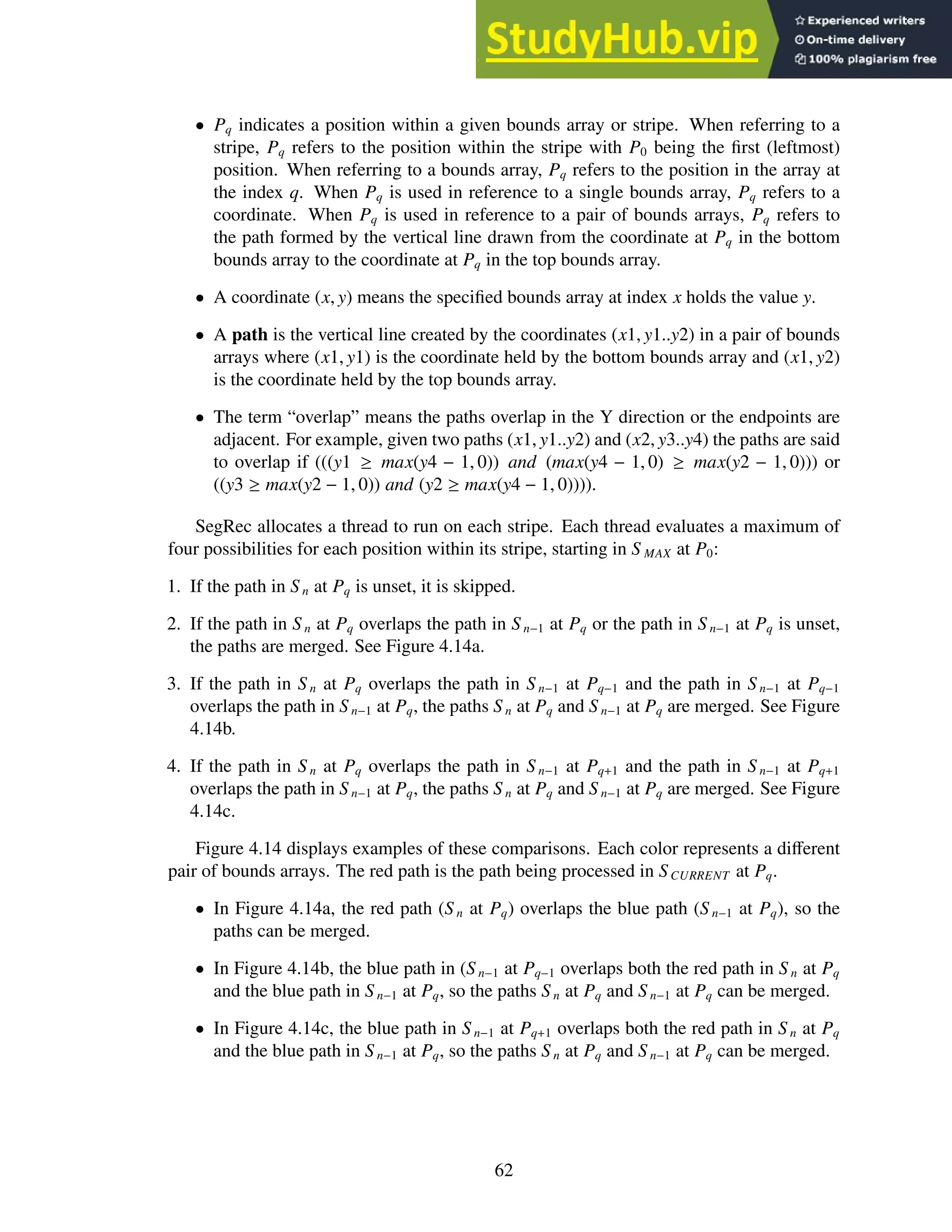
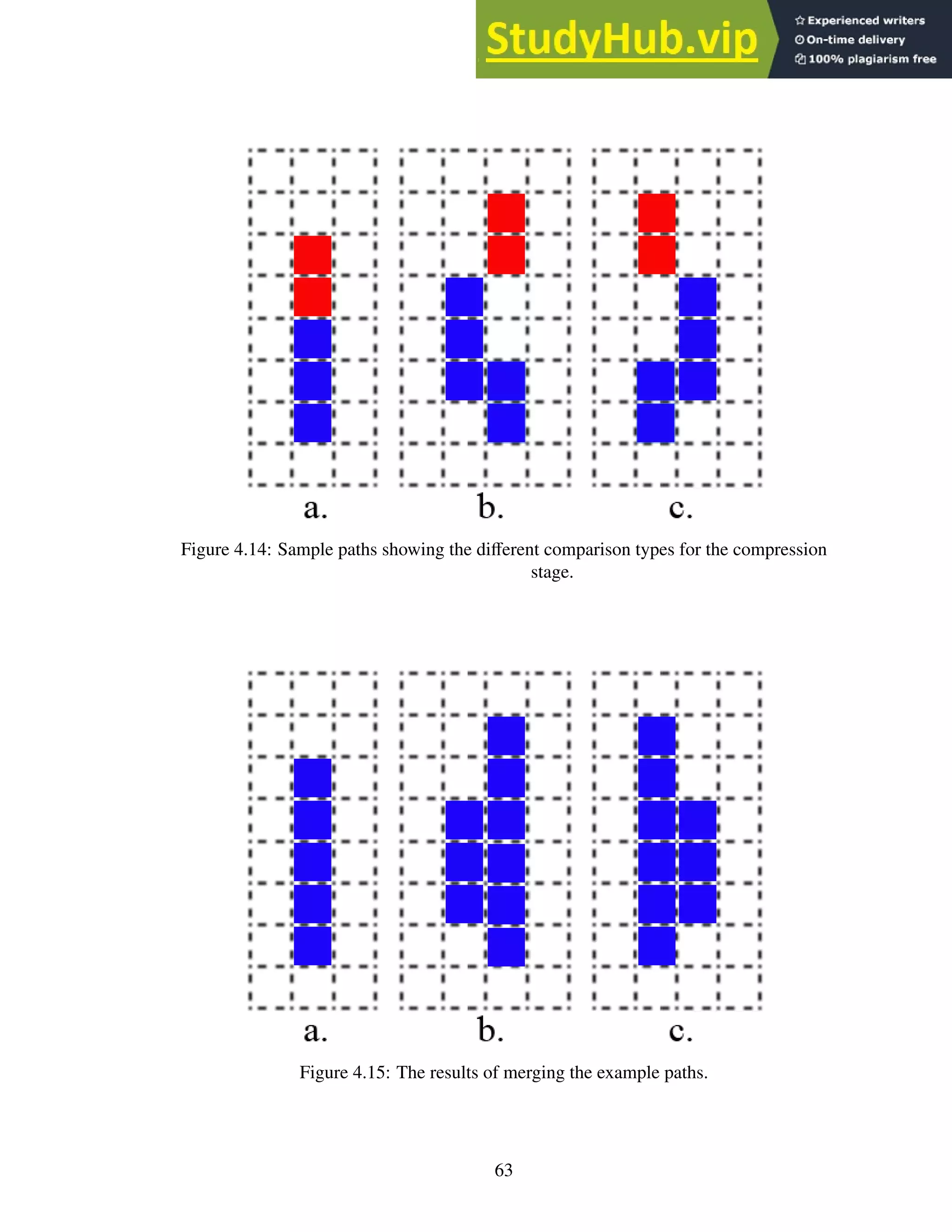
![Merging combines the paths by moving the value in S nT at Pq to S n−1T at Pq, overwrit-
ing the previous value. If the path in S n−1 is unset, the value in S nB at Pq is also moved.
Merging the paths extends the boundaries of the polygonal bounding box from the bottom
of the path in S n−1 at Pq to the top of the path in S n at Pq, as seen in Figure 4.15.
From the example in Figure 4.13, the bounds arrays currently appear as follows:
S tart state :
Top1 : [X,X,X,X,X,X,4,3] [X,X,X,X,X,X,X,X ]
Bottom1 : [X,X,X,X,X,X,4,3] [X,X,X,X,X,X,X,X ]
Top0 : [X,X,X,X,X,X,0,1] [2,3,4,X,X,X,X,X ]
Bottom0 : [X,X,X,X,X,X,0,1] [2,1,0,X,X,X,X,X ]
SegRec allocates two threads, Thread0 and Thread1 to operate on the two stripes.
Thread0 processes the left stripe and Thread1 processes the right stripe. Thread0 skips
the unset positions and arrives at P6. Thread0 compares S1 at P6 to S 0 at P6 and finds the
paths do not overlap. Thread0 then compares S1 at P6 to S0 at P5 and finds the paths do
not overlap. Thread0 then compares S 1 at P6 to S 0 at P7 and finds the paths do not overlap.
Thread0 is done processing P6 in S 1. Thread1 finds only unset positions and skips them
all.
Thread0 arrives at P7. Thread0 compares S 1 at P7 to S 0 at P7 and finds the paths do
not overlap. Thread0 then compares S 1 at P7 to S 0 at P6 and finds the paths do not overlap.
Thread0 then compares S 1 at P7 to S 0 at P8 (which crosses the stripe border) and finds the
paths overlap. Thread0 then compares S0 at P7 to S 0 at P8 and finds the paths overlap.
Thread0 then merges P7 in S 1 to P7 in S 0. Thread0 unsets P7 in S 1.
A fter pass 1 :
Top1 : [X,X,X,X,X,X,4,X] [X,X,X,X,X,X,X,X]
Bottom1 : [X,X,X,X,X,X,4,X] [X,X,X,X,X,X,X,X]
Top0 : [X,X,X,X,X,X,0,3] [2,3,4,X,X,X,X,X]
Bottom0 : [X,X,X,X,X,X,0,1] [2,1,0,X,X,X,X,X]
Since Thread0 has made a change, all threads perform another compression pass. The
threads repeat this process until no thread makes a change.
Thread0 skips all the unset positions and arrives at P6. Thread0 compares S 1 at P6 to
S 0 at P6 and finds the paths do not overlap. Thread0 then compares S 1 at P6 to S 0 at P5
and finds the paths do not overlap. Thread0 then compares S 1 at P6 to S 0 at P7 and finds
the paths overlap. Thread0 then compares S 0 at P7 to S 0 at P6 and finds the paths overlap.
Thread0 then merges P6 in S 1 to P6 in S 0. Thread0 unsets P6 in S 1. Thread0 skips P7,
because it is unset. Thread1 finds only unset positions and skips them all.
64](https://image.slidesharecdn.com/anopticalcharacterrecognitionengineforgraphicalprocessingunits-230805215723-24ac1bd2/75/An-Optical-Character-Recognition-Engine-For-Graphical-Processing-Units-77-2048.jpg)
![A fter pass 2 :
Top1 : [X,X,X,X,X,X,X,X] [X,X,X,X,X,X,X,X]
Bottom1 : [X,X,X,X,X,X,X,X] [X,X,X,X,X,X,X,X]
Top0 : [X,X,X,X,X,X,4,3] [2,3,4,X,X,X,X,X]
Bottom0 : [X,X,X,X,X,X,0,1] [2,1,0,X,X,X,X,X]
Since Thread0 has again made a change, all threads perform another compression pass.
Pass 3 results in no changes, so the compression stage is complete. Figure 4.16 shows the
final bounding polygon for this example.
A fter pass 3 :
Top1 : [X,X,X,X,X,X,X,X] [X,X,X,X,X,X,X,X]
Bottom1 : [X,X,X,X,X,X,X,X] [X,X,X,X,X,X,X,X]
Top0 : [X,X,X,X,X,X,4,3] [2,3,4,X,X,X,X,X]
Bottom0 : [X,X,X,X,X,X,0,1] [2,1,0,X,X,X,X,X]
Figure 4.16: The bounding polygon for the example.
Version 3 of SegRec processes all stripes concurrently due to the mechanism by which
the threads operate on the GPU, assuming we only use one warp per page. Each thread
within a warp executes the same instructions at the same time; thus, each thread is at
exactly the same point within the compression stage at the same time, so there is no chance
the threads can directly interfere with one another. However, it is possible that a thread
could run out of bounds arrays before it, or some other thread, has seen the full glyph.
Thus, Version 3 could begin the compression stage with partial glyphs in the bounds arrays.
Version 3 handles this case by comparing the bounding polygons in the bounds arrays with
the most recently processed Y value; if the bounding polygon shares a border with the Y
value, the algorithm skips the glyph.
65](https://image.slidesharecdn.com/anopticalcharacterrecognitionengineforgraphicalprocessingunits-230805215723-24ac1bd2/75/An-Optical-Character-Recognition-Engine-For-Graphical-Processing-Units-78-2048.jpg)
![Once the compression stage is complete, the construction stage begins. For the sake
of the example, assume that we have two more glyphs in our example as shown in Figure
4.17.
Figure 4.17: Three glyphs.
At the end of the compression stage, the bounds arrays look as follows:
With two more glyphs :
Top1 : [X,X,X,X,X,X,7,8] [9,X,10,X,X,X, X,X]
Bottom1 : [X,X,X,X,X,X,7,6] [5,X, 6,X,X,X, X,X]
Top0 : [X,X,X,X,9,8,4,3] [2,3, 4,9,8,9,10,X]
Bottom0 : [X,X,X,X,5,6,0,1] [2,1, 0,7,8,7, 6,X]
Figure 4.18 shows the paths stored by the bounds arrays. The blue paths are stored by
S 0 and the red paths by S1.
Once again, SegRec allocates a thread to run on each stripe. Each thread evaluates two
possibilities for each position within its stripe to determine if it should process the position,
starting in S0 at P0:
1. If the path in S n at Pq is unset, it is skipped.
2. If any path from S 0 to S MAX at Pq−1 overlaps S n at Pq, the position is skipped.
66](https://image.slidesharecdn.com/anopticalcharacterrecognitionengineforgraphicalprocessingunits-230805215723-24ac1bd2/75/An-Optical-Character-Recognition-Engine-For-Graphical-Processing-Units-79-2048.jpg)
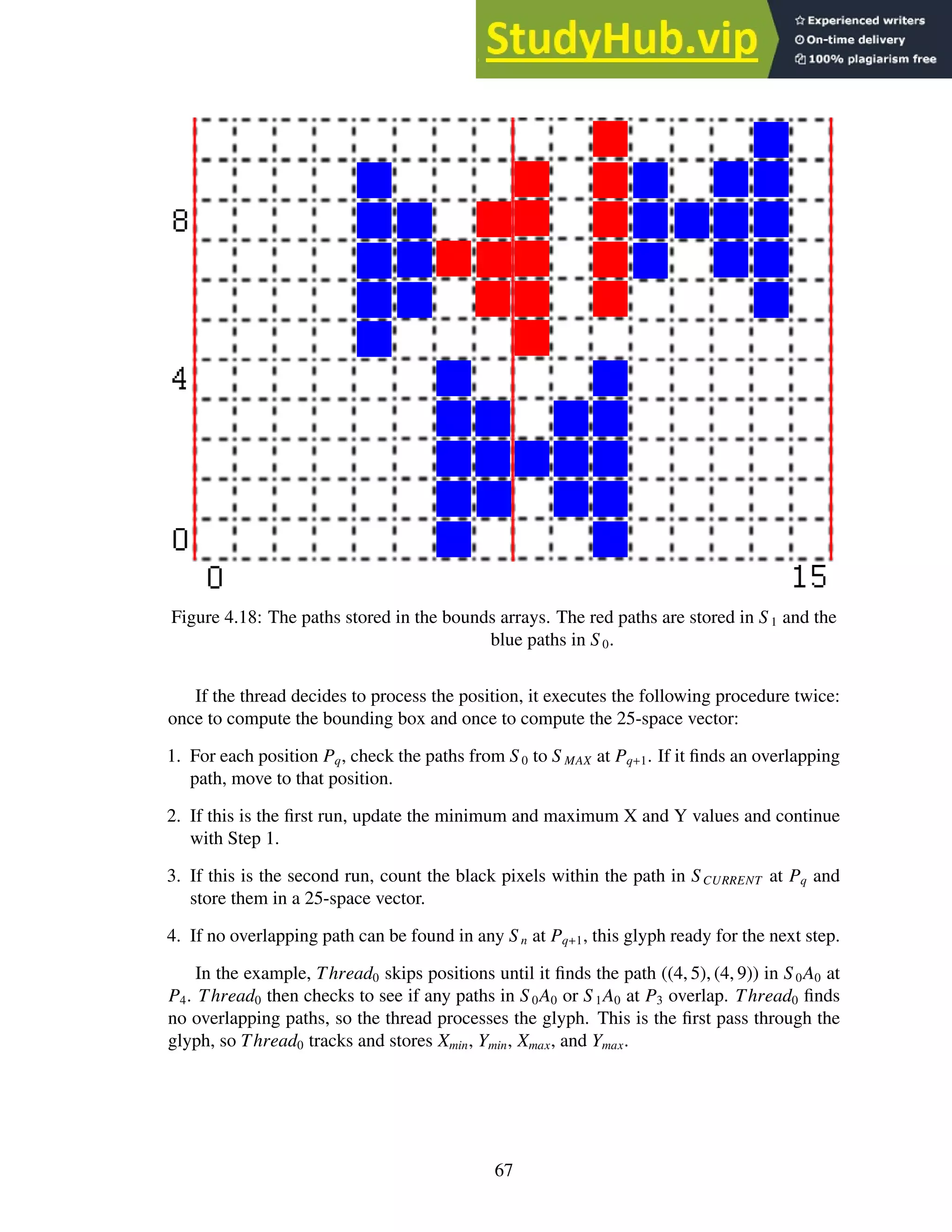
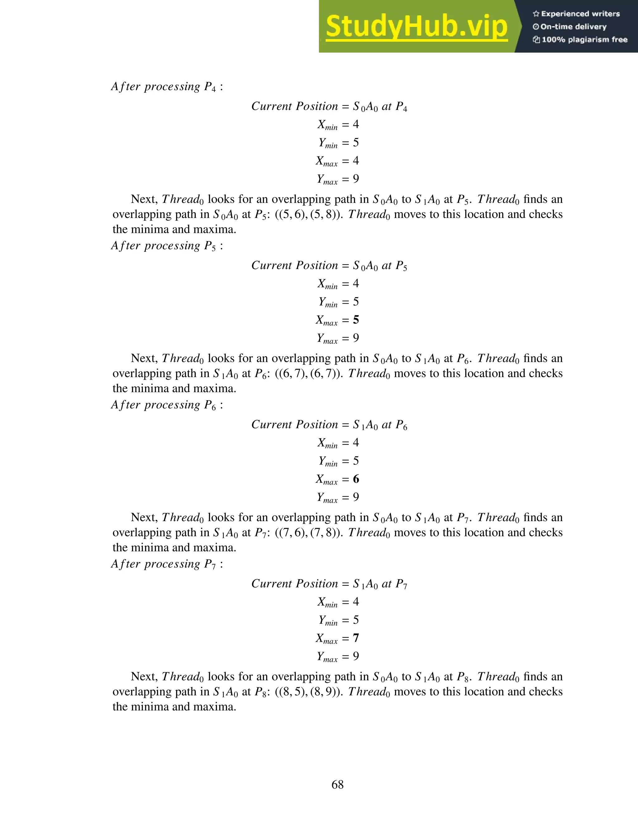
![A fter processing P8 :
Current Position = S 1A0 at P8
Xmin = 4
Ymin = 5
Xmax = 8
Ymax = 9
Next, Thread0 looks for an overlapping path in S0A0 to S 1A0 at P9. Thread0 is unable
to find an overlapping path, so this pass is complete. Thread0 goes back to the starting
position, S 0A0 at P4 and iterates through the glyph again in the same manner. During the
second pass, Thread0 counts the black pixels in the paths at each position it processes and
computes a 25-space vector. The vector computed for the first glyph Thread0 finds is:
(1, 0, 0, 0, 1, 0, 1, 0, 1, 0, 0, 0, 1, 0, 0, 0, 1, 0, 1, 0, 1, 0, 0, 0, 1)
As Thread0 counts pixels, it unsets the processed paths. When Thread0 has finished
processing the first glyph, the bounds arrays look as follows (not taking into account
changes by Thread1):
A fter Thread0 processes the first glyph :
Top1 : [X,X,X,X,X,X,X,X] [X,X,10,X,X,X, X,X]
Bottom1 : [X,X,X,X,X,X,X,X] [X,X, 6,X,X,X, X,X]
Top0 : [X,X,X,X,X,X,4,3] [2,3, 4,9,8,9,10,X]
Bottom0 : [X,X,X,X,X,X,0,1] [2,1, 0,7,8,7, 6,X]
Thread0 is not finished processing S0A0, so it resumes from where it left off and finds
another path in S 0A0 at P6, which indicates a new glyph. Thread0 follows the same proce-
dure to process the new glyph.
Thread1 is operating concurrently with Thread0. The following outlines the actions
Thread1 takes while Thread0 is processing:
1. Thread1 finds the path ((8, 2), (8, 2)) in S 0A1 at P0. Thread1 then checks to see
if any paths in S0A1 or S1A1 at P−1 overlap. Thread1 finds an overlapping path
((7, 1, ), (7, 3)) in S 0A1 at P−1, so Thread1 skips P0.
2. Thread1 finds that S 1A1 at P0 is empty, so the position is skipped.
3. Thread1 finds the path ((9, 1), (9, 3)) in S 0A1 at P1. Thread1 then checks to see
if any paths in S 0A1 or S 1A1 at P0 overlap. Thread1 finds an overlapping path
((8, 2, ), (8, 2)) in S0A1 at P0, so Thread1 skips P1.
4. Thread1 finds that S 1A1 at P1 is empty, so the position is skipped.
5. Thread1 finds the path ((10, 0), (10, 4)) in S 0A1 at P2. Thread1 then checks to see
if any paths in S 0A1 or S 1A1 at P1 overlap. Thread1 finds an overlapping path
((9, 1, ), (9, 3)) in S 0A1 at P1, so Thread1 skips P2.
69](https://image.slidesharecdn.com/anopticalcharacterrecognitionengineforgraphicalprocessingunits-230805215723-24ac1bd2/75/An-Optical-Character-Recognition-Engine-For-Graphical-Processing-Units-82-2048.jpg)
![6. Thread1 finds the path ((10, 6), (10, 10)) in S1A1 at P2. Thread1 then checks to see
if any paths in S 0A1 or S 1A1 at P1 overlap. Thread1 finds no overlapping paths,
so Thread1 processes the glyph using the same procedure already described. The
bounds arrays look as follows (not taking into account changes by Thread0):
A fter Thread1 processes the glyph :
Top1 : [X,X,X,X,X,X,X,X] [X,X,X,X,X,X,X,X]
Bottom1 : [X,X,X,X,X,X,X,X] [X,X,X,X,X,X,X,X]
Top0 : [X,X,X,X,X,X,4,3] [2,3,4,X,X,X,X,X]
Bottom0 : [X,X,X,X,X,X,0,1] [2,1,0,X,X,X,X,X]
7. Thread1 continues processing at the next position. Thread1 finds that S 0A1 at P3 is
empty, so the position is skipped.
8. Thread1 finds that S 1A1 at P3 is empty, so the position is skipped.
9. Thread1 finds that S 0A1 at P4 is empty, so the position is skipped.
10. Thread1 finds that S 1A1 at P4 is empty, so the position is skipped.
11. Thread1 finds that S 0A1 at P5 is empty, so the position is skipped.
12. Thread1 finds that S 1A1 at P5 is empty, so the position is skipped.
13. Thread1 finds that S 0A1 at P6 is empty, so the position is skipped.
14. Thread1 finds that S 1A1 at P6 is empty, so the position is skipped.
15. Thread1 finds that S 0A1 at P7 is empty, so the position is skipped.
16. Thread1 finds that S 1A1 at P7 is empty, so the position is skipped.
17. At this point, Thread1 has completed processing.
The output of this step of the construction stage is a list of best-fit bounding box co-
ordinates and 25-space vectors. Each bounding box and 25-space vector corresponds to a
glyph that was calculated from the bounding polygon of a glyph in the bounds arrays.
The final step of the construction stage is a search of the training data to classify each
glyph. This step searches in the same manner as Version 1 and Version 2.
4.4 Output
The output of the construction stage, stored in global memory, is a list of best-fit bounding
box coordinates, 25-space vectors, and the character classification. The output is down-
loaded from the GPU into host memory and converted to XML. See Figure 4.19 on page
71 for sample XML output.
70](https://image.slidesharecdn.com/anopticalcharacterrecognitionengineforgraphicalprocessingunits-230805215723-24ac1bd2/75/An-Optical-Character-Recognition-Engine-For-Graphical-Processing-Units-83-2048.jpg)
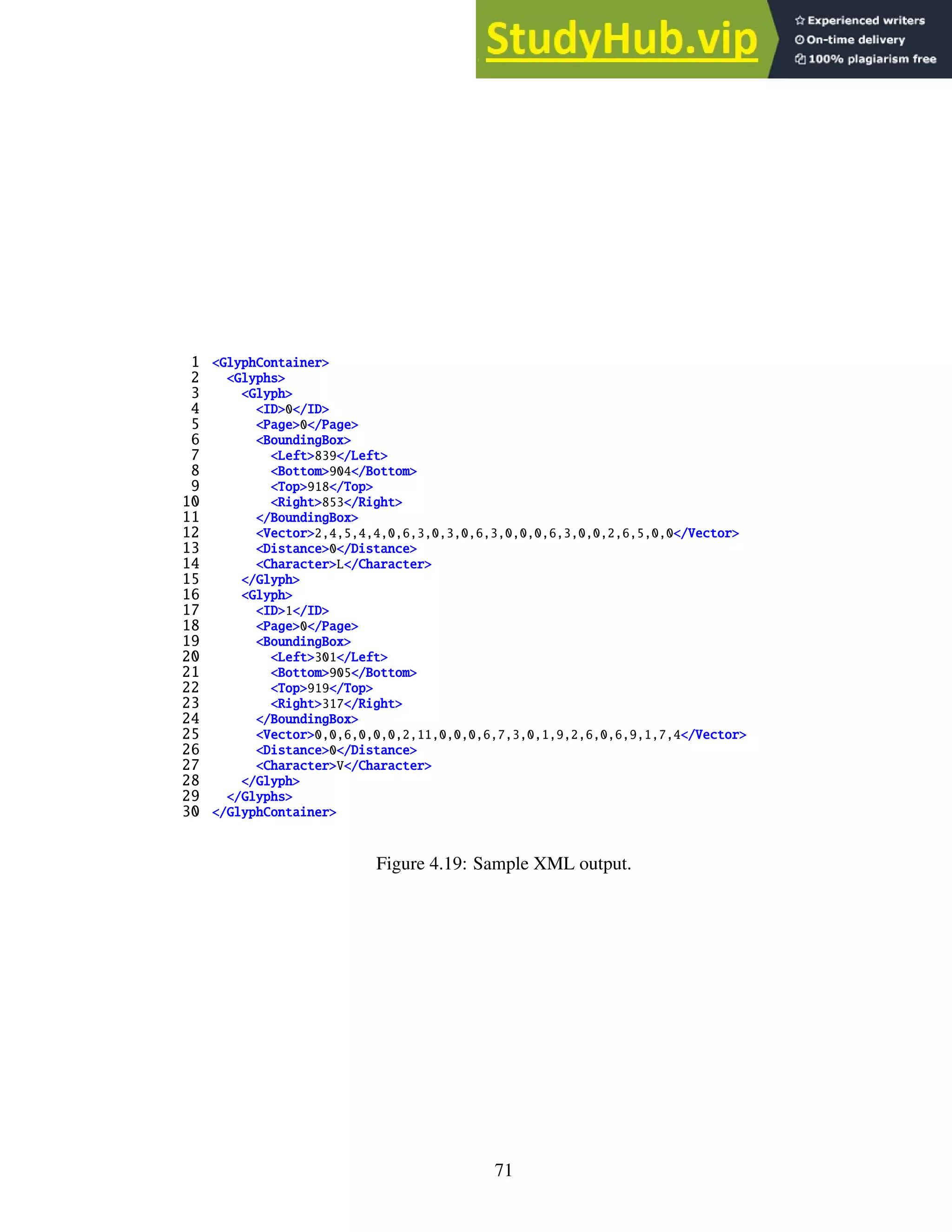
![Chapter 5: Findings and Results
5.1 OCR engines
I test SegRec v3 against Tesseract v3.04.01, ABBYY FineReader Professional 12 and Om-
niPage Ultimate 19. Brief descriptions of each engine can be found below.
Tesseract
Tesseract is an open-source, command-line driven OCR engine that was developed by
Hewlett-Packard and presented at the 1995 UNLV Annual Test of OCR Accuracy [53].
Entered as “HP Labs OCR”, Tesseract consistently scored in the top three (out of eight) for
character recognition accuracy [44]. The version I test against is Tesseract v3.04.011
.
ABBYY FineReader
ABBYY FineReader is a commercial OCR engine by ABBYY. ABBYY was founded in
1989 and ABBYY FineReader debuted in 1993 [2]. According to ABBYY, the ABBYY
FineReader software is used by over 30 million people world-wide. The version I test
against is ABBYY FineReader 12 Professional2
.
OmniPage Ultimate
OmniPage Ultimate is a commercial OCR engine by Nuance. Nuance’s products are in use
by over 22 million users [33]. The version I test against is OmniPage Ultimate 193
.
5.2 Image set creation
Normal set
I programatically generated one thousand 8.5”×11” page images of “lorem ipsum”4
using a
12pt “Courier New” font. These page images are flawless and should be easily recognizable
by all engines. This set of page images is the “normal” set. See Figure B.1 in Appendix B
on page 86 for a sample page.
1
Tesseract can be downloaded from https://github.com/tesseract-ocr
2
A trial version of ABBYY FineReader can be downloaded from https://www.abbyy.com/en-us/
finereader/professional/
3
A trial version of OmniPage Ultimate can be downloaded from http://www.nuance.com/
for-business/by-product/omnipage/ultimate/index.htm.
4
Lorem Ipsum is the printing and typesetting industry standard dummy text. See http://www.lipsum.
com/ for more information.
72](https://image.slidesharecdn.com/anopticalcharacterrecognitionengineforgraphicalprocessingunits-230805215723-24ac1bd2/75/An-Optical-Character-Recognition-Engine-For-Graphical-Processing-Units-85-2048.jpg)
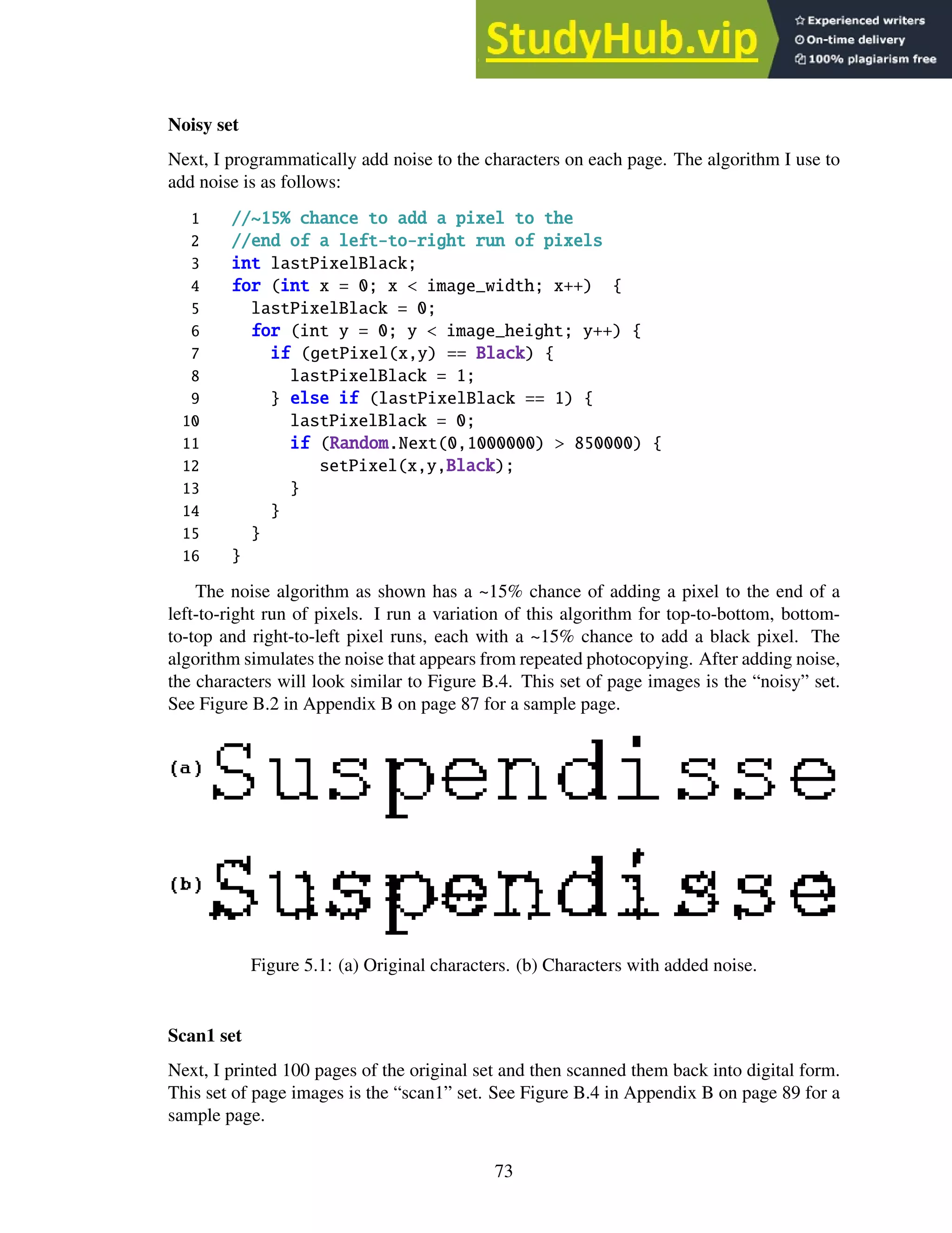
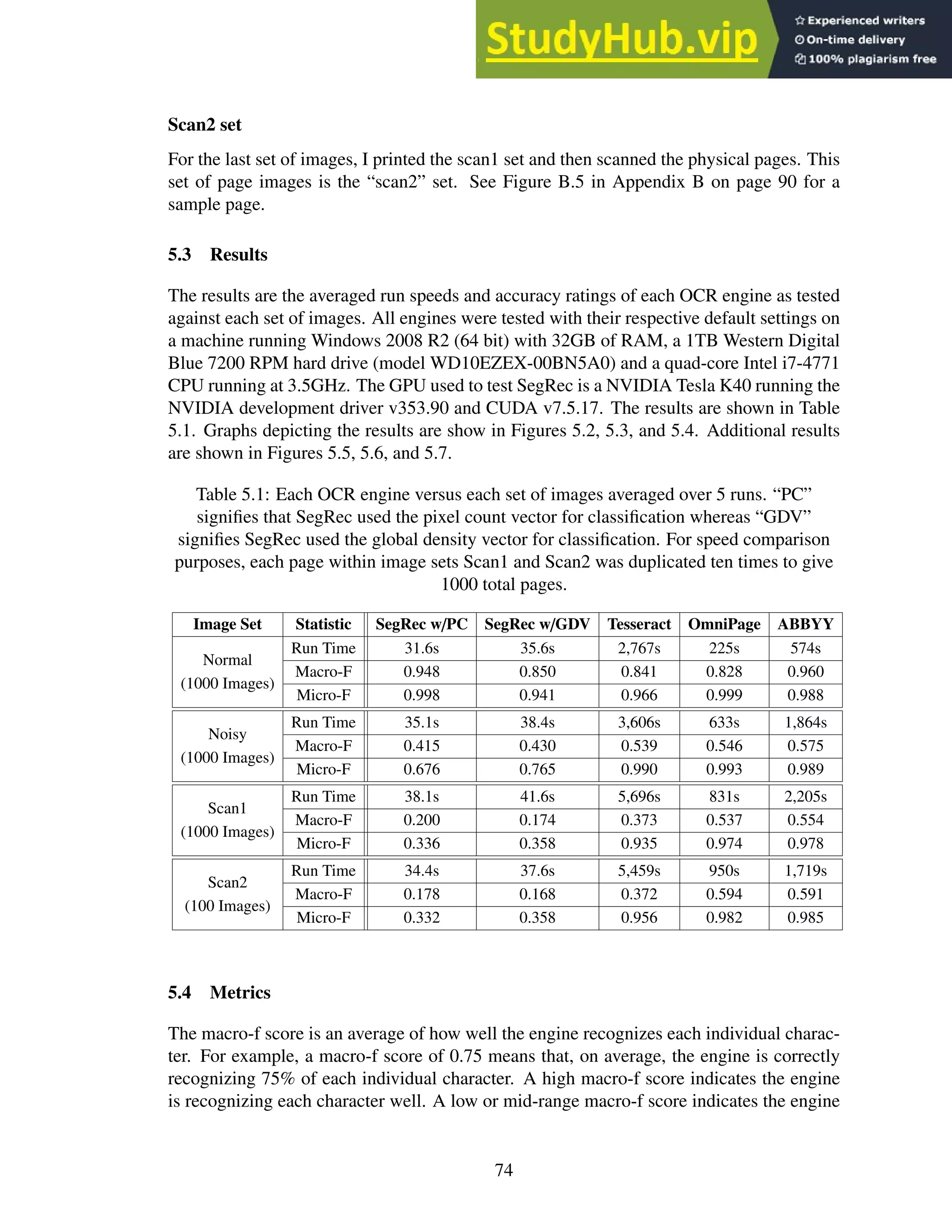
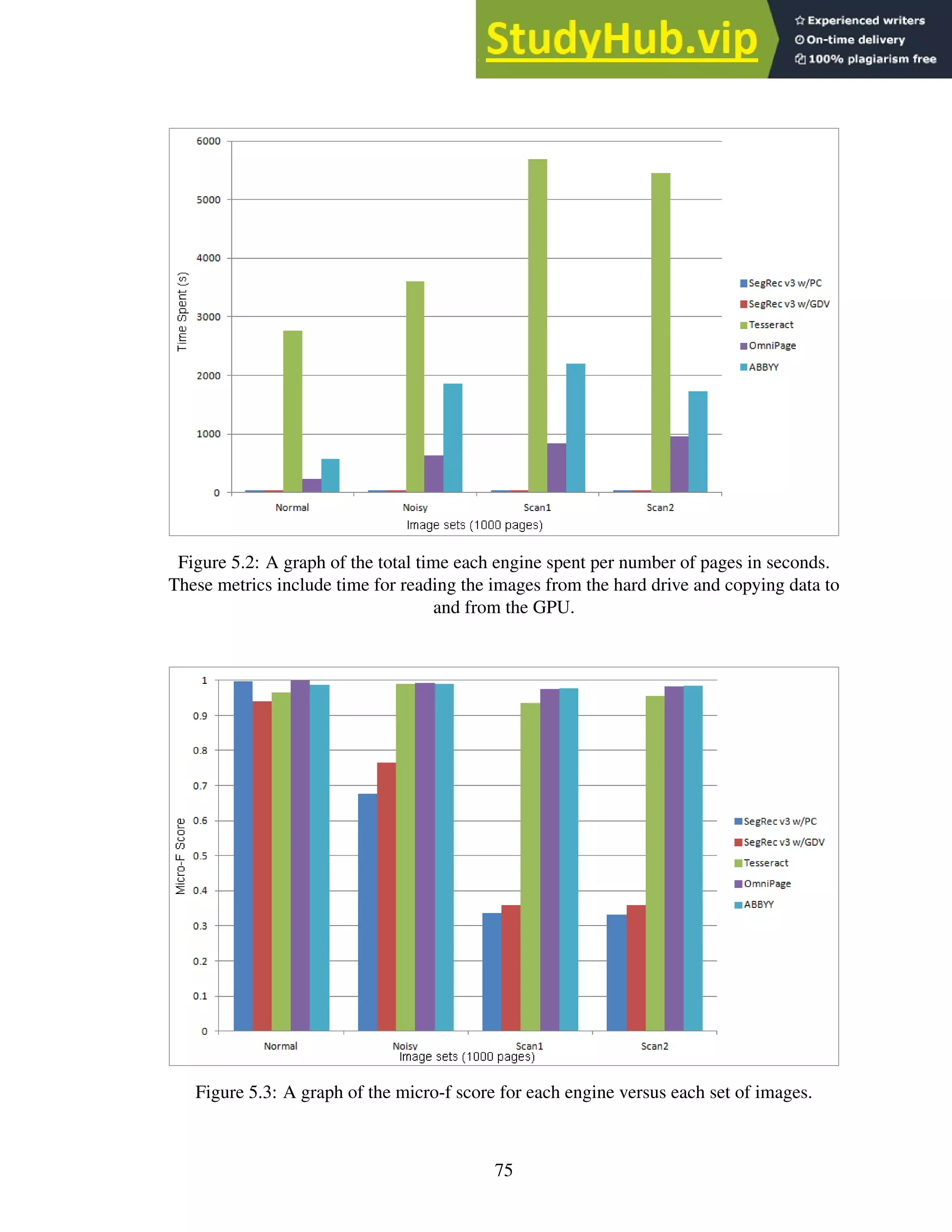
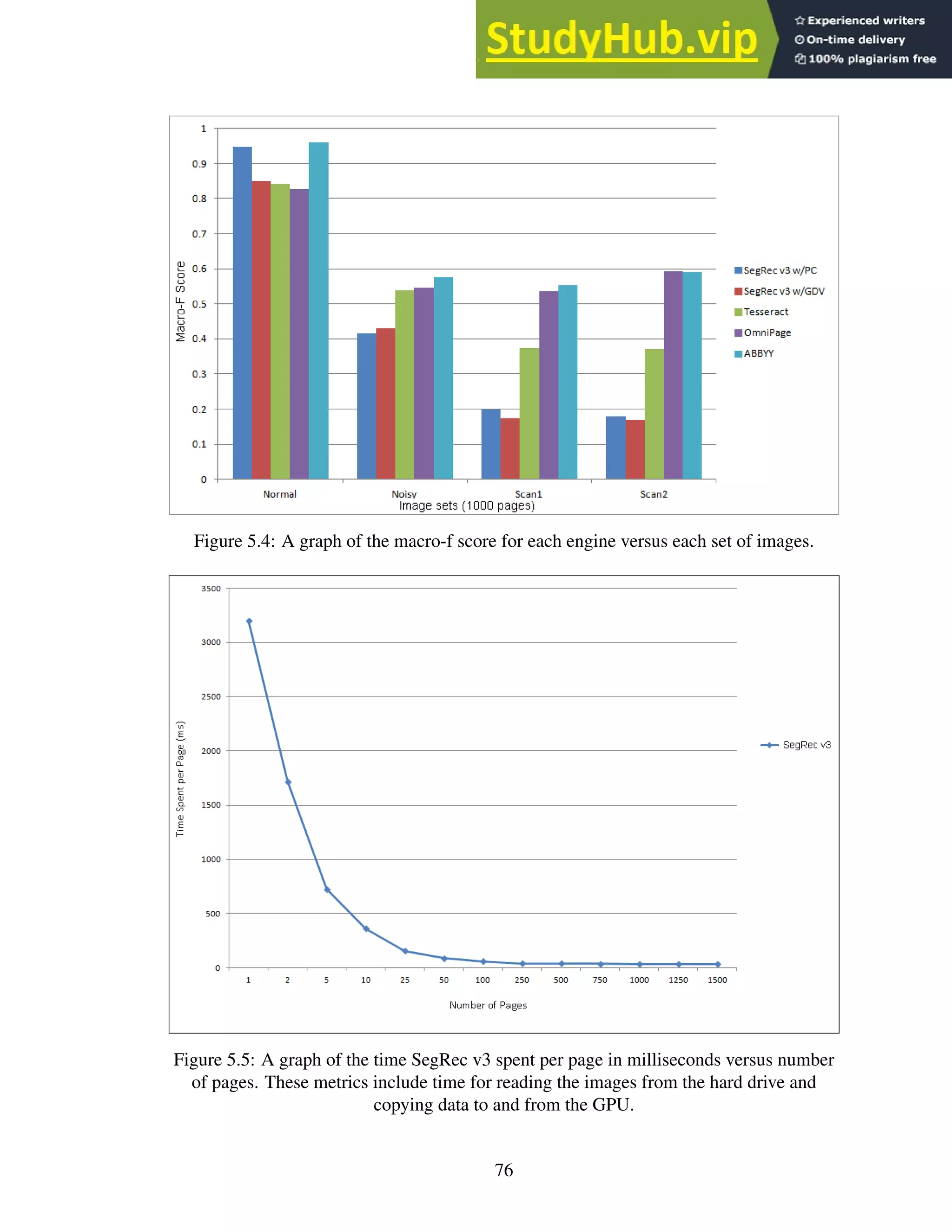
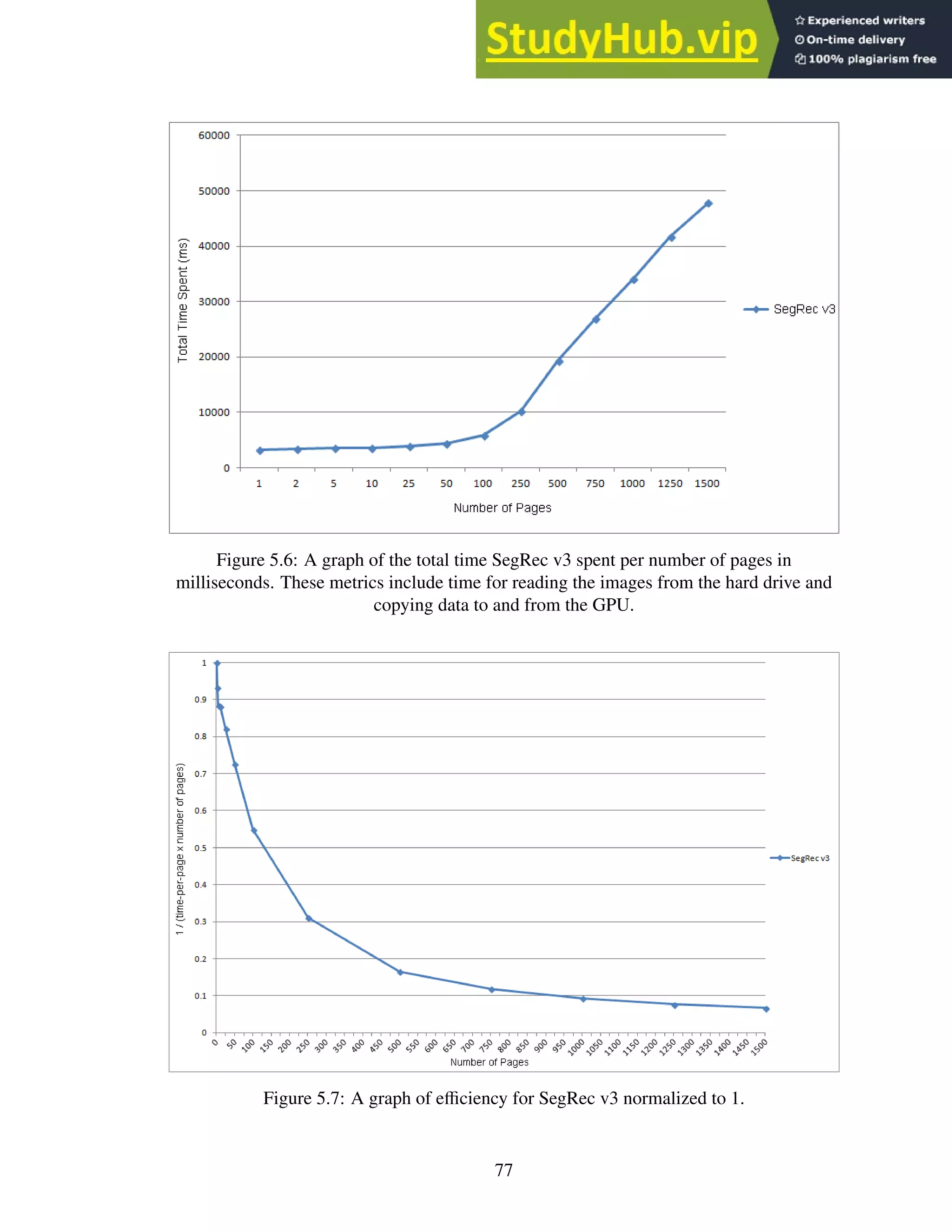
![is recognizing at least some of the characters poorly. The micro-f score is the weighted av-
erage of how well the engine recognizes each character, with the weight of each character
reflecting how many times the character appears in the text. For example, a micro-f score
of 0.75 means that the engine is correctly recognizing 75% of the total character count,
regardless of the type of character. A high micro-f score indicates that the engine is rec-
ognizing the vast majority of characters correctly and vice versa for a low or mid-range
micro-f score. See Appendix A for a more in-depth discussion on the macro-f and micro-f
metrics.
5.5 Discussion: Software limitations
I chose to implement SegRec v3 in C#.NET, which interfaces with CUDA via a third-party
library called Cudafy.NET. Unfortunately, .NET has a ~2GB file limit size, which limits
the amount of data I can read and push to the GPU in a single interaction. This limit is
reached at approximately 1500 pages of text, which is why SegRec v3 test results only
include results up to 1500 pages. The Tesla K40 GPU I test on is capable of supporting
up to 12GB of data, which should hold approximately 9000 pages of text, given SegRec
v3’s current memory requirements. I plan to rewrite the .NET portion of SegRec v3 in a
language that does not have such file size limitations in the future.
5.6 Discussion: Speed
Figure 5.5 shows the speed per page for SegRec v3 when running various numbers of
pages. Figure 5.6 shows the total time taken by SegRec v3 when running various num-
bers of pages. The data shows that as SegRec v3 processes more pages, the time spent
per page decreases in a non-linear fashion. In my experience, this decrease is typical of
GPU processing. The reason for that is because the GPU tries to hide the latency of I/O
operations. The GPU has been optimized so that context switching between threads costs
almost nothing. So, when a thread warp issues an I/O operation and is idle while waiting
for the instruction to complete, such as a global memory read or write (SegRec v3 uses
global memory to store image and output data), the GPU will switch to a thread warp that
is ready to execute instructions. In other words, the GPU pipelines I/O and takes advantage
of nearly free context switches to minimize time spent actively executing idle warps and to
maximize instruction execution throughput [34].
5.7 Discussion: Image sets
Normal image set
SegRec is significantly faster than any other engine, with a speedup of ×88 over Tesseract,
×7 over OmniPage Ultimate, and ×18 over ABBYY FineReader. All engines have high
micro-f measures, meaning each engine recognizes the majority of characters correctly.
The relatively low macro-f scores for SegRec w/GDC, Tesseract and Omnipage combined
with the high micro-f scores indicate these engines struggle to recognize several character
types. Examining the full character result tables in D, we see that SegRec w/GDC struggles
78](https://image.slidesharecdn.com/anopticalcharacterrecognitionengineforgraphicalprocessingunits-230805215723-24ac1bd2/75/An-Optical-Character-Recognition-Engine-For-Graphical-Processing-Units-91-2048.jpg)
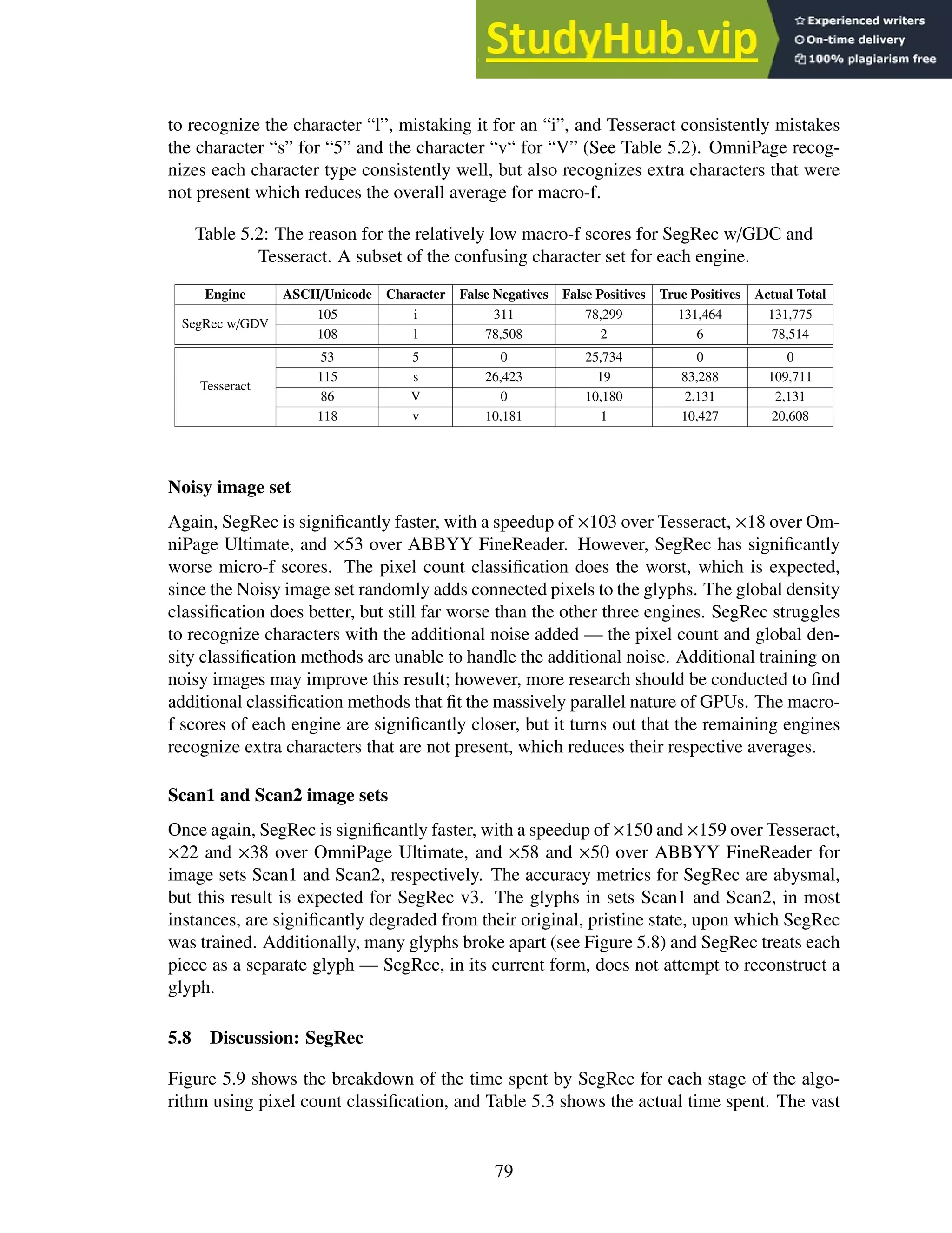
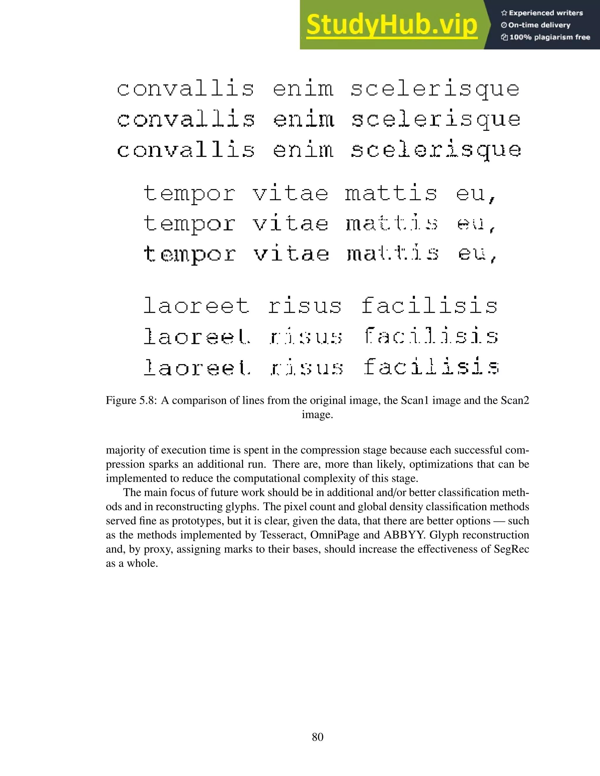
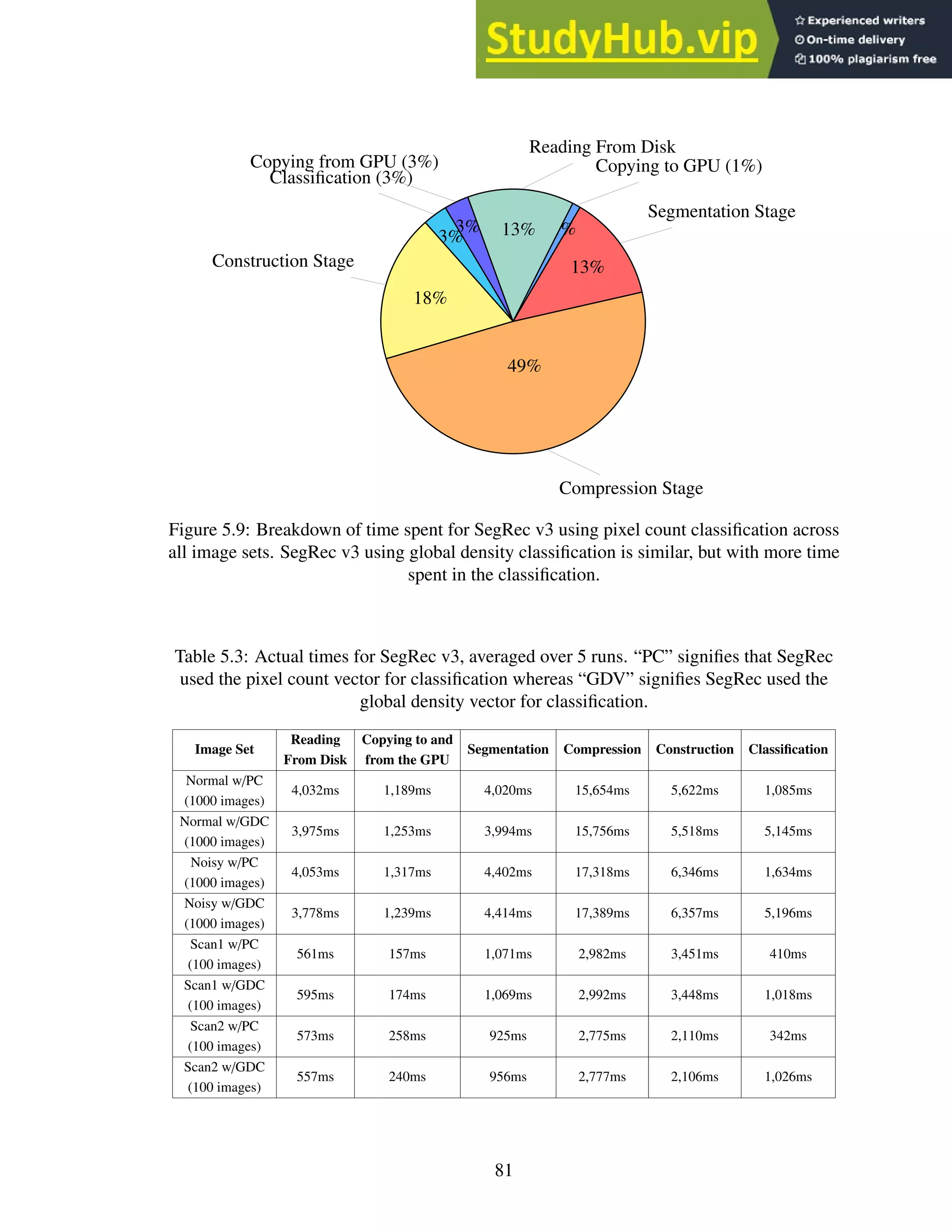
![Appendix A: Measures of accuracy and precision for OCR
Figure A.1: Table for binary classification.
Adapted from http://en.wikipedia.org/wiki/Accuracy_and_precision
For a binary decision, the definitions of accuracy and precision are defined as follows:
• Accuracy:
true positives + true negatives
true positives + true negatives + false positives + false negatives
• Precision:
true positives
true positives + false positives
Additional useful statistical measures:
• Recall:
true positives
true positives + false negatives
• F-measure:
2 ·
Precision · Recall
Precision + Recall
For OCR, the notion of “true negative” is removed because it no longer applies — the
OCR engine can only reply with an answer from the alphabet, it cannot respond “not-A”,
for example. The key concept for multinary classification, as relevant to OCR engines, is
that an incorrect answer by the OCR engine counts as both a “false positive” and a “false
negative“. The answer counts as a false positive for the incorrect character presented as
the answer and as a false negative for the answer that should have been presented. For
example, if the answer is “A” and the engine responds with a “B”, the response counts as
a false positive for B and a false negative for A. A full classification table for the alphabet
[A, B,C] is shown in Figure A.2.
The statistical measures for multinary classification are called micro and macro av-
eraging of F-measures. Macro averaging incorporates the base formulae for precision,
recall and F-measure to calculate a value for an entire system. For a given alphabet, A, the
equation for macro averaging is as follows:
84](https://image.slidesharecdn.com/anopticalcharacterrecognitionengineforgraphicalprocessingunits-230805215723-24ac1bd2/75/An-Optical-Character-Recognition-Engine-For-Graphical-Processing-Units-97-2048.jpg)
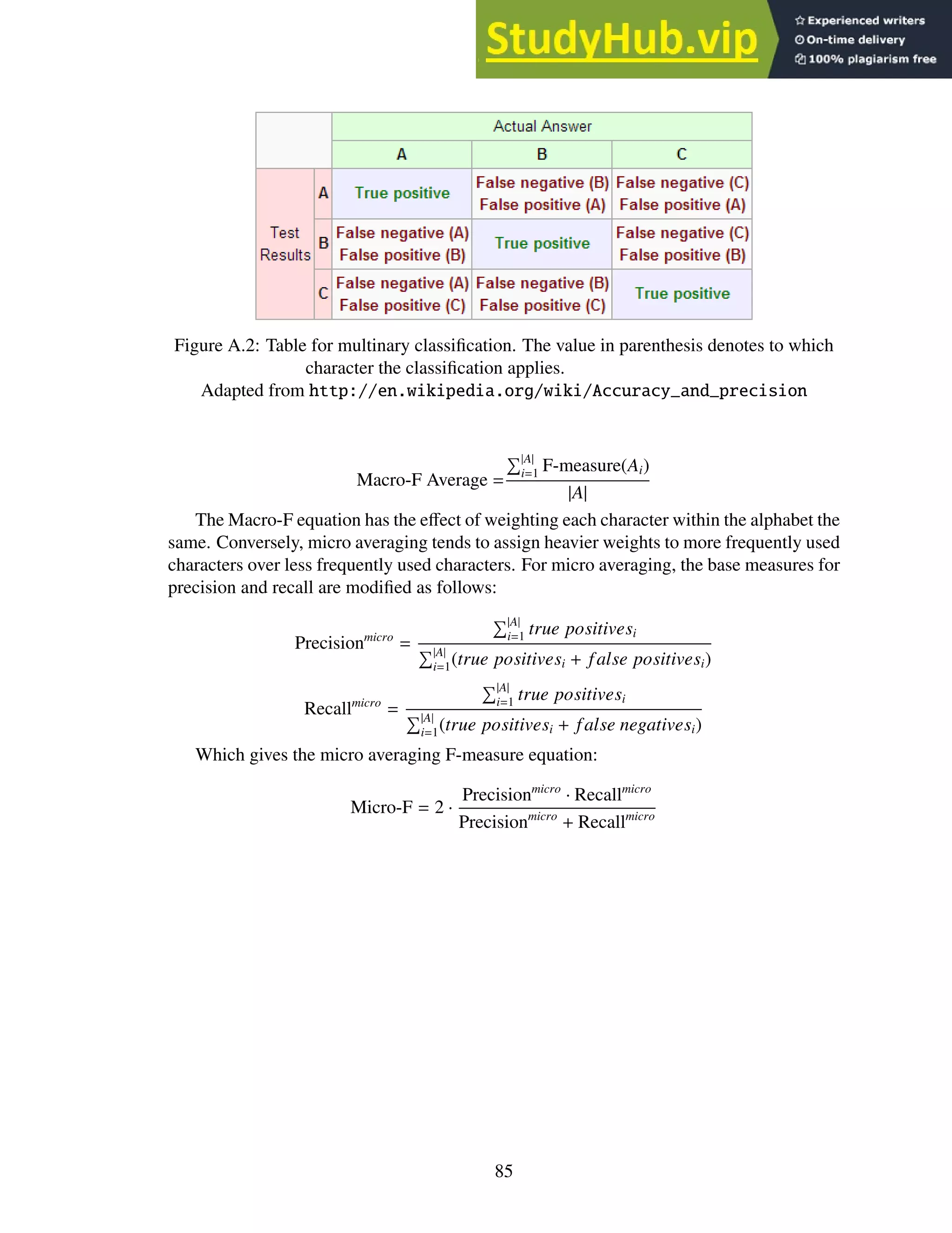
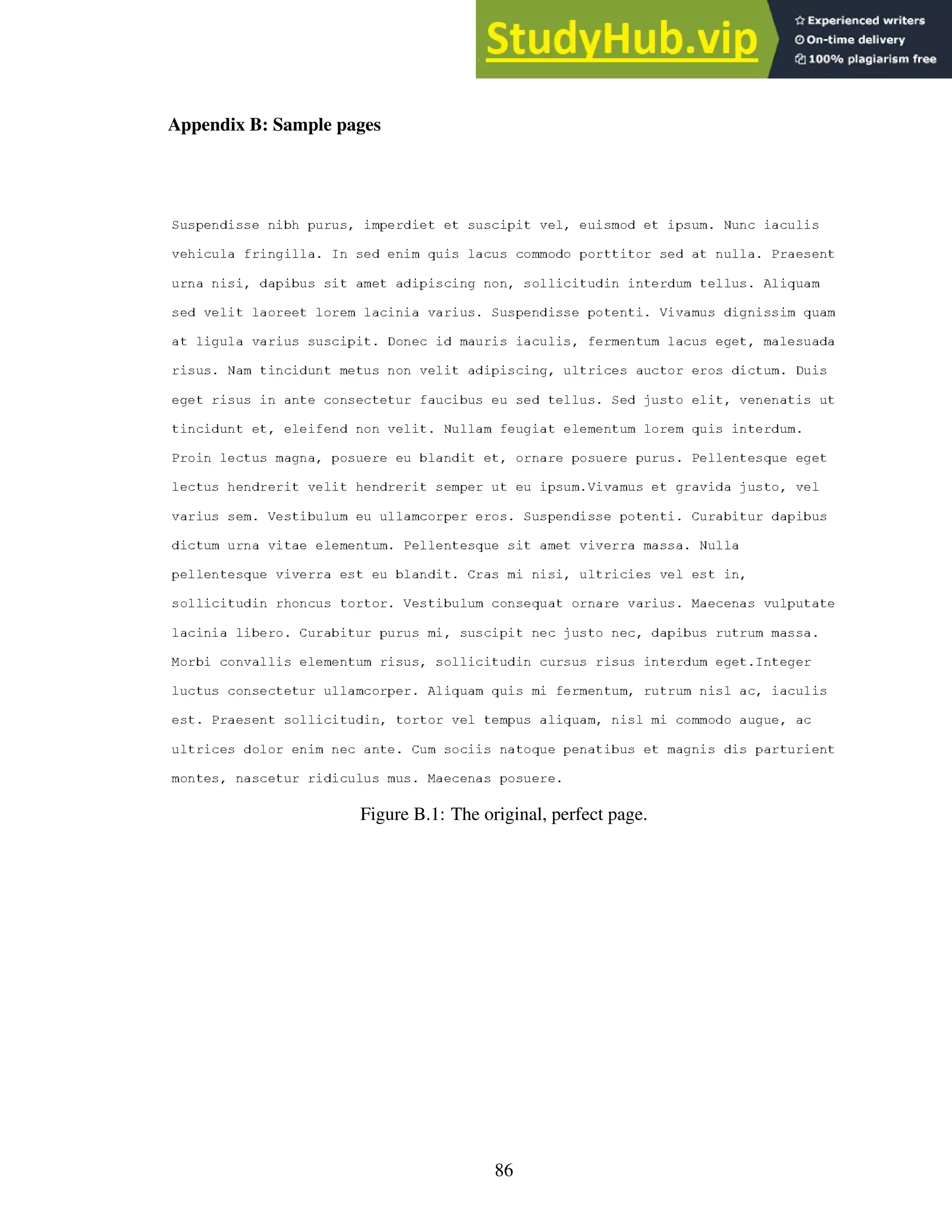

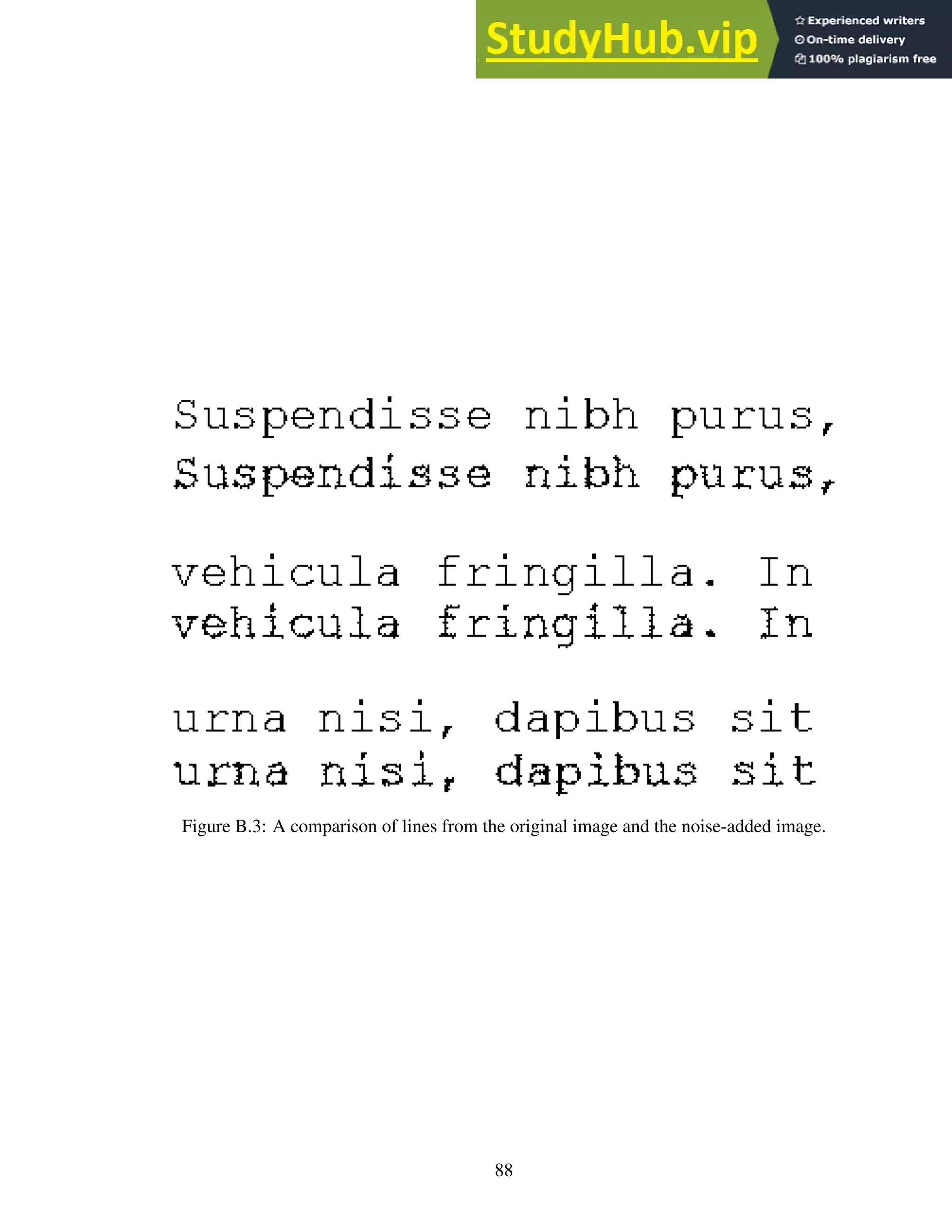
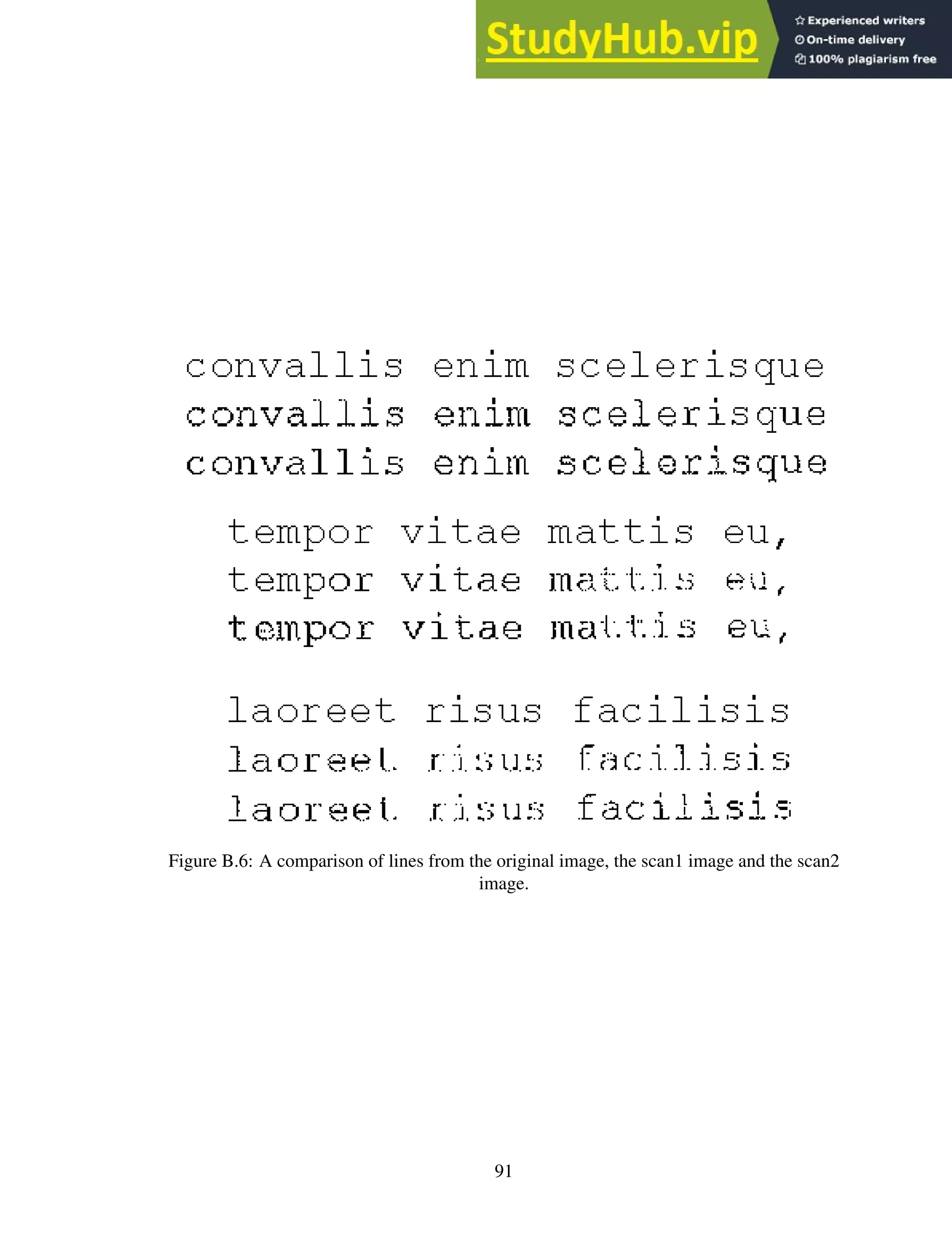
![Appendix C: Avoiding branching with inline Boolean expressions
This section addresses the question of whether inline Boolean expressions avoid branching
on NVIDIA hardware. In CUDA C, inline Boolean expressions evaluate to 1 for true and
0 for false. A shrewd programmer can take advantage of this fact.
The two functions, example1 and example2, written in CUDA C and shown in Figures
C.1 and C.2, respectively, are functionally identical. Function example1 contains several
nested if statements, and function example2 implements the same functionality with inline
Boolean statements. The compiled PTX1
code for example1 is in Figure C.3 and C.4. The
branching instructions in the figures are highlighted in red, and the labels, which serve as
jump targets, are highlighted in purple. Figure C.5 contains the code for example2. It
contains no branch instructions or jump targets. Clearly, using inline Boolean expressions
avoids branching.
However, threads running example2 might execute many more instructions overall,
so whether avoiding branching actually helps increase execution speed remains unclear.
Benchmarking and testing can determine which function will perform the best given real-
world data. The tests and results that follow were conducted and gathered using a GTX
480.
A grid of 65,535 blocks each containing 1,024 threads executes each function — a total
of 67,107,840 executions per function — and Table C.1 provides the results given by the
NVIDIA command-line profiler, nvprov2
. Branch efficiency, the ratio of non-divergent
branches to total branches, is controlled by altering the input data to force example1 to
execute a specific code path out of the four alternatives3
. Table C.1 compares the execu-
tion time of example1 and example2 at several different branch efficiencies. As branch
efficiency decreases, the run-time of example1 increases, while the run-time of example2
remains relatively constant. This is the predicted behavior. Unexpectedly, the run-time for
example1 at 100% branch efficiency is about 1ms slower than example2.
Table C.2 is a subset of the metrics available from nvprof (full list shown in Table C.3)
and contains metrics where the values gathered by nvprof for each function differ by a sig-
nificant amount. The first metric shown, “Executed Instructs Per Cycle”, provides a reason
for the difference in speed. Even at 100% branch efficiency, the function example1 had
a much lower executed instruction throughput than example2. I hypothesize that the rea-
son for the difference in throughput is the additional number of control-flow instructions4
executed by example1. The data in Table C.2 seems to support this hypothesis. Over the
course of the ~67M function executions, example1 issues and executes 4× more control-
flow instructions than example25
(8,388,840 to 2,097,120). This metric is the only instruc-
1
PTX is an assembly-like language generated by the NVIDIA CUDA compiler and is used by NVIDIA’s
GPUs [34, 35].
2
NVIDIA’s command-line profiler, nvprov, provides information such as run-time, occupancy, and
throughput among a myriad of other metrics [36].
3
The code paths are labeled via comments — see Figure C.1.
4
Control-flow instructions are PTX instructions related to if, switch, do, for, and while statements [34].
5
Remember that NVIDIA GPUs operate with the SIMT (Single Instruction, Multiple Threads) architec-
92](https://image.slidesharecdn.com/anopticalcharacterrecognitionengineforgraphicalprocessingunits-230805215723-24ac1bd2/75/An-Optical-Character-Recognition-Engine-For-Graphical-Processing-Units-105-2048.jpg)
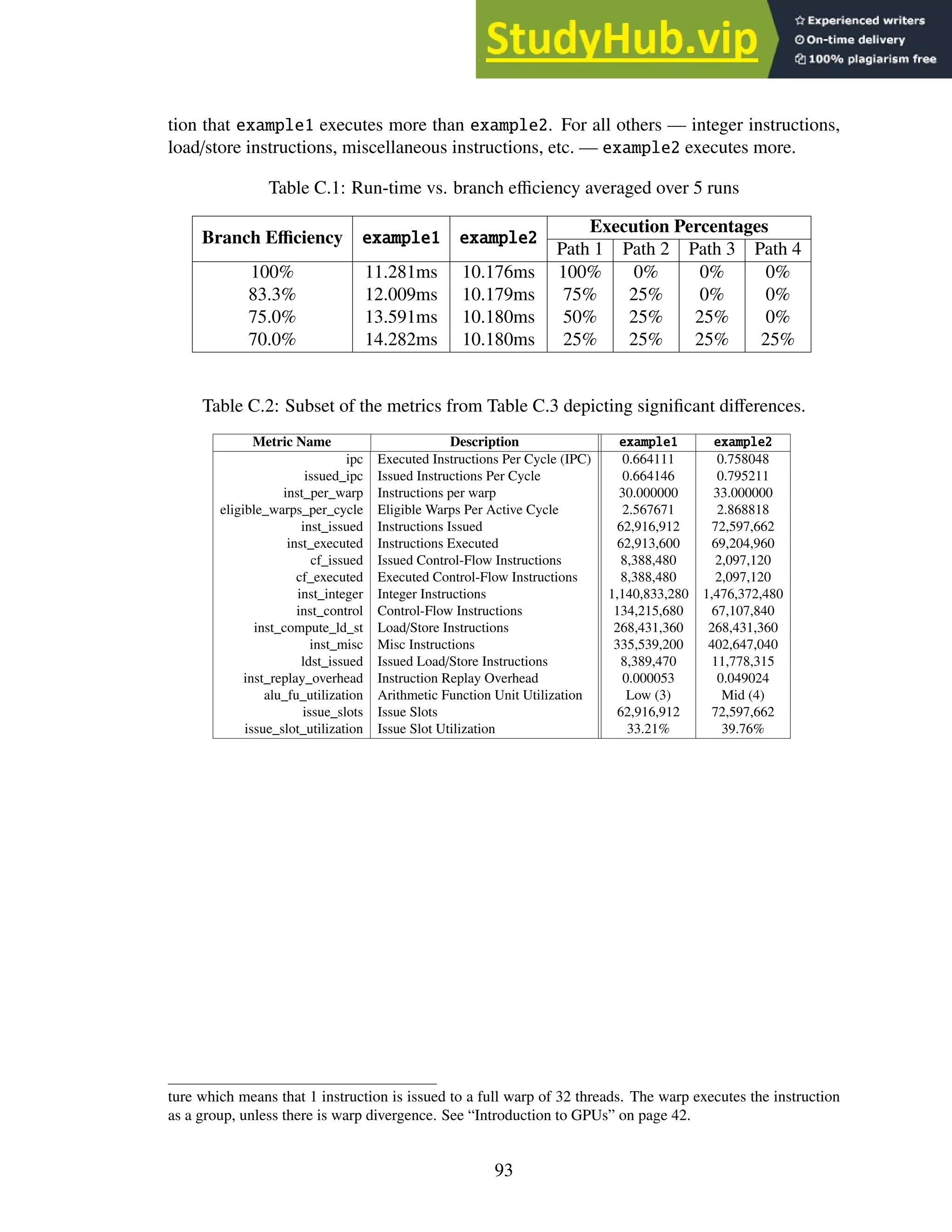
![1 __global__ void check1(int* a, int* b, int* c, int* d) {
2 // calculate global thread ID
3 int gID = blockIdx.x * blockDim.x + threadIdx.x;
4 if (a[gID] < b[gID]) {
5 if (((b[gID] - a[gID]) * 2 + 1) <= (c[gID] % 5))
6 d[gID] = 1; // path 1
7 else
8 d[gID] = 0; // path 2
9 } else if (a[gID] >= b[gID]) {
10 if (((a[gID] - b[gID]) * 2) <= (c[gID] % 5))
11 d[gID] = 1; // path 3
12 else
13 d[gID] = 0; // path 4
14 }
15 }
Figure C.1: CUDA C version of function example1.
1 __global__ void check2(int* a, int* b, int* c, int* d) {
2 // calculate global thread ID
3 int gID = blockIdx.x * blockDim.x + threadIdx.x;
4 d[gID] = (a[gID] < b[gID]) * (((b[gID] - a[gID]) * 2 + 1) <= (c[gID] % 5))
5 + (a[gID] >= b[gID]) * (((a[gID] - b[gID]) * 2) <= (c[gID] % 5));
6 }
Figure C.2: CUDA C version of function example2.
94](https://image.slidesharecdn.com/anopticalcharacterrecognitionengineforgraphicalprocessingunits-230805215723-24ac1bd2/75/An-Optical-Character-Recognition-Engine-For-Graphical-Processing-Units-107-2048.jpg)
![1 .version 4.2
2 .target sm_20
3 .address_size 64
4
5 .visible .entry _example1(
6 .param .u64 _example1_param_0,
7 .param .u64 _example1_param_1,
8 .param .u64 _example1_param_2,
9 .param .u64 _example1_param_3
10 )
11 {
12 .reg .pred %p<5>;
13 .reg .s32 %r<29>;
14 .reg .s64 %rd<14>;
15
16 ld.param.u64 %rd3, [_example1_param_0];
17 ld.param.u64 %rd4, [_example1_param_1];
18 ld.param.u64 %rd5, [_example1_param_2];
19 ld.param.u64 %rd6, [_example1_param_3];
20 cvta.to.global.u64 %rd7, %rd6;
21 mov.u32 %r3, %ntid.x;
22 mov.u32 %r4, %ctaid.x;
23 mov.u32 %r5, %tid.x;
24 mad.lo.s32 %r6, %r3, %r4, %r5;
25 cvta.to.global.u64 %rd8, %rd3;
26 mul.wide.s32 %rd9, %r6, 4;
27 add.s64 %rd10, %rd8, %rd9;
28 cvta.to.global.u64 %rd11, %rd4;
29 add.s64 %rd12, %rd11, %rd9;
30 ld.global.u32 %r1, [%rd12];
31 ld.global.u32 %r2, [%rd10];
32 setp.lt.s32 %p1, %r2, %r1;
33 cvta.to.global.u64 %rd13, %rd5;
34 add.s64 %rd1, %rd13, %rd9;
35 add.s64 %rd2, %rd7, %rd9;
36 @%p1 bra BB0_4;
37 bra.uni BB0_1;
38
39 BB0_4:
40 sub.s32 %r18, %r1, %r2;
41 shl.b32 %r19, %r18, 1;
42 ld.global.u32 %r20, [%rd1];
43 mul.hi.s32 %r21, %r20, 1717986919;
44 shr.u32 %r22, %r21, 31;
45 shr.s32 %r23, %r21, 1;
46 add.s32 %r24, %r23, %r22;
47 mul.lo.s32 %r25, %r24, 5;
48 sub.s32 %r26, %r20, %r25;
49 setp.lt.s32 %p3, %r19, %r26;
50 @%p3 bra BB0_6;
51 bra.uni BB0_5;
52
53 BB0_6:
54 mov.u32 %r28, 1;
55 st.global.u32 [%rd2], %r28;
56 bra.uni BB0_7;
57
58
Figure C.3: PTX version of function example1.
95](https://image.slidesharecdn.com/anopticalcharacterrecognitionengineforgraphicalprocessingunits-230805215723-24ac1bd2/75/An-Optical-Character-Recognition-Engine-For-Graphical-Processing-Units-108-2048.jpg)
![59 BB0_1:
60 sub.s32 %r7, %r2, %r1;
61 shl.b32 %r8, %r7, 1;
62 ld.global.u32 %r9, [%rd1];
63 mul.hi.s32 %r10, %r9, 1717986919;
64 shr.u32 %r11, %r10, 31;
65 shr.s32 %r12, %r10, 1;
66 add.s32 %r13, %r12, %r11;
67 mul.lo.s32 %r14, %r13, 5;
68 sub.s32 %r15, %r9, %r14;
69 setp.gt.s32 %p2, %r8, %r15;
70 @%p2 bra BB0_3;
71 bra.uni BB0_2;
72
73 BB0_3:
74 mov.u32 %r17, 0;
75 st.global.u32 [%rd2], %r17;
76 bra.uni BB0_7;
77
78 BB0_5:
79 mov.u32 %r27, 0;
80 st.global.u32 [%rd2], %r27;
81 bra.uni BB0_7;
82
83 BB0_2:
84 mov.u32 %r16, 1;
85 st.global.u32 [%rd2], %r16;
86
87 BB0_7:
88 ret;
89 }
Figure C.4: PTX version of function example1 continued.
96](https://image.slidesharecdn.com/anopticalcharacterrecognitionengineforgraphicalprocessingunits-230805215723-24ac1bd2/75/An-Optical-Character-Recognition-Engine-For-Graphical-Processing-Units-109-2048.jpg)
![1 .version 4.2
2 .target sm_20
3 .address_size 64
4
5 // .globl _example2
6
7 .visible .entry _example2(
8 .param .u64 _example2_param_0,
9 .param .u64 _example2_param_1,
10 .param .u64 _example2_param_2,
11 .param .u64 _example2_param_3
12 )
13 {
14 .reg .pred %p<7>;
15 .reg .s32 %r<21>;
16 .reg .s64 %rd<14>;
17
18 ld.param.u64 %rd1, [_example2_param_0];
19 ld.param.u64 %rd2, [_example2_param_1];
20 ld.param.u64 %rd3, [_example2_param_2];
21 ld.param.u64 %rd4, [_example2_param_3];
22 cvta.to.global.u64 %rd5, %rd4;
23 cvta.to.global.u64 %rd6, %rd3;
24 cvta.to.global.u64 %rd7, %rd2;
25 cvta.to.global.u64 %rd8, %rd1;
26 mov.u32 %r1, %ctaid.x;
27 mov.u32 %r2, %ntid.x;
28 mov.u32 %r3, %tid.x;
29 mad.lo.s32 %r4, %r2, %r1, %r3;
30 mul.wide.s32 %rd9, %r4, 4;
31 add.s64 %rd10, %rd8, %rd9;
32 ld.global.u32 %r5, [%rd10];
33 add.s64 %rd11, %rd7, %rd9;
34 ld.global.u32 %r6, [%rd11];
35 setp.gt.s32 %p1, %r6, %r5;
36 sub.s32 %r7, %r6, %r5;
37 shl.b32 %r8, %r7, 1;
38 add.s64 %rd12, %rd6, %rd9;
39 ld.global.u32 %r9, [%rd12];
40 mul.hi.s32 %r10, %r9, 1717986919;
41 shr.u32 %r11, %r10, 31;
42 shr.s32 %r12, %r10, 1;
43 add.s32 %r13, %r12, %r11;
44 mul.lo.s32 %r14, %r13, 5;
45 sub.s32 %r15, %r9, %r14;
46 setp.lt.s32 %p2, %r8, %r15;
47 and.pred %p3, %p2, %p1;
48 selp.u32 %r16, 1, 0, %p3;
49 setp.gt.s32 %p4, %r5, %r6;
50 sub.s32 %r17, %r5, %r6;
51 shl.b32 %r18, %r17, 1;
52 setp.le.s32 %p5, %r18, %r15;
53 and.pred %p6, %p5, %p4;
54 selp.u32 %r19, 1, 0, %p6;
55 add.s32 %r20, %r19, %r16;
56 add.s64 %rd13, %rd5, %rd9;
57 st.global.u32 [%rd13], %r20;
58 ret;
59 }
Figure C.5: PTX version of function example2.
97](https://image.slidesharecdn.com/anopticalcharacterrecognitionengineforgraphicalprocessingunits-230805215723-24ac1bd2/75/An-Optical-Character-Recognition-Engine-For-Graphical-Processing-Units-110-2048.jpg)
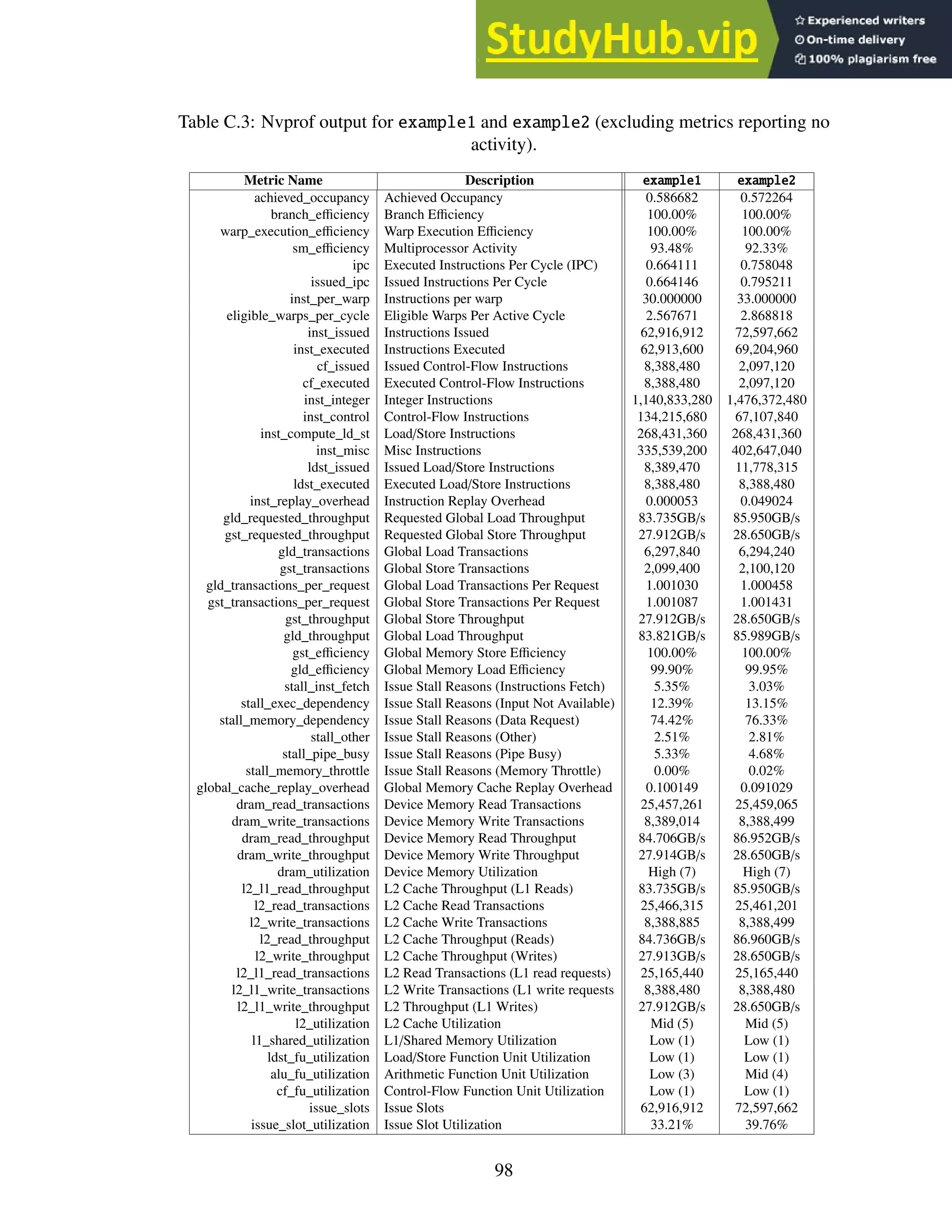


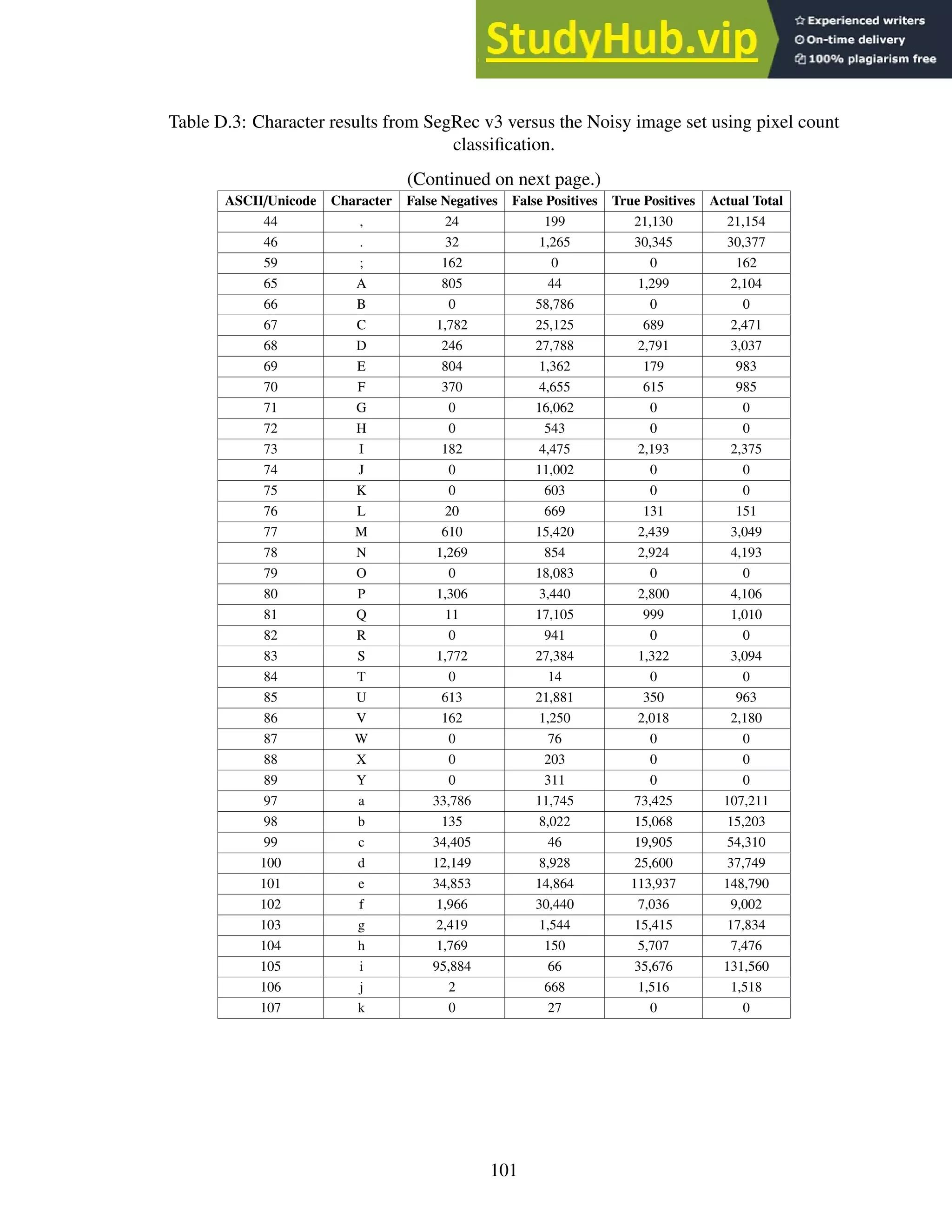


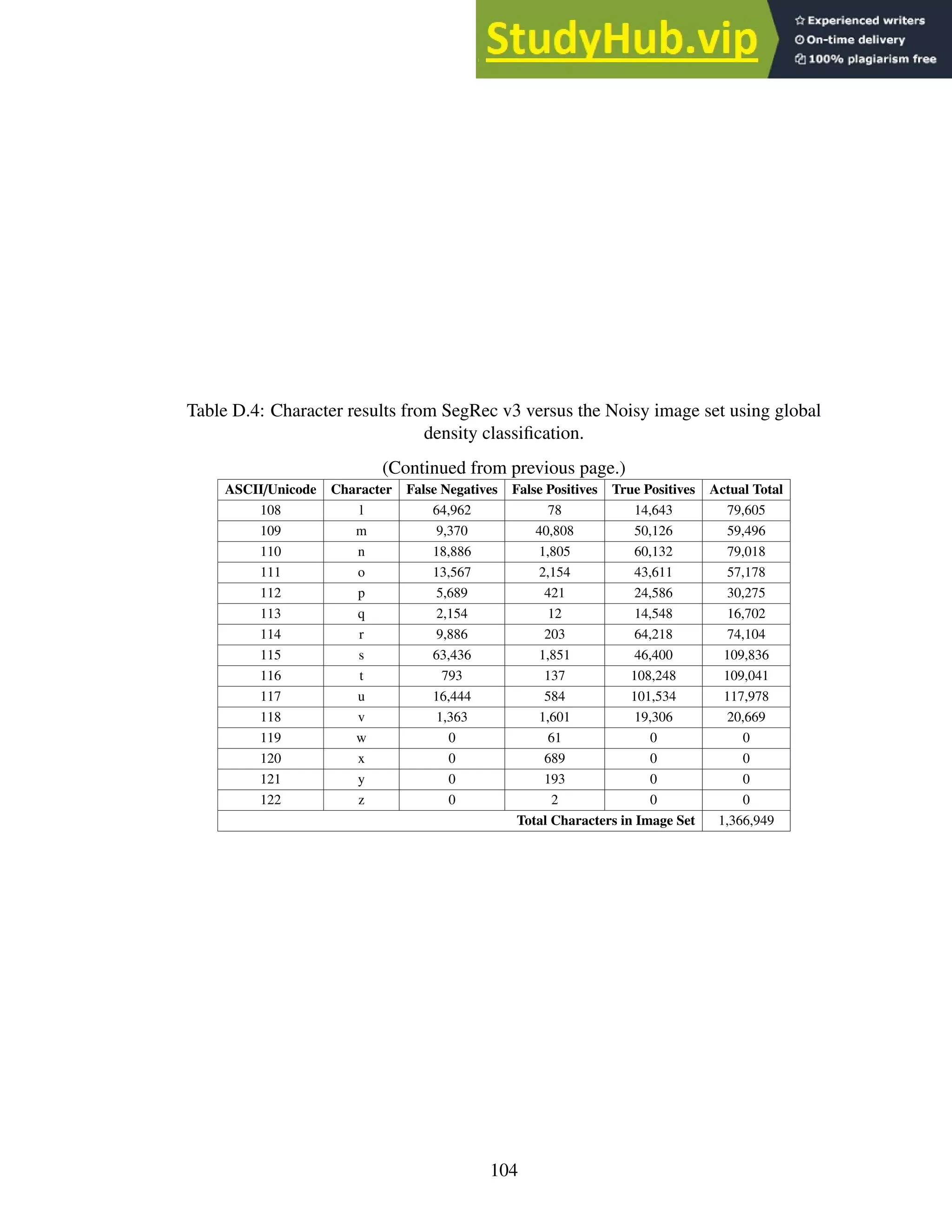


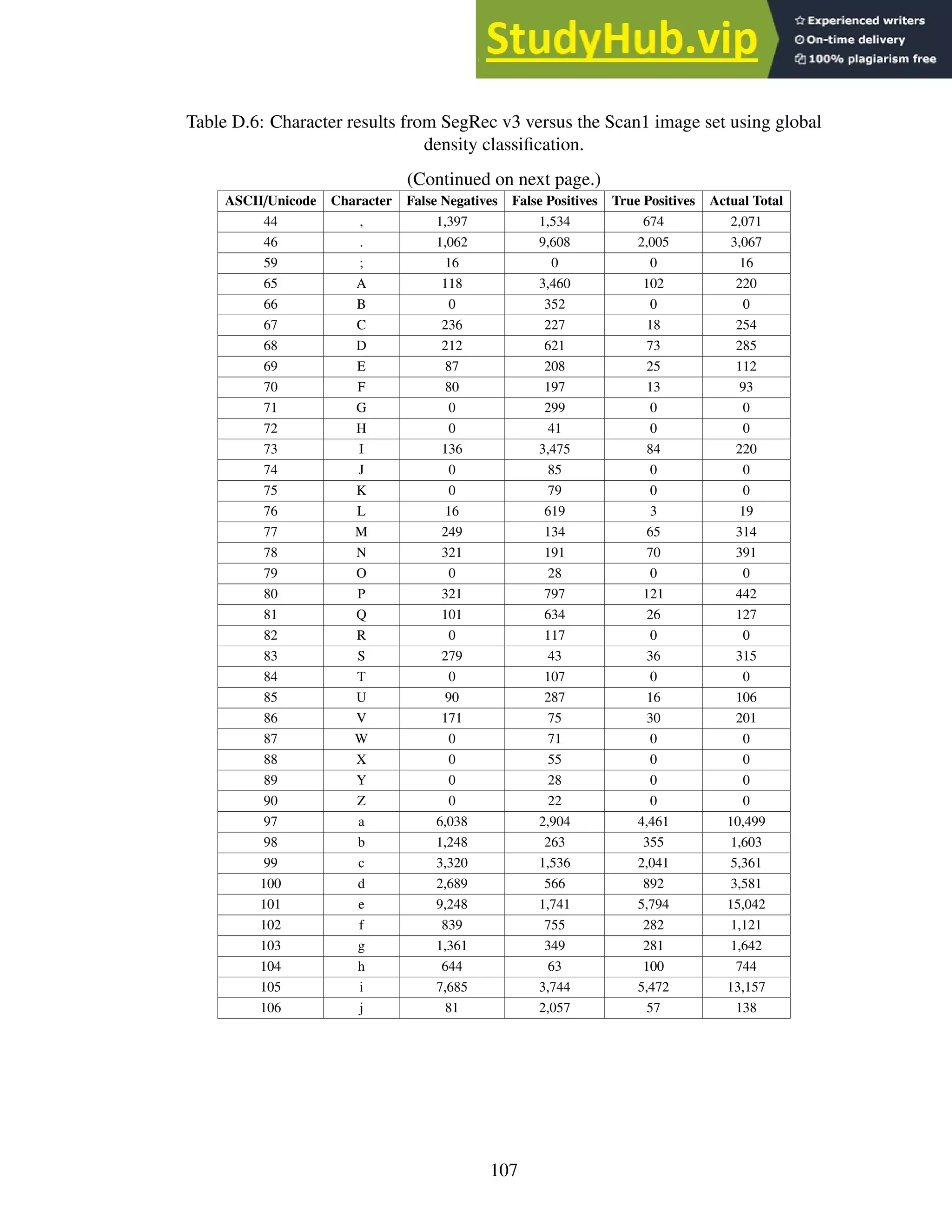

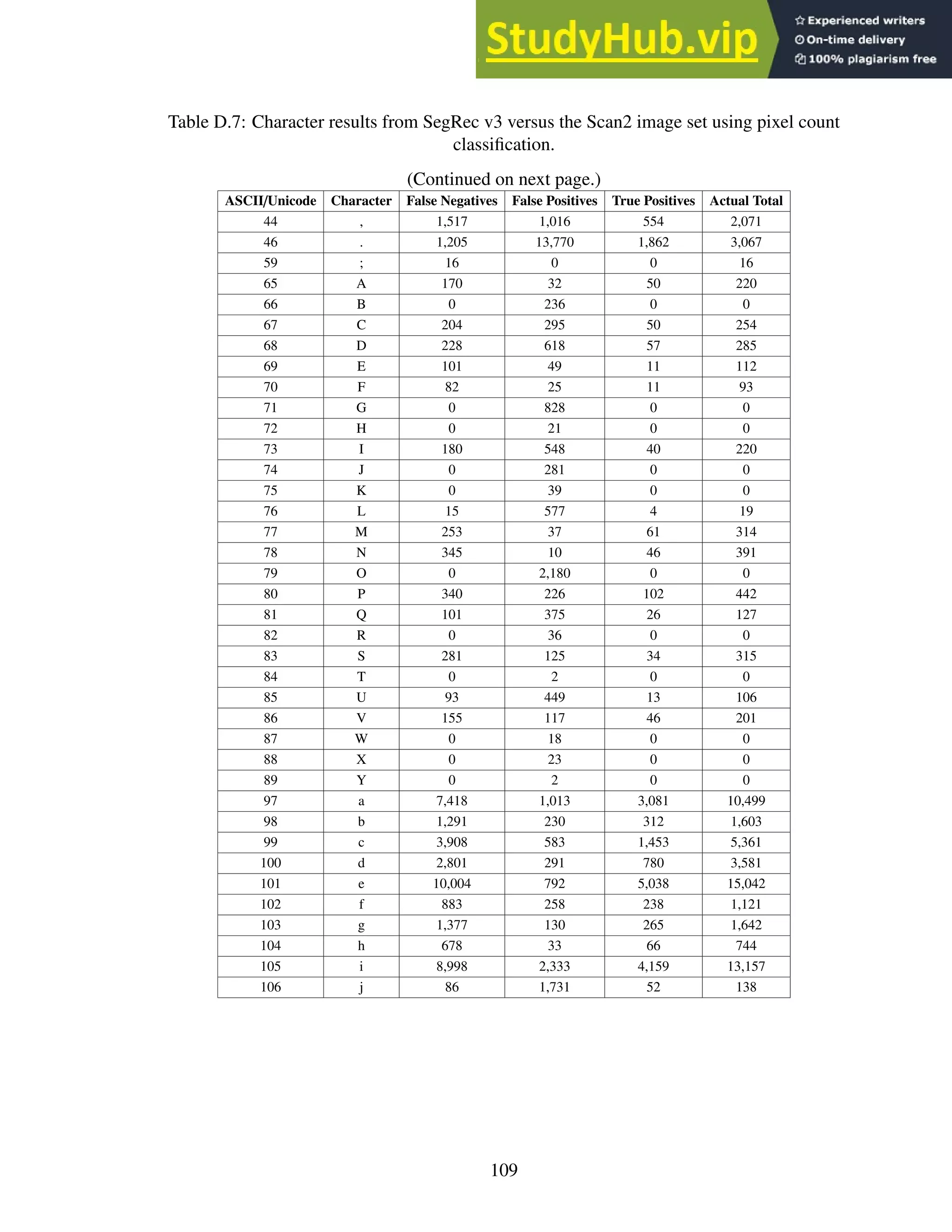


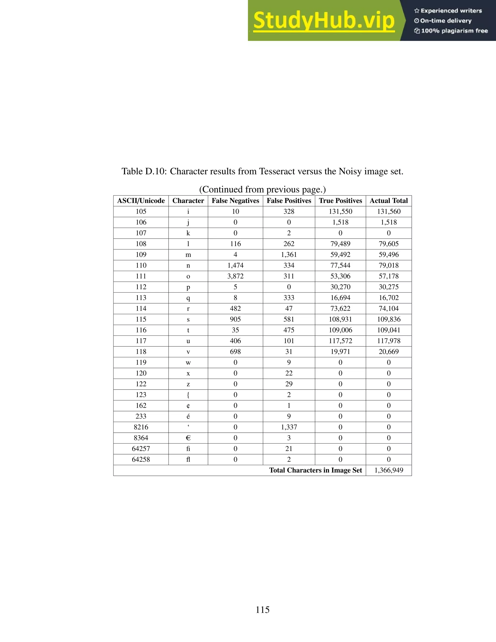
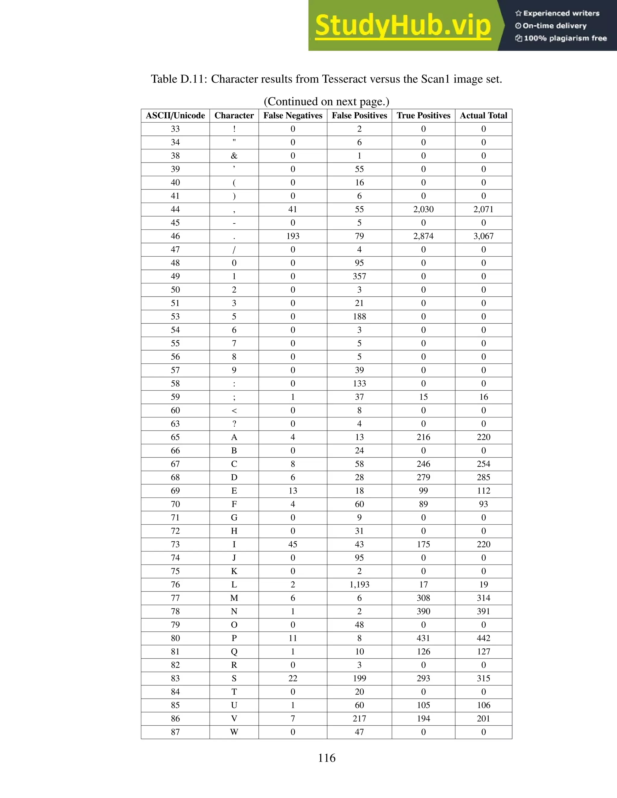
![Table D.11: Character results from Tesseract versus the Scan1 image set.
(Continued from previous page.)
ASCII/Unicode Character False Negatives False Positives True Positives Actual Total
89 Y 0 1 0 0
90 Z 0 2 0 0
91 [ 0 19 0 0
92 0 3 0 0
93 ] 0 49 0 0
95 _ 0 9 0 0
97 a 349 167 10,150 10,499
98 b 37 16 1,566 1,603
99 c 220 590 5,141 5,361
100 d 42 21 3,539 3,581
101 e 1,796 265 13,246 15,042
102 f 174 12 947 1,121
103 g 227 36 1,415 1,642
104 h 10 83 734 744
105 i 713 727 12,444 13,157
106 j 7 256 131 138
107 k 0 6 0 0
108 l 1,241 199 6,676 7,917
109 m 84 161 5,979 6,063
110 n 226 264 7,482 7,708
111 o 377 1,014 5,316 5,693
112 p 41 13 2,732 2,773
113 q 23 247 1,743 1,766
114 r 306 59 7,049 7,355
115 s 950 61 10,151 11,101
116 t 1,362 201 9,470 10,832
117 u 293 426 11,687 11,980
118 v 213 73 1,818 2,031
119 w 0 17 0 0
120 x 0 46 260 260
121 y 0 14 0 0
122 z 0 28 0 0
123 { 0 1 0 0
124 | 0 2 0 0
125 } 0 10 0 0
126 ~ 0 1 0 0
187 » 0 4 0 0
233 é 0 1 0 0
8212 — 0 1 0 0
8216 ‘ 0 82 0 0
8217 ’ 0 8 0 0
8220 “ 0 8 0 0
8221 ” 0 5 0 0
64257 fi 0 45 0 0
64258 fl 0 8 0 0
Total Characters in Image Set 136,620
117](https://image.slidesharecdn.com/anopticalcharacterrecognitionengineforgraphicalprocessingunits-230805215723-24ac1bd2/75/An-Optical-Character-Recognition-Engine-For-Graphical-Processing-Units-130-2048.jpg)
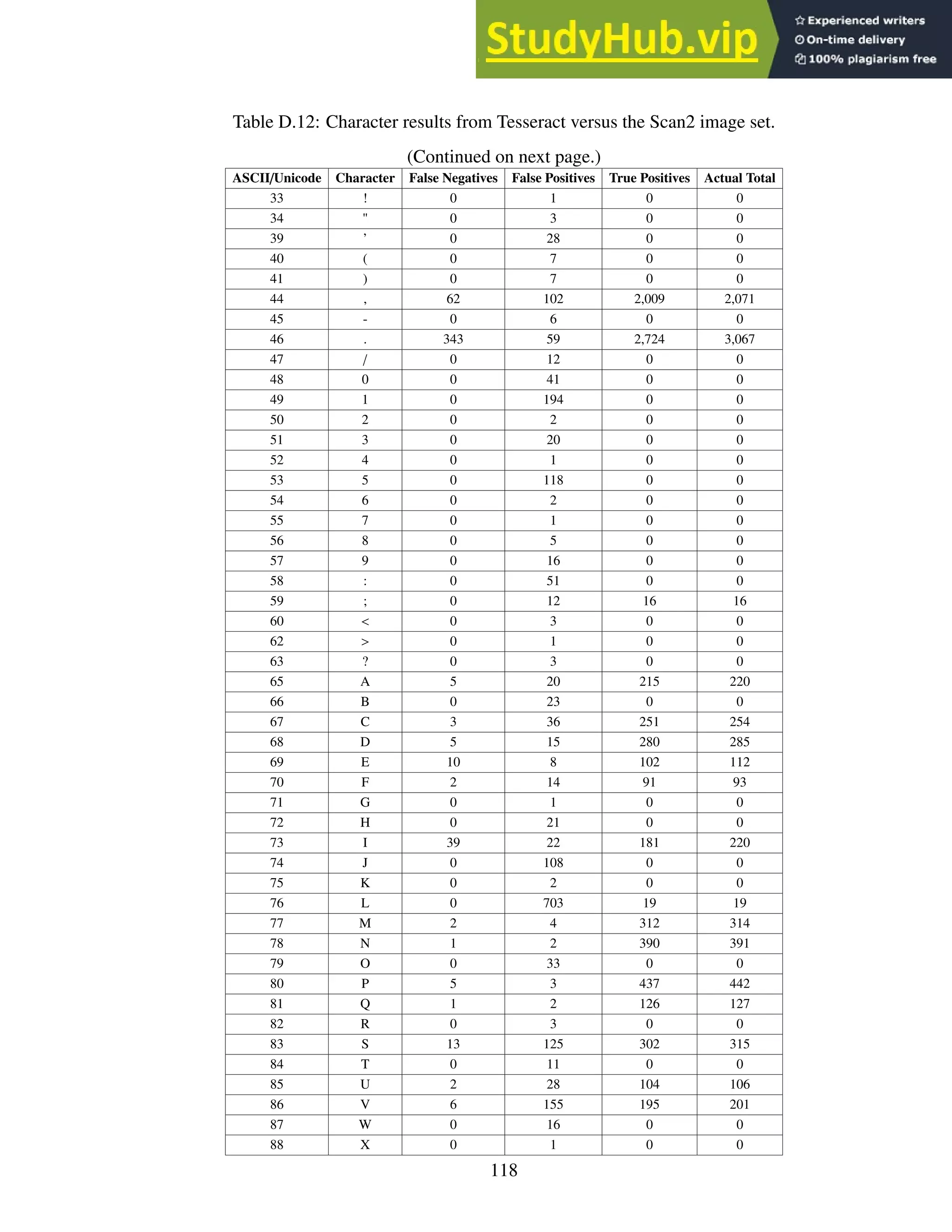
![Table D.12: Character results from Tesseract versus the Scan2 image set.
(Continued from previous page.)
ASCII/Unicode Character False Negatives False Positives True Positives Actual Total
89 Y 0 1 0 0
90 Z 0 1 0 0
91 [ 0 6 0 0
92 0 5 0 0
93 ] 0 64 0 0
95 _ 0 4 0 0
97 a 162 183 10,337 10,499
98 b 18 10 1,585 1,603
99 c 162 404 5,199 5,361
100 d 15 15 3,566 3,581
101 e 1,176 275 13,866 15,042
102 f 87 15 1,034 1,121
103 g 138 30 1,504 1,642
104 h 5 60 739 744
105 i 586 406 12,571 13,157
106 j 2 276 136 138
107 k 0 5 0 0
108 l 752 143 7,165 7,917
109 m 36 139 6,027 6,063
110 n 173 160 7,535 7,708
111 o 329 612 5,364 5,693
112 p 22 17 2,751 2,773
113 q 12 149 1,754 1,766
114 r 172 50 7,183 7,355
115 s 633 65 10,468 11,101
116 t 825 149 10,007 10,832
117 u 166 196 11,814 11,980
118 v 142 54 1,889 2,031
119 w 0 8 0 0
120 x 1 36 259 260
121 y 0 11 0 0
122 z 0 15 0 0
123 { 0 1 0 0
124 | 0 2 0 0
125 } 0 6 0 0
126 ~ 0 5 0 0
163 £ 0 1 0 0
187 » 0 4 0 0
233 é 0 2 0 0
8212 — 0 1 0 0
8216 ‘ 0 116 0 0
8217 ’ 0 9 0 0
8220 “ 0 3 0 0
8221 ” 0 1 0 0
8364 € 0 1 0 0
64257 fi 0 36 0 0
64258 fl 0 12 0 0
Total Characters in Image Set 136,620
119](https://image.slidesharecdn.com/anopticalcharacterrecognitionengineforgraphicalprocessingunits-230805215723-24ac1bd2/75/An-Optical-Character-Recognition-Engine-For-Graphical-Processing-Units-132-2048.jpg)
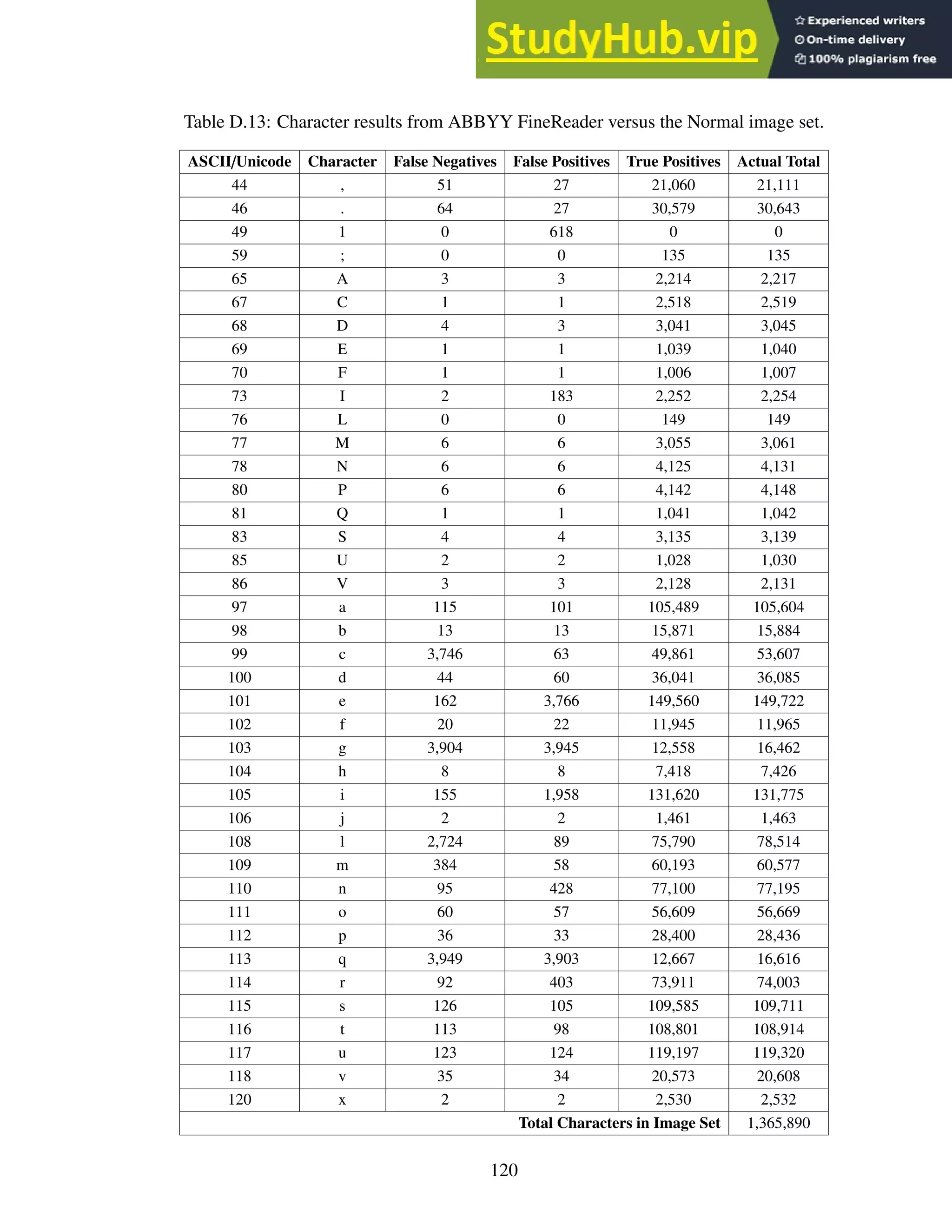


![Table D.15: Character results from ABBYY FineReader versus the Scan1 image set.
(Continued on next page.)
ASCII/Unicode Character False Negatives False Positives True Positives Actual Total
33 ! 0 22 0 0
34 " 0 2 0 0
39 ’ 0 24 0 0
41 ) 0 3 0 0
44 , 8 45 2,063 2,071
45 - 0 9 0 0
46 . 21 663 3,046 3,067
47 / 0 4 0 0
49 1 0 79 0 0
51 3 0 2 0 0
53 5 0 5 0 0
58 : 0 76 0 0
59 ; 0 30 16 16
60 < 0 1 0 0
62 > 0 3 0 0
65 A 0 0 220 220
67 C 15 2 239 254
68 D 3 0 282 285
69 E 6 1 106 112
70 F 1 3 92 93
71 G 0 14 0 0
72 H 0 4 0 0
73 I 4 31 216 220
74 J 0 4 0 0
75 K 0 4 0 0
76 L 0 67 19 19
77 M 1 3 313 314
78 N 7 2 384 391
79 O 0 2 0 0
80 P 5 2 437 442
81 Q 0 0 127 127
82 R 0 1 0 0
83 S 1 2 314 315
84 T 0 4 0 0
85 U 1 7 105 106
86 V 0 0 201 201
87 W 0 1 0 0
93 ] 0 11 0 0
94 ˆ 0 2 0 0
95 _ 0 1 0 0
97 a 75 109 10,424 10,499
98 b 13 16 1,590 1,603
99 c 360 157 5,001 5,361
100 d 11 12 3,570 3,581
123](https://image.slidesharecdn.com/anopticalcharacterrecognitionengineforgraphicalprocessingunits-230805215723-24ac1bd2/75/An-Optical-Character-Recognition-Engine-For-Graphical-Processing-Units-136-2048.jpg)

![Table D.16: Character results from ABBYY FineReader versus the Scan2 image set.
(Continued on next page.)
ASCII/Unicode Character False Negatives False Positives True Positives Actual Total
33 ! 0 17 0 0
39 ’ 0 11 0 0
40 ( 0 1 0 0
42 * 0 2 0 0
44 , 11 65 2,060 2,071
45 - 0 22 0 0
46 . 59 374 3,008 3,067
47 / 0 8 0 0
49 1 0 28 0 0
51 3 0 3 0 0
53 5 0 1 0 0
58 : 0 47 0 0
59 ; 0 19 16 16
62 > 0 1 0 0
65 A 0 0 220 220
66 B 0 1 0 0
67 C 9 0 245 254
68 D 0 0 285 285
69 E 4 1 108 112
70 F 0 0 93 93
71 G 0 7 0 0
72 H 0 8 0 0
73 I 6 23 214 220
74 J 0 7 0 0
75 K 0 1 0 0
76 L 0 12 19 19
77 M 1 3 313 314
78 N 10 0 381 391
80 P 2 1 440 442
81 Q 0 0 127 127
83 S 0 2 315 315
85 U 0 7 106 106
86 V 0 0 201 201
87 W 0 1 0 0
93 ] 0 4 0 0
95 _ 0 1 0 0
97 a 40 122 10,459 10,499
98 b 4 27 1,599 1,603
99 c 339 74 5,022 5,361
100 d 6 9 3,575 3,581
101 e 180 341 14,862 15,042
102 f 1 7 1,120 1,121
103 g 15 24 1,627 1,642
125](https://image.slidesharecdn.com/anopticalcharacterrecognitionengineforgraphicalprocessingunits-230805215723-24ac1bd2/75/An-Optical-Character-Recognition-Engine-For-Graphical-Processing-Units-138-2048.jpg)
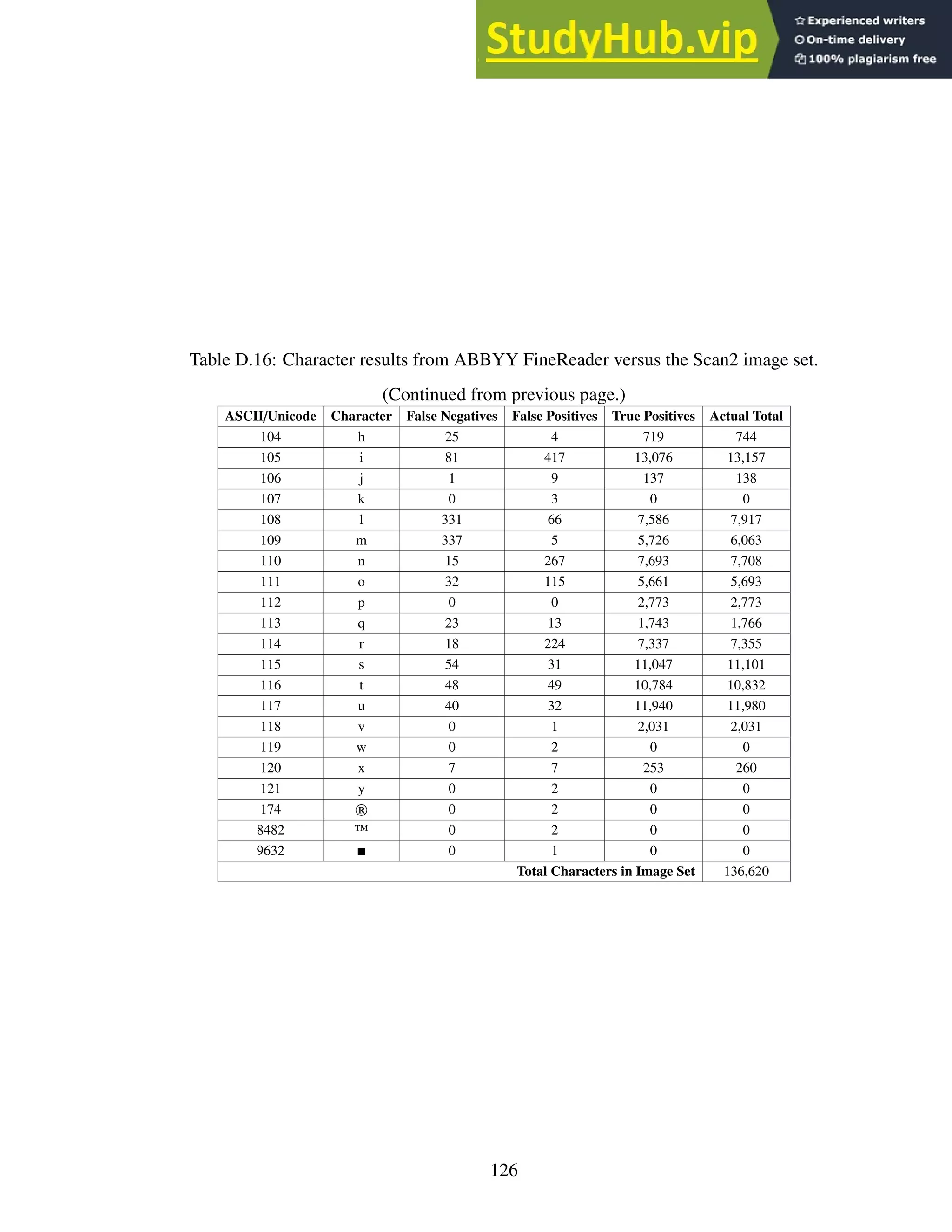

![Table D.18: Character results from OmniPage Ultimate versus the Noisy image set.
(Continued on next page.)
ASCII/Unicode Character False Negatives False Positives True Positives Actual Total
33 ! 0 13 0 0
37 % 0 2 0 0
38 0 4 0 0
39 ’ 0 15 0 0
40 ( 0 6 0 0
41 ) 0 46 0 0
44 , 38 52 21,116 21,154
45 - 0 16 0 0
46 . 111 33 30,266 30,377
47 / 0 3 0 0
49 1 0 24 0 0
52 4 0 2 0 0
53 5 0 4 0 0
58 : 0 5 0 0
59 ; 4 2 158 162
61 = 0 6 0 0
63 ? 0 3 0 0
65 A 1 4 2,103 2,104
66 B 0 22 0 0
67 C 231 11 2,240 2,471
68 D 22 15 3,015 3,037
69 E 9 6 974 983
70 F 6 13 979 985
71 G 0 288 0 0
72 H 0 9 0 0
73 I 10 10 2,365 2,375
74 J 0 5 0 0
76 L 3 5 148 151
77 M 1 4 3,048 3,049
78 N 16 5 4,177 4,193
79 O 0 15 0 0
80 P 15 24 4,091 4,106
81 Q 5 2 1,005 1,010
82 R 0 1 0 0
83 S 22 6 3,072 3,094
84 T 0 5 0 0
85 U 45 1 918 963
86 V 11 2 2,169 2,180
87 W 0 1 0 0
93 ] 0 4 0 0
94 ˆ 0 3 0 0
95 _ 0 15 0 0
128](https://image.slidesharecdn.com/anopticalcharacterrecognitionengineforgraphicalprocessingunits-230805215723-24ac1bd2/75/An-Optical-Character-Recognition-Engine-For-Graphical-Processing-Units-141-2048.jpg)
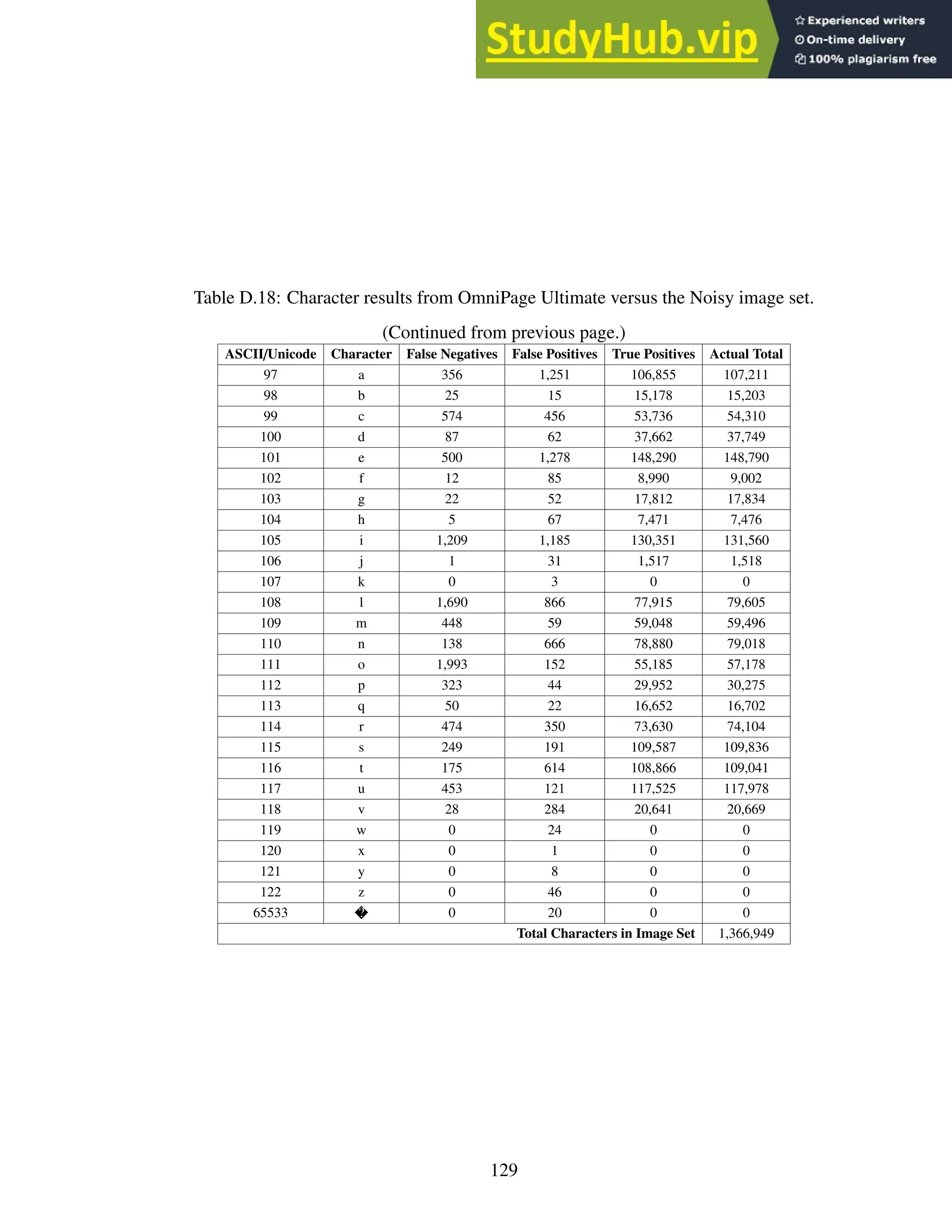
![Table D.19: Character results from OmniPage Ultimate versus the Scan1 image set.
(Continued on next page.)
ASCII/Unicode Character False Negatives False Positives True Positives Actual Total
33 ! 0 2 0 0
38 0 2 0 0
39 ’ 0 20 0 0
40 ( 0 5 0 0
41 ) 0 8 0 0
42 * 0 3 0 0
43 + 0 1 0 0
44 , 8 13 2,063 2,071
46 . 9 170 3,058 3,067
47 / 0 3 0 0
49 1 0 6 0 0
50 2 0 1 0 0
51 3 0 8 0 0
52 4 0 2 0 0
58 : 0 28 0 0
59 ; 2 8 14 16
61 = 0 4 0 0
65 A 0 6 220 220
66 B 0 6 0 0
67 C 5 14 249 254
68 D 5 2 280 285
69 E 17 0 95 112
70 F 5 4 88 93
71 G 0 5 0 0
72 H 0 7 0 0
73 I 12 16 208 220
74 J 0 1 0 0
75 K 0 5 0 0
76 L 2 113 17 19
77 M 5 7 309 314
78 N 4 5 387 391
79 O 0 4 0 0
80 P 5 5 437 442
81 Q 0 0 127 127
82 R 0 5 0 0
83 S 2 10 313 315
84 T 0 5 0 0
85 U 7 10 99 106
86 V 0 0 201 201
87 W 0 3 0 0
93 ] 0 27 0 0
95 _ 0 1 0 0
130](https://image.slidesharecdn.com/anopticalcharacterrecognitionengineforgraphicalprocessingunits-230805215723-24ac1bd2/75/An-Optical-Character-Recognition-Engine-For-Graphical-Processing-Units-143-2048.jpg)

![Table D.20: Character results from OmniPage Ultimate versus the Scan2 image set.
(Continued on next page.)
ASCII/Unicode Character False Negatives False Positives True Positives Actual Total
33 ! 0 4 0 0
38 0 3 0 0
39 ’ 0 5 0 0
40 ( 0 3 0 0
41 ) 0 8 0 0
44 , 8 5 2,063 2,071
45 - 0 3 0 0
46 . 8 96 3,059 3,067
48 0 0 1 0 0
49 1 0 3 0 0
51 3 0 9 0 0
58 : 0 21 0 0
59 ; 1 1 15 16
61 = 0 9 0 0
65 A 2 2 218 220
66 B 0 10 0 0
67 C 2 4 252 254
68 D 4 1 281 285
69 E 19 0 93 112
70 F 4 1 89 93
71 G 0 6 0 0
72 H 0 8 0 0
73 I 12 9 208 220
74 J 0 5 0 0
75 K 0 2 0 0
76 L 0 20 19 19
77 M 6 2 308 314
78 N 3 3 388 391
79 O 0 5 0 0
80 P 0 4 442 442
81 Q 0 0 127 127
83 S 0 10 315 315
84 T 0 1 0 0
85 U 1 3 105 106
86 V 0 0 201 201
87 W 0 1 0 0
88 X 0 2 0 0
93 ] 0 21 0 0
132](https://image.slidesharecdn.com/anopticalcharacterrecognitionengineforgraphicalprocessingunits-230805215723-24ac1bd2/75/An-Optical-Character-Recognition-Engine-For-Graphical-Processing-Units-145-2048.jpg)
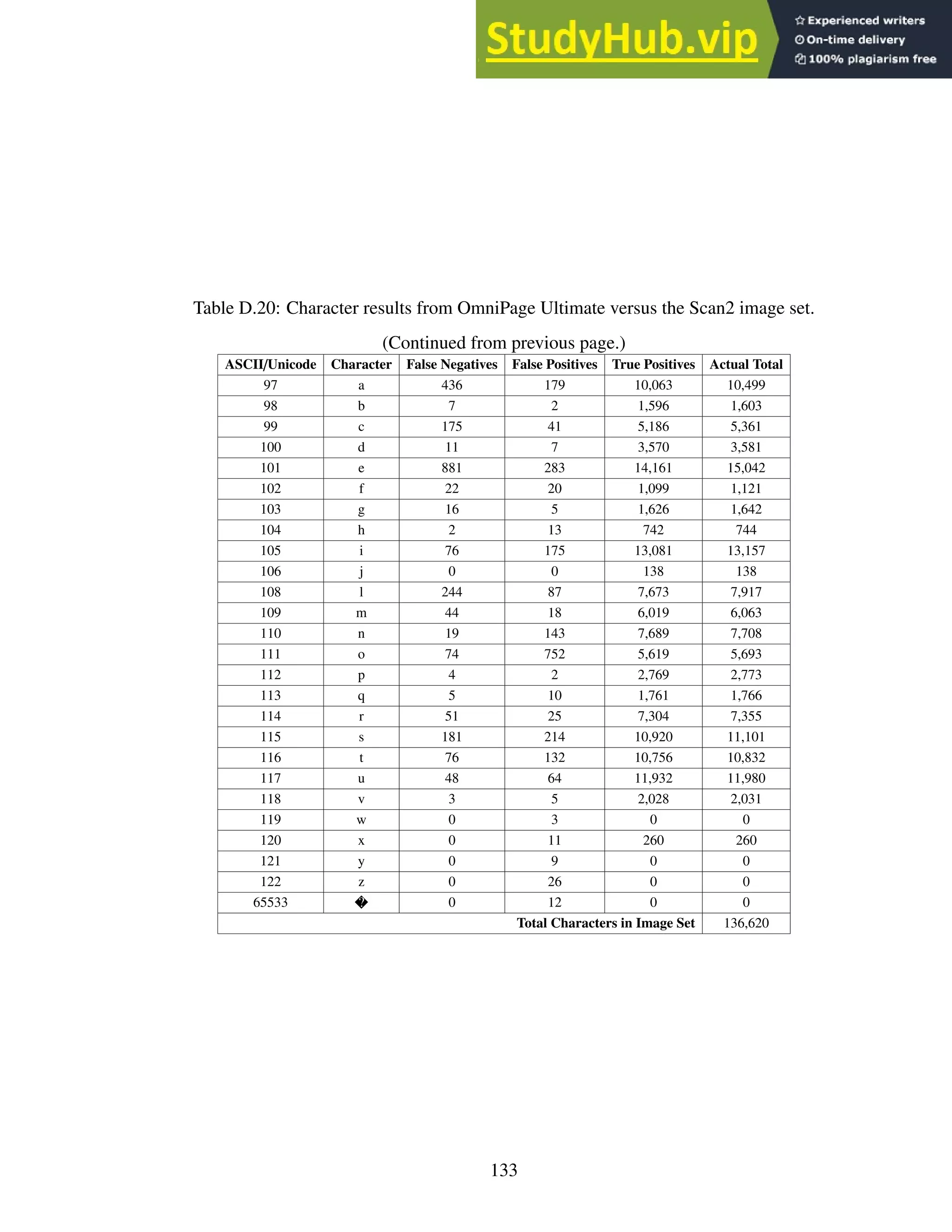
![Bibliography
[1] Dibco 2014. http://users.iit.demokritos.gr/~kntir/HDIBCO2014/
index.html. Accessed: 2015-08-03.
[2] ABBYY. About ABBYY. https://www.abbyy.com/en-us/company/key-facts/, October
2016.
[3] A. S. Abutableb. Automatic thresholding of gray-level pictures using two-
dimensional entropy. Computer Vision, Graphics, and Image Processing, 47:22–32,
1989.
[4] Adnan Amin and Sue Wu. A robust system for thresholding and skew detection
in mixed text/graphics documents. International Journal of Image and Graphics,
5(2):247–265, Apr 2005.
[5] Itay Bar-Yosef, Alik Mokeichev, Klara Kedem, Itshak Dinstein, and Uri Ehrlich.
Adaptive shape prior for recognition and variational segmentation of degraded his-
torical characters. Pattern Recognition, 42(12):3348–3354, Dec 2009.
[6] Junior Barrera, Marcel Brun, Routo Terada, and Edward R. Dougherty. Boosting
OCR classifier by optimal edge noise filtering. Computational Imaging and Vision,
18(9):371–380, 2002.
[7] Subhadip Basu, Nibaran Das, Ram Sarkar, Mahantapas Kundu, Mita Nasipuri, and
Dipak Kumar Basu. A hierarchical approach to recognition of handwritten bangla
characters. Pattern Recognition, 42(7):1467–1484, July 2009.
[8] C. I. Chang, Y. Du, J. Wang, S. M. Guo, and P. D. Thouin. Survey and comparative
analysis of entropy and relative entropy thresholding techniques. IEEE Proceedings
Vision, Image and Signal Processing, 153(6), Dec 2006.
[9] Xin Chen, Yuefang Gao, and Zhonghong Huang. Cuda-accelerated fast sauvola’s
method on kepler architecture. Multimedia Tools and Applications, pages 1–12, 2014.
[10] John Cheng, Max Grossman, and Ty McKercher. Professional CUDA C Program-
ming. John Wiley and Sons, Inc., 2014.
[11] E.E. Fournier D’Albe. On a type-reading optophone. Proceedings of the Royal Society
of London A: Mathematical, Physical and Engineering Sciences, 90(619):373–375,
May 1914.
[12] A. K. Das and B. Chanda. A fast algorithm for skew detection of document images
using morphology. International Journal on Document Analysis and Recognition,
4(2):109–114, 2001.
[13] Raphael Finkel. Multilingual ocr program. personal communication.
134](https://image.slidesharecdn.com/anopticalcharacterrecognitionengineforgraphicalprocessingunits-230805215723-24ac1bd2/75/An-Optical-Character-Recognition-Engine-For-Graphical-Processing-Units-147-2048.jpg)
![[14] Herbert Freeman. On the encoding of arbitrary geometric configurations. IRE Trans-
actions on Electronic Computers, EC-10(2):260–268, June 1961.
[15] B. Gatos, K. Ntirogiannis, and I. Pratikakis. Icdar 2009 document image binarization
contest (dibco 2009). pages 1375–1382, July 2009.
[16] Emanuel Goldberg. Statistical machine, Dec 1931. US Patent 1,838,389.
[17] Amara Graps. An introduction to wavelets. IEEE Computation Science and Engi-
neering, 2(2), 1995.
[18] Josh Hershberger and Jack Snoeyink. Speeding up the douglas-peucker line-
simplification algorithm. 1992.
[19] L. Hertz and R. W. Schafer. Multilevel thresholding using edge matching. Computer
Vision, Graphics, and Image Processing, 44:279–295, 1988.
[20] Robert Hummel. Image enhancement by histogram transformation. Computer Graph-
ics and Image Processing, 6(2):184–195, April 1977.
[21] J. N. Kapur, P. K. Sahoo, and A. K. C. Wong. A new method for gray-level picture
thresholding using the entropy of the histogram. Computer Vision, Graphics, and
Image Processing, 29(3):273–285, Mar 1985.
[22] D.J. Ketcham, R.W. Lowe, and J.W. Weber. Real-time image enhancement tech-
niques. Image Processing, 74, July 1976.
[23] Koichi Kise, Akinori Sato, and Motoi Iwata. Segmentation of page images using the
area voronoi diagram. Computer Vision and Image Understanding, 70(3):370–382,
June 1998.
[24] Donald E. Knuth. The concept of a meta-font. Visible Language, 16:3–27, 1982.
[25] Karen Kukich. Techniques for automatically correcting words in text. ACM Comput.
Surv., 24(4):377–439, Dec 1992.
[26] C. Vasantha Lakshmi, Sarika Singh, Ritu Jain, and C. Patvardhan. A novel approach
to skeletonization for multi-font ocr applications. Lecture Notes in Computer Science,
5909:393–399, 2009.
[27] S. Lawson and J. Zhu. Image compression using wavelets and jpeg2000: a tutorial.
Electronics and Communication Engineering Journal, pages 112–121, June 2002.
[28] Sabri A. Mahmoud and Ashraf S. Mahmoud. Arabic character recognition using
modified Fourier spectrum (MFS) vs. Fourier descriptors. Cybernetics and Systems,
40(3):189–210, Mar 2009.
[29] Manjunath Aradhya V. N., Hemantha Kumar G., and Shivakumara P. Skew detec-
tion technique for binary document images based on Hough transform. International
Journal of Information and Communication Engineering, March:498–504, Mar 2007.
135](https://image.slidesharecdn.com/anopticalcharacterrecognitionengineforgraphicalprocessingunits-230805215723-24ac1bd2/75/An-Optical-Character-Recognition-Engine-For-Graphical-Processing-Units-148-2048.jpg)
![[30] M. J. Nassiri, A. Vafaei, and A. Monadjemi. Texture feature extraction using Slant-
Hadamard transform. World Academy of Science, Engineering and Technology, 17,
2006.
[31] W. Niblack. An Introduction to Digital Image Processing. Prentice-Hall, Englewood
Cliffs, NJ.
[32] K. Ntirogiannis, B. Gatos, and I. Pratikakis. Icfhr2014 competition on handwritten
document image binarization (h-dibco 2014). pages 809–813, Sept 2014.
[33] Nuance. Nuance fast facts. http://www.nuance.com/company/company-overview/fast-
facts/index.htm, October 2016.
[34] NVIDIA. Nvidia CUDA C Programming Guide v7.0. http://docs.nvidia.com/cuda/pdf/
CUDA_C_Programming_Guide.pdf, March 2015.
[35] NVIDIA. Nvidia Parallel Thread Execution ISA v4.3.
http://docs.nvidia.com/cuda/parallel-thread-execution/, September 2015.
[36] NVIDIA. Nvidia Profiler User’s Guide. http://docs.nvidia.com/cuda/profiler-users-
guide/, September 2015.
[37] N. Otsu. A thresholding selection method from gray-scale histogram. IEEE Transac-
tions on System, Man, and Cybernetics, 9:62–66, 1979.
[38] S.M. Pizer. Intensity mappings for the display of medical images. Functional Map-
ping of Organ Systems and Other Computer Topics, 1981.
[39] Stephen M. Pizer, E. Philip Amburn, John D. Austin, Robert Cromartie, Ari
Geselowitz, Trey Greer, Bart ter Haar Romeny, John B. Zimmerman, and Karel
Zuiderveld. Adaptive histogram equalization and its variations. Computer Vision,
Graphics, and Image Processing, 39:355–368, 1987.
[40] I. Pratikakis, B. Gatos, and K. Ntirogiannis. H-dibco 2010 - handwritten document
image binarization competition. pages 727–732, Nov 2010.
[41] I. Pratikakis, B. Gatos, and K. Ntirogiannis. Icdar 2011 document image binarization
contest (dibco 2011). pages 1506–1510, Sept 2011.
[42] I. Pratikakis, B. Gatos, and K. Ntirogiannis. Icfhr 2012 competition on handwritten
document image binarization (h-dibco 2012). pages 817–822, Sept 2012.
[43] I. Pratikakis, B. Gatos, and K. Ntirogiannis. Icdar 2013 document image binarization
contest (dibco 2013). pages 1471–1476, Aug 2013.
[44] Stephen V. Rice, Frank R. Jenkins, and Thomas A. Nartker. The fourth annual test of
ocr accuracy, technical report 95-03. July 1995.
[45] J. Sauvola and M. Pietikäinen. Adaptive document image binarization. Pattern Recog-
nition, 33(2):225–236, Feb 2000.
136](https://image.slidesharecdn.com/anopticalcharacterrecognitionengineforgraphicalprocessingunits-230805215723-24ac1bd2/75/An-Optical-Character-Recognition-Engine-For-Graphical-Processing-Units-149-2048.jpg)
![[46] M. I. Sezan. A peak detection algorithm and its application to histogram-based im-
age data reduction. Computer Vision, Graphics, and Image Processing, 49(1):36–51,
1990.
[47] Faisal Shafait, Daniel Keysers, and Thomas M. Breuel. Performance evaluation and
benchmarking of six page segmentation algorithms. IEEE Transactions on Pattern
Analysis and Machine Intelligence, 30(6):941–954, June 2008.
[48] N. Shanthi and K. Duraiswamy. A novel SVM-based handwritten Tamil character
recognition system. Pattern Analysis and Applications, 13(2):173–180, May 2010.
[49] Brij Mohan Singh, Rashi Nitin Gupta, Ankush Mittal, and Debashish Ghosh. Paral-
lel implementation of devanagari text line and word segmentation approach on gpu.
International Journal of Computer Applications, 24(9):7–14, June 2011.
[50] Brij Mohan Singh, Rahul Sharmal, Ankush Mittal, and Debashish Ghosh. Parallel
implementation of niblack’s binarization approach on cuda. International Journal of
Computer Applications, 32(2):22–27, October 2011.
[51] Brij Mohan Singh, Rahul Sharmal, Ankush Mittal, and Debashish Ghosh. Parallel
implementation of Otsu’s binarization approach on cuda. International Journal of
Computer Applications, 32(2):16–21, October 2011.
[52] Brij Mohan Singh, Rahul Sharmal, Ankush Mittal, and Debashish Ghosh. Parallel
implementation of Souvola’s binarization approach on cuda. International Journal of
Computer Applications, 32(2):28–33, October 2011.
[53] Ray Smith. An overview of the Tesseract OCR engine. Proc. of ICDAR 2007, pages
629–633, 2007.
[54] Eric J. Sollnitz, Tony D. DeRose, and David H. Salesin. Wavelets for computer graph-
ics: A primer, part 1. IEEE Computer Graphics and Applications, 15(3):76–84, May
1995.
[55] J. M. White and G. D. Rohrer. Image thresholding for optical character recognition
and other applications requiring character image extraction. Develop, 27(4):400–411,
July 1983.
[56] Abdelwahab Zramdini and Rolf Ingold. Optical font recognition from projection
profiles. Electronic Publishing, 6(3):249–260, Sep 1993.
137](https://image.slidesharecdn.com/anopticalcharacterrecognitionengineforgraphicalprocessingunits-230805215723-24ac1bd2/75/An-Optical-Character-Recognition-Engine-For-Graphical-Processing-Units-150-2048.jpg)


This dissertation investigates building an optical character recognition (OCR) engine for graphical processing units (GPUs). It describes Jeremy Reed's doctoral dissertation from the University of Kentucky in 2016. The dissertation introduces basic OCR and GPU concepts. It then describes in detail the SegRec algorithm developed by the author for segmenting and recognizing characters on a GPU. Evaluation results comparing SegRec to other OCR engines are provided. The dissertation concludes by discussing limitations and opportunities for improving SegRec and developing it into a full-featured OCR system.