This document is a thesis submitted by Ruaan van Zyl to the University of Stellenbosch in fulfillment of the requirements for a Doctor of Philosophy degree. The thesis proposes Bayesian control charts based on predictive distributions for monitoring processes with unknown parameters. It develops Bayesian control charts for several common distributions, including the normal, exponential, and piecewise exponential models. The thesis contains 8 chapters that describe the Bayesian methodology, derive appropriate prior distributions, and demonstrate the proposed control charts through simulation studies.


![2.4 Reference and Probability-Matching Priors
Note: The ordering {γ; (σ2
1, σ2
2, . . . , σ2
¨m)} means that the coefficient of variation is
the most important parameter while the ¨m variance components are of equal im-
portance, but not as important as γ. Also, if ¨m = 1, the above equation simplifies
to the reference prior obtained by Berger, Liseo, and Wolpert (1999).
Proof. The proof is given in the Mathematical Appendices to this chapter.
2.4.2. Probability-matching Priors
The reference prior algorithm is but one way to obtain a useful non-informative prior.
Another type of non-informative prior is the probability-matching prior. This prior
has good frequentist properties.
As mentioned in the introduction p (θ) is a probability-matching prior for θ =
[γ, σ2
1, σ2
2, . . . , σ2
¨m] the vector of unknown parameters, if the following differential
equation is satisfied:
¨m+1
α=1
∂
∂θα
{Υα (θ) p (θ)} = 0
where
Υ (θ) =
F−1
(θ) t (θ)
t (θ) F−1 (θ) t (θ)
= Υ1 (θ) Υ2 (θ) · · · Υ¨m+1 (θ)
and
t (θ) = ∂
∂θ1
t (θ) ∂
∂θ2
t (θ) · · · ∂
∂θ ¨m+1
t (θ) .
t (θ) is a function of θ and F−1
(θ) is the inverse of the Fisher information matrix.
Theorem 2.3. The probability-matching prior for the coefficient of variation γ and
the variance components is given by
27](https://image.slidesharecdn.com/328932de-d899-482b-a718-5e10677662e8-160621144849/85/thesis-35-320.jpg)


![2.6 Additional Details on Priors and Methods Used
interest in the sufficient statistics ¯Xi and Si these can be simulated directly, namely
¯Xi ∼ N µi,
σ2
i
n
and S2
i ∼
σ2
i χ2
n−1
n−1
.
The simulated ¯Xi and S2
i (i = 1, 2, . . . , ¨m) values are then substituted in the condi-
tional posterior distributions p (σ1, σ2, . . . , σ¨m|γ, data) and p (γ|σ1, σ2, . . . , σ¨m) (Equa-
tions (2.4) and (2.5)). By using the conditional posterior distributions and Gibbs
sampling the unconditional posterior distribution p (γ|data) can be obtained. A
confidence interval for γ will be calculated as follows:
Simulate l = 10, 000 values of γ and sort the values in ascending order ˜γ(1) ≤ ˜γ(2) ≤
· · · ≤ ˜γ(l).
Let K1 = α
2
l and K2 = 1 − α
2
l where [a] denotes the largest integer not greater
than a. ˜γ(K1), ˜γ(K2) is then a 100 (1 − α) % Bayesian confidence interval for γ.
By repeating the procedure for R = 3, 000 datasets it is found that the 3, 000
95% Bayesian confidence intervals (α = 0.05) cover the parameter γ = 0.075 in
2, 841 cases. An estimate of the frequentist probability of coverage is therefore
P ˜γ(K1) < γ < ˜γ(K2) = 0.9470. Also P γ ≤ ˜γ(K1) = 0.00217 and P γ ≥ ˜γ(K2) =
0.0313.
2.6. Additional Details on Priors and Methods Used
Upon suggestion from external assessor further details on priors and methods used
in this Chapter and throughout the thesis is provided in this section.
2.6.1. Reference Priors
Suppose the data Y depends on a k × 1 vector of unknown parameters θ. The refer-
ence prior method is motivated by the notion of maximizing the expected amount of
information about θ provided by the data Y . The expectation is E [D (p (θ|Y ) , p (θ))]
where
D (p (θ|Y ) , p (θ)) =
ˆ
θ
p (θ|Y ) log
p (θ|Y )
p (θ)
dθ
is the Kullback-Lieber divergence.
35](https://image.slidesharecdn.com/328932de-d899-482b-a718-5e10677662e8-160621144849/85/thesis-43-320.jpg)
![Chapter 2
A Bayesian Control Chart For a Common Coefficient of Variation for the Normal
Distribution
The actual reference prior method stems from a modification of the notion of maxi-
mizing the expected information provided by the data. Berger and Bernardo (1992)
define Zt = [Y 1, Y 2, . . . , Y t] to be a vector containing data from t replications of an
experiment. The first step in the reference prior method is to choose a prior dis-
tribution to maximize E [D (p (θ|Y ) , p (θ))] for each t. The reference prior is then
given as the limit of these priors. The algorithm for generating reference priors is
described by Berger and Bernardo (1992) and Robert (2001). Only some of the
features of the algorithm are described below:
1. Assume that the Fisher information matrix for θ, F (θ), exists and is of full
rank. Denote S = F−1
(θ).
2. Separate the parameters into r groups of sizes n1, n2, . . . , nr that correspond to
their decreasing level of importance, i.e., θ = θ(1)
...θ(2)
... . . .
...θ(r) where θ(1) =
[θ1, . . . , θN1 ], θ(2) = [θN1+1, . . . , θN2 ] and θ(r) = θNr−1+1, . . . , θk with Ni =
i
j=1 nj for j = 1, . . . , r. Note that θ(1) is the most important and θ(r) is the
least.
3. Define, for j = 1, . . . , r, θ[j] = θ(1), . . . , θ(j) and θ[j]
= θ(j+1), . . . , θ(r) so that
θ = θ[j]
...θ[j]
.
4. Decompose the matrix S according to the r groups of sizes n1, n2, . . . , nr, i.e.,
S =
A11 A21 · · · Ar1
A21 A22 · · · Ar2
...
...
...
...
Ar1 Ar2 · · · Arr
where Aij is an ni × nj matrix.
5. Define Sj as the Nj × Nj matrix consisting of elements from the upper left
corner of S with Sr ≡ S.
6. Let Hj ≡ S−1
j . Then define hj to be the nj ×nj matrix contained in the upper
lower right corner of Hj for j = 1, . . . , r.
7. Define the nj × Nj−1 matrix Bj = Aj1 Aj2 . . . Aj j−1 , for j = 2, . . . , r, of
sizes (nj × Nj−1).
8. It is straightforward to very that for j = 2, . . . , r hj = Ajj − BjHj−1Bj
−1
and Hj =
Hj−1 + Hj−1BjhjBjHj−1 −Hj−1Bjhj
−hjBjHj−1 hj
.
9. Iteratively calculate H2, . . . , Hr and hence h2, . . . , hr to obtain the ordered
reference priors under asymptotic normality.
36](https://image.slidesharecdn.com/328932de-d899-482b-a718-5e10677662e8-160621144849/85/thesis-44-320.jpg)
![2.6 Additional Details on Priors and Methods Used
According to Bernardo (1998), the derivation of the ordered reference prior is greatly
simplified if the hj (θ) terms depend only on θ[j], and not on θ[j]
, then
pl
(θ) =
m
j=1
|hj (θ)|
1
2
´
hj (θ)
1
2 dθ[j]
.
Often some of the integrals appearing in the integral are not defined. Berger and
Bernardo (1992) then propose to derive the reference prior for compact sets of θl
of θ and to consider the limit of the corresponding reference priors as l tends to
infinity and θl
tends to θ.In general, the resulting limits do not depend on the choice
of sequence of compact sets.
As in the case of the Jeffrey’s prior, the reference prior method is derived from the
Fisher information matrix. Berger and Bernardo (1992) recommended the reference
prior be based on having each parameter in its own group, i.e., having each condi-
tional reference prior only be one-dimensional. The notation {θ1, θ2, θ3} means that
the parameter θ1 is the most important and θ3 the least important.
2.6.2. Probability Matching Priors
The study of priors ensuring, up to the desired order of asymptotics, the approximate
frequentist validity of posterior credible sets has received significant attention in
recent years and a considerable interest is still continuing in this field. Bayesian
credible sets based on these priors have approximately correct frequentist coverage as
well. Such priors are generically known as probability matching priors, or matching
priors in short. As noted by Tibshirani (1989) among others, study in this direction
has several important practical implications with appeal to both Bayesians and
Frequentists:
1. First, the ensuing matching priors are, in a sense, non-informative. The ap-
proximate agreement between the Bayesian and frequentist coverage probabil-
ities of the associated credible sets provided an external validation for these
priors. They can form the basis of an objective Bayesian analysis and are
potentially useful for comparative purposes in subjective Bayesian analyses as
well.
2. Second, Bayesian credible sets given by matching priors can also be interpreted
as accurate frequentist confidence sets because of their approximately correct
37](https://image.slidesharecdn.com/328932de-d899-482b-a718-5e10677662e8-160621144849/85/thesis-45-320.jpg)
![Chapter 2
A Bayesian Control Chart For a Common Coefficient of Variation for the Normal
Distribution
frequentist coverage. Thus the exploration of matching priors provides a route
for obtaining accurate frequentist confidence sets which are meaningful also to
a Bayesian.
3. In addition, the research in this area has led to the development of a powerful
and transparent Bayesian route, via a shrinkage argument, for higher order
asymptotic frequentist computations.
Further, Berger states (in Wolpert (2004)) that frequentist reasoning will play an
important role in finally obtaining good general objective priors for model selection.
Indeed, some statisticians argue that frequency calculations are an important part
of applied Bayesian statistics (see Rubin (1984) for example).
There are two methods for generating probability-matching priors due to Tibshi-
rani (1989) and Datta and Ghosh (1995). Tibshirani (1989) generated probability-
matching priors by transforming the model parameters so that the (single) parameter
of interest is orthogonal to the other parameters. The prior distribution is then taken
to be proportional to the square root of the upper left element of the information
matrix in the new parametrization.
Datta and Ghosh (1995) provided a different solution to the problem of finding
probability-matching priors. They derived the differential equation that a prior must
satisfy if the posterior probability of a one-sided credibility interval for a parametric
function and its frequentist probability agree up to O (n−1
) where n is the sample
size.
The exact definition of Datta and Ghosh (1995) is as follows: Suppose Y1, Y2, . . . , Yn
are independently and identically distributed with density f (y, θ) where θ = [θ1θ2, . . . , θk]
is a k-dimensional vector of parameters and the parameter of interest is t (θ), which
is a real-valued twice continuously differentiable parametric function. Consider a
prior density for θ, p (θ), which matches frequentist and posterior probability for
t (θ) as follows: For −∞ < z < ∞
Pθ n
1
2 t (θ) − t ˆθ
1
τ
≤ z = Pp(θ) n
1
2 t (θ) − t ¯θ
1
τ
≤ z|Y + Op n−1
where ˆθ is the posterior mode or maximum likelihood estimator of θ, τ2
is the
asymptotic posterior variance of n
1
2 t (θ) − t ˆθ up to Op n−1
2 , P (·) is the joint
38](https://image.slidesharecdn.com/328932de-d899-482b-a718-5e10677662e8-160621144849/85/thesis-46-320.jpg)
![2.6 Additional Details on Priors and Methods Used
posterior measure of Y = [Y1, Y2, . . . , Yn] under θ, and P (·|Y ) is the posterior
probability measure of θ under the prior P (θ). According to Datta and Ghosh
(1995), such a prior may be sought in an attempt to reconcile a frequentist and
Bayesian approach or to find (in some cases validate) a non-informative prior, or to
construct frequentist confidence sets.
Let
t(θ) =
∂
∂θ1
t (θ) , . . . ,
∂
∂θk
t (θ)
and
η (θ) =
F−1
(θ) t (θ)
√
t (θ) F−1 (θ) t (θ)
= [η1 (θ) , . . . , ηk (θ)]
where F (θ) is the Fisher information matrix and F−1
(θ) is its inverse. It is evident
that η (θ) F (θ) η (θ) = 1 for all θ. Datta and Ghosh (1995) proved that the agree-
ment between the posterior probability and the frequentist probability holds if and
only if
k
α=1
∂
∂θα
{ηα (θ) p (θ)} = 0.
Henceforth p (θ) is the probability-matching prior for θ, the vector of unknown
parameters.
The method of Datta and Ghosh (1995) provides a necessary and sufficient condition
that a prior distribution must satisfy in order to have the probability-matching prior
property. They pointed out that their method is more general than Tibshirani’s,
but will yield equivalent results when the parameter of interest is defined to be the
first parameter in an orthogonal parametrization.
2.6.3. Rao-Blackwell Method
Throughout this thesis, the Rao-Blackwell method is used to compute predictive
distributions. In summary the Rao-Blackwell Theorem provides a process by which
39](https://image.slidesharecdn.com/328932de-d899-482b-a718-5e10677662e8-160621144849/85/thesis-47-320.jpg)


![Chapter 3 Bayesian Control Charts for the Standardized Normal Mean
3.4.2. Probability-Matching Priors
As mentioned in the introduction p (θ) is a probability-matching prior for θ =
[δ, σ2
1, σ2
2, . . . , σ2
¨m] the vector of unknown parameters, if the following differential
equation is satisfied:
¨m+1
α=1
∂
∂θα
{Υα (θ) p (θ)} = 0
where
Υ (θ) =
F−1
(θ) t (θ)
t (θ) F−1 (θ) t (θ)
= Υ1 (θ) Υ2 (θ) · · · Υ¨m+1 (θ)
and
t (θ) = ∂
∂θ1
t (θ) ∂
∂θ2
t (θ) · · · ∂
∂θ ¨m+1
t (θ) .
t (θ) is a function of θ and F−1
(θ) is the inverse of the Fisher information matrix.
Theorem 3.2. The probability-matching prior for the standardized mean, δ, and
the variance components is given by
pM δ, σ2
1, σ2
2, . . . , σ2
¨m ∝ 1 +
1
2
δ2
−1
2
¨m
i=1
σ−2
i
Proof. The proof is given in the Mathematical Appendices to this chapter.
From Theorem 3.1 and Theorem 3.2 it can be seen that the reference and probability-
matching priors are equal and the Bayesian analysis using either of these priors will
yield exactly the same results.
Note that the reference (probability-matching) prior in terms of δ and the standard
54](https://image.slidesharecdn.com/328932de-d899-482b-a718-5e10677662e8-160621144849/85/thesis-62-320.jpg)

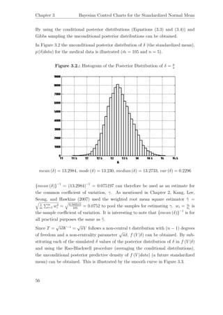
![3.4 Reference and Probability-Matching Priors for a Common Standardized Mean
The histogram in Figure 3.3 is obtained in the following way. Define a future sample
mean as ¯Xf and a future sample standard deviation as Sf . Since V =
¯Xf
Sf
=
˜Z
χ2
n−1
n−1
where ˜Z ∼ N δ, 1
n
, the histogram of the distribution of V is obtained by simulating
δ from the its posterior distribution and then ˜Z ∼ N δ, 1
n
. Simulate now a χ2
n−1
random variable and calculate V and repeat the process a large number of times. It
is clear that the two distributions are the same.
Figure 3.3.: Predictive Density f (V |data) for n = 5
mean (V ) = 16.6671, mode (V ) = 11.910, median (V ) = 14.276,
V ar (V ) = 75.0494
99.73% Equal-tail Interval = (6.212; 83.365)
99.73% HPD Interval = (5.176; 67.777)
According to this the 99.73% equal-tail interval for a future sample coefficient of
variation is (83.365)−1
; (6.212)−1
= [0.011995; 0.1609787]. For a 99.73% equal-tail
control chart for the coefficient of variation, Kang, Lee, Seong, and Hawkins (2007)
calculated the lower control limit as 0.1218, the upper control limit as 0.15957 and
as central line they used the root-mean square value ˆγ = 0.075. The frequentist
limits calculated by them are for all practical purposes the same as our Bayesian
57](https://image.slidesharecdn.com/328932de-d899-482b-a718-5e10677662e8-160621144849/85/thesis-65-320.jpg)


![Chapter 3 Bayesian Control Charts for the Standardized Normal Mean
3.5. Simulation Study
In this section a simulation study will be conducted to observe if the 95% Bayesian
confidence intervals for δ have the correct frequentist coverage.
For the simulation study the following combinations of parameters will be used:
µi 10 20 30 40 50 60 · · · 1000 1010 1020 · · · 1050
σi 0.75 1.5 2.25 3.0 3.75 · · · 75 · · · 78.15
which means that δ = µi
σi
= 13.3333, γ = 0.075, i = 1, 2, . . . , ¨m and ¨m = 105. These
parameter combinations are representative of the parameter values of the medical
dataset on patients undergoing organ transplantation analyzed by Kang, Lee, Seong,
and Hawkins (2007). As mentioned, the dataset consist of ¨m = 105 patients and
the number assays obtained for each patient is n = 5. As a common estimate for γ,
the weighted mean square ˆγ = 0.075 was used.
For the above given parameter combination a dataset can be simulated consisting of
¨m samples and n = 5 observations per sample. However since we are only interested
in the sufficient statistics ¯Xi and Si these can be simulated directly, namely ¯Xi ∼
N µi,
σ2
i
n
and S2
i ∼
σ2
i χ2
n−1
n−1
.
The simulated ¯Xi and S2
i (i = 1, 2, . . . , ¨m) values are then substituted in the con-
ditional posterior distributions given in Equation (3.3) and Equation (3.4). By
using the conditional posterior distributions and Gibbs sampling the unconditional
posterior distribution p (δ|data) can be obtained. A confidence interval for δ will
be calculated as follows: Simulate l = 10, 000 values of δ and sort the values in
ascending order ˜δ(1) ≤ ˜δ(2) ≤ · · · ≤ ˜δ(l).
Let K1 = α
2
l and K2 = 1 − α
2
l where [a] denotes the largest integer not greater
than a. ˜δ(K1), ˜δ(K2) is then a 100 (1 − α) % Bayesian confidence interval for δ. By
repeating the procedure for R = 3, 000 datasets it is found that the 3, 000, 95%
Bayesian confidence intervals (α = 0.05) cover the true parameter value δ = 13.333
in 2, 841 cases.
An estimate of the frequentist probability of coverage is therefore P ˜δ(K1) ≤ δ ≤ ˜δ(K2) =
0.9470. Also, P δ ≤ ˜δ(K1) = 0.0313 and P δ ≥ ˜δ(K2) = 0.0217.
For each dataset the posterior mean, δ∗
of the l = 10, 000 simulated δ values is
calculated as well as d = 13.3333 − δ∗
, the difference between the posterior mean
64](https://image.slidesharecdn.com/328932de-d899-482b-a718-5e10677662e8-160621144849/85/thesis-72-320.jpg)


![Chapter 4
Bayesian Control Charts for the Variance and Generalized Variance for the Normal
Distribution
obtained using the Rao-Blackwell method, i.e., the average of a large number of
unconditional run-lengths.
Figure 4.7.: Predictive Distribution of the “Run-length” f (r|data)for m = 10 and
n = 5 - Two-sided Control Chart
E (r|data) = 498.6473; Median (r|data) = 319; V ar (r|data) = 274473.1449
95% Equal − tail = [9; 1961]
In Figure 4.8 the distribution of the average run-length is given.
90](https://image.slidesharecdn.com/328932de-d899-482b-a718-5e10677662e8-160621144849/85/thesis-98-320.jpg)
![Mathematical Appendix
Figure 4.8.: Distribution of the Average “Run-length” - Two-sided Control Chart
Mean = 500; Median = 552; V ariance = 25572.95
95% Equal − tail = [92; 661]
Also the harmonic mean of the run-length is 1
β
. Therefore if β = 0.0027, the har-
monic mean is 1
0.0027
= 370.37 and if β = 0.0173, the harmonic mean is 1
0.0173
= 57.8
and the arithmetic mean is 370.
4.7. Conclusion
Phase I and Phase II control chart limits have been constructed using Bayesian
methodology. In this chapter we have seen that due to Monte Carlo simulation the
construction of control chart limits using the Bayesian paradigm are handled with
ease. Bayesian methods allow the use of any prior to construct control limits without
any difficulty. It has been shown that the uncertainty in unknown parameters are
handled with ease in using the predictive distribution in the determination of control
chart limits. It has also been shown that an increase in number of samples m and
the sample size n leads to a convergence in the run-length towards the expected
value of 370 at β = 0.0027.
91](https://image.slidesharecdn.com/328932de-d899-482b-a718-5e10677662e8-160621144849/85/thesis-99-320.jpg)


![Chapter 5 Tolerance Limits for Normal Populations
5.13. Conclusion
The first part of this chapter develops a Bayesian control chart for monitoring a
upper one-sided tolerance limit across a range of sample values. In the Bayesian
approach prior knowledge about the unknown parameters is formally incorporated
into the process of inference by assigning a prior distribution to the parameters.
The information contained in the prior is combined with the likelihood function to
obtain the posterior distribution. By using the posterior distribution the predictive
distribution of a upper one-sided tolerance limit can be obtained.
Determination of reasonable non-informative priors in multi-parameter problems is
not an easy task. The Jeffreys’ prior for example can have a bad effect on the pos-
terior distribution. Reference and probability matching priors are therefore derived
for the pth quantile of a normal distribution. The theory and results have been
applied to air-lead level data analyzed by Krishnamoorthy and Mathew (2009) to
illustrate the flexibility and unique features of the Bayesian simulation method for
obtaining posterior distributions, prediction intervals and run-lengths.
In the second part of this chapter the Bayesian procedure has been extended to
control charts of one-sided tolerance limits for a distribution of the difference between
two independent normal variables.
Mathematical Appendix to Chapter 5
Proof of Theorem 5.1
Assume Xi (i = 1, 2, . . . , n) are independently and identically Normally distributed
with mean µ and variance σ2
. The Fisher information matrix for the parameter
vector θ = [µ, σ2
] is given by
F µ, σ2
=
n
σ2 0
0 n
2(σ2)2
.
Let qp = µ + zpσ = t (µ, σ2
) = t (θ).
116](https://image.slidesharecdn.com/328932de-d899-482b-a718-5e10677662e8-160621144849/85/thesis-124-320.jpg)


![Mathematical Appendix
Now
f (ˆµf |µ, data) =
´ ∞
0
f (ˆµf |µ, θ) p (θ|µ, data) dθ
= m{n(¯x−µ)}n
Γ(n)
´ ∞
0
1
θ
n+2
exp −1
θ
[m (ˆµf − µ) + n (¯x − µ)] dθ
= nn+1(¯x−µ)n
m
[m(ˆµf −µ)+n(¯x−µ)]
n+1 ˆµf > 0
and
f (ˆµf |data) =
´ ˆµf
0
f (ˆµf , µ|data) dµ 0 < ˆµf < x(1)
=
´ x(1)
0
f (ˆµf , µ|data) dµ x(1) < ˆµf < ∞
where
f (ˆµf , µ|data) =
nn+1
(n − 1) m
1
ˆθ
n−1
− 1
¯x
n−1
{(mˆµf + n¯x) − µ (n + m)}−(n−1)
.
Therefore
f (ˆµf |data) = K∗ 1
n(¯x−ˆµf )
n
− 1
mˆµf +n¯x
n
0 < ˆµf < x(1)
= K∗ 1
m(ˆµf −x(1))+nˆθ
n
− 1
mˆµf +n¯x
n
x(1) < ˆµf < ∞
and
K∗
=
nn
(n − 1) m
(n + m)
1
ˆθ
n−1
−
1
¯x
n−1 −1
.
Proof of Theorem 6.7
Expected Value of ˆµf
141](https://image.slidesharecdn.com/328932de-d899-482b-a718-5e10677662e8-160621144849/85/thesis-149-320.jpg)


![Chapter 6 Two-Parameter Exponential Distribution
f ˆθf |data =
´ ∞
0
f ˆθf |θ p (θ|data) dθ
= mm−1
Γ(m−1)
ˆθf K1
´ ∞
0
1
θ
m+n−1
exp −1
θ
mˆθf + nˆθ − exp −1
θ
mˆθf + n¯x dθ
= mm−1
nn−1 Γ(m+n−2)
Γ(m−1)Γ(n−1)
1
ˆθ
n−1
− 1
¯x
n−1 −1
ˆθf
m−2
× 1
mˆθf +nˆθ
m+n−2
− 1
mˆθf +n¯x
m+n−2
ˆθf > 0.
Proof of Theorem 6.9
Expected Value of ˆθf
From Equation (6.1) it follows that
ˆθf |µ, θ ∼
χ2
2m−2
2m
θ.
Therefore
E ˆθf |µ, θ =
(m − 1)
m
θ
and
V ar ˆθf |µ, θ =
(m − 1)
m2
θ2
.
By using p (θ|µ, data) (given in Equation [6.5]) it follows that
E (θ|µ, data) =
n (¯x − µ)
(n − 1)
and therefore
E ˆθf |µ, data =
(m − 1)
m
n (¯x − µ)
(n − 1)
.
Since
p (µ|data) = ˜K (¯x − µ)−n
0 < µ < x(1)
146](https://image.slidesharecdn.com/328932de-d899-482b-a718-5e10677662e8-160621144849/85/thesis-154-320.jpg)


![7.6 Lower Control Limit for the Scale Parameter in Phase II
The distribution of Zmin obtained from 100,000 simulations is illustrated in Figure
7.3. The value Z0.05 = 0.0844 is calculated such that the FAP is at a level of 0.05.
The lower control limit is then determined as
LCL = Z0.05
m
i=1
ˆθi = (0.0844)(31.4701) = 2.656.
Since ˆθi > 2.656 (i = 1, 2, . . . , m∗
) it can be concluded that the scale parameter is
under statistical control.
7.6. Lower Control Limit for the Scale Parameter in
Phase II
In the first part of this section, the lower control limit in a Phase II setting will be
derived using the Bayesian predictive distribution.
The following theorems can easily be proved:
Theorem 7.7. For the two-parameter exponential distribution
f (xij; θ, µi) =
1
θ
exp −
1
θ
(xij − µi) i = 1, 2, . . . , m∗
, j = 1, 2, . . . , n, and xij > µi
the posterior distribution of the parameter θ given the data is given by
p (θ|data) =
nˆθ
m∗(n−1)
Γ [m∗ (n − 1)]
1
θ
m∗(n−1)+1
exp
−
nˆθ
θ
θ > 0
an Inverse Gamma Distribution.
Proof. The proof is given in the Mathematical Appendices to this chapter.
Theorem 7.8. Let ˆθf be the maximum likelihood estimator of the scale parameter
in a future sample of n observations, then the predictive distribution of ˆθf is
f ˆθf |data =
Γ [m∗
(n − 1) + n − 1]
Γ (n − 1) Γ [m∗ (n − 1)]
ˆθf
n−2
ˆθf + ˆθ
m∗(n−1)+n−1
ˆθf > 0
167](https://image.slidesharecdn.com/328932de-d899-482b-a718-5e10677662e8-160621144849/85/thesis-175-320.jpg)


![Chapter 7
Two-Parameter Exponential Distribution if the Location Parameter Can Take on
Any Value Between Minus Infinity and Plus Infinity
(b) The posterior distribution p (µ|data) is the same as the distribution of the pivotal
quantity Gµ = ˆµ −
χ2
2
χ2
2n−2
ˆθ.
Proof:
Let F =
χ2
2/2
χ2
2n−2/(2n−2)
∼ F2,2n−2
∴ g (f) = 1 + 1
n−1
f
−n
where 0 < f < ∞
We are interested in the distribution of µ = ˆµ − 2ˆθ
2n−2
F which means that F =
(n−1)
ˆθ
(ˆµ − µ) and dF
dµ
= (n−1)
ˆθ
.
Therefore
g (µ) = 1 + 1
ˆθ
(ˆµ − µ)
−n
n−1
ˆθ
= (n − 1) ˆθn−1 1
¯x−µ
n
where − ∞ < µ < ˆµ
= p (µ|data)
See Equation (7.5).
(c) The posterior distribution of p(µ|θ, data) is the same as the distribution of the
pivotal quantity Gµ|θ = ˆµ −
χ2
2
2n
θ (see Equation [7.1]).
Proof:
Let ˜Z ∼ χ2
2 then
g (˜z) = 1
2
exp −1
2
˜z .
Let µ = ˆµ − ˜z
2n
θ, then ˜z = 2n
θ
(ˆµ − µ) and d˜z
dµ
= 2n
θ
.
Therefore
g (µ|θ) = n
θ
exp −n
θ
(ˆµ − µ) −∞ < µ < ˆµ0
= p (µ|θ, data)
See Equation (6.4).
176](https://image.slidesharecdn.com/328932de-d899-482b-a718-5e10677662e8-160621144849/85/thesis-184-320.jpg)
![Mathematical Appendix
Proof of Theorem 7.2
As before
f (ˆµf |µ, θ) =
m
θ
exp −
m
θ
(ˆµf − µ) ˆµf > µ
and therefore
˜f (ˆµf |µ, data) =
ˆ ∞
0
f (ˆµf |µ, θ) ˜p (θ|µ, data) dθ.
Since
˜p (θ|µ, data) =
{n (¯x − µ)}n
Γ (n)
1
θ
n+1
exp −
n
θ
(¯x − µ)
it follows that
˜f (ˆµf |µ, data) =
nn+1
(¯x − µ)n
m
[m (ˆµf − µ) + n (¯x − µ)]n+1 ˆµf > µ.
For −∞ < µ < x(1),
˜p (µ|data) = (n − 1) ˆθ
n−1 1
¯x − µ
n
and
˜f (ˆµf , µ|data) = ˜f (ˆµf |µ, data) ˜p (µ|data)
=
nn+1m(n−1)(ˆθ)
n−1
[m(ˆµf −µ)+n(¯x−µ)]
n+1
.
Therefore
177](https://image.slidesharecdn.com/328932de-d899-482b-a718-5e10677662e8-160621144849/85/thesis-185-320.jpg)
![Chapter 7
Two-Parameter Exponential Distribution if the Location Parameter Can Take on
Any Value Between Minus Infinity and Plus Infinity
f (ˆµf |data) =
´ ˆµf
−∞
f (ˆµf , µ|data) dµ − ∞ < ˆµf < x(1)
=
´ x(1)
−∞
f (ˆµf , µ|data) dµ x(1) < ˆµf < ∞
= ˜K∗ 1
n(¯x−ˆµf )
n
− ∞ < ˆµf < x(1)
= ˜K∗ 1
nˆθ+m(ˆµf −x(1))
n
x(1) < ˆµf < ∞
where
˜K∗
=
nn
(n − 1) m
(n + m)
ˆθ
n−1
.
Proof of Theorem 7.4
From Equation (6.1) it follows that
ˆθf |θ ∼
χ2
2m−2
2m
θ
which means that
f ˆθf |θ =
m
θ
m−1 ˆθf
m−2
exp −m
θ
ˆθf
Γ (m − 1)
0 < ˆθf < ∞ (7.16)
The posterior distribution of θ (Equation [6.3]) is
˜p (θ|data) =
nˆθ
n−1
Γ (n − 1)
1
θ
n
exp −
n
θ
0 < θ < ∞.
Therefore
178](https://image.slidesharecdn.com/328932de-d899-482b-a718-5e10677662e8-160621144849/85/thesis-186-320.jpg)
![Mathematical Appendix
˜f ˆθf |data =
´ ∞
0
f ˆθf |θ ˜p (θ|data) dθ
= mm−1
Γ(m−1)
(nˆθ)
n−1
Γ(n−1)
ˆθf
m−2 ´ ∞
0
1
θ
m+n−1
exp −1
θ
mˆθf + nˆθ dθ
=
Γ(m+n−2)mm−1
(nˆθ)
n−1
(ˆθf )
m−2
Γ(m−1)Γ(n−1)(mˆθf +nˆθ)
m+n−2 0 < ˆθf < ∞.
Proof of Theorem 7.7
Let
ˆθ =
m∗
i=1
ˆθi.
As mentioned in Section 6 (see also Krishnamoorthy and Mathew (2009)) that it is
well known that
ˆθi ∼
θ
2n
χ2
2(n−1)
which means that
ˆθ ∼
θ
2n
χ2
2m∗(n−1).
Therefore
f ˆθ|θ =
n
θ
m∗(n−1) ˆθ
m∗(n−1)−1
exp −nˆθ
θ
Γ [m∗ (n − 1)]
= L θ|ˆθ
i.e, the likelihood function.
As before we will use as prior p (θ) ∝ θ−1
.
The posterior distribution
179](https://image.slidesharecdn.com/328932de-d899-482b-a718-5e10677662e8-160621144849/85/thesis-187-320.jpg)
![Chapter 7
Two-Parameter Exponential Distribution if the Location Parameter Can Take on
Any Value Between Minus Infinity and Plus Infinity
p θ|ˆθ = p (θ|data) ∝ L θ|ˆθ p (θ)
=
(nˆθ)
m∗(n−1)
Γ[m∗(n−1)]
1
θ
m∗(n−1)+1
exp −nˆθ
θ
An Inverse Gamma distribution.
Proof of Theorem 7.8
ˆθf |θ ∼
θ
2n
χ2
2(n−1).
Therefore
f ˆθf |data =
´ ∞
0
f ˆθf |θ p (θ|data) dθ
=
´ ∞
0
n
θ
n−1 (ˆθf )
n−2
exp −
nˆθf
θ
Γ(n−1)
×
(nˆθ)
m∗(n−1)
Γ[m∗(n−1)]
1
θ
m∗(n−1)+1
exp −nˆθ
θ
dθ
=
(n)n−1
(ˆθf )
n−2
(nˆθ)
m∗(n−1)
Γ(n−1)Γ[m∗(n−1)]
´ ∞
0
1
θ
m∗(n−1)+n
exp −n
θ
ˆθf + ˆθ dθ
=
Γ[m∗(n−1)+n−1](ˆθ)
m∗(n−1)
Γ(n−1)Γ[m∗(n−1)]
(ˆθf )
n−2
(ˆθf +ˆθ)
m∗(n−1)+n−1
ˆθf > 0
From this it follows that
ˆθf |data ∼
ˆθ
m∗
F2(n−1);2m∗(n−1)
where
ˆθ =
m∗
i=1
ˆθi.
180](https://image.slidesharecdn.com/328932de-d899-482b-a718-5e10677662e8-160621144849/85/thesis-188-320.jpg)


![Chapter 8 Piecewise Exponential Model
8.2. The Piecewise Exponential Model
The model in its simplest form can be written as
f (xj|µδ) =
δ
µ
jδ−1
−1
exp
−
xj
δ
µ
jδ−1
xj > 0.
The piecewise exponential model therefore assumes that the times between failures,
X1, X2, . . . , XJ are independent exponential random variables with
E (Xj) =
δ
µ
jδ−1
where δ > 0 and µ > 0.
For example if δ = 0.71 and µ = 0.0029, then the expected time between the 9th
and 10th failure is
E (X10) =
0.71
0.0029
100.71−1
= 125.56.
and the time between the 27th and 28th failure is
E (X28) =
0.71
0.0029
280.71−1
= 93.15.
In the PEXM model, µ is a scale parameter and δ is a shape parameter.
8.3. The Piecewise Exponential Model for Multiple
Repairable Systems
Using the same notation as in Arab et al. (2012), let xij denotes the time between
failures (j − 1) and j on system i for j = 1, 2, . . . , ni and i = 1, 2, . . . , k. The 0th
failure occurs at time 0. Also let N = k
i=1 ni denotes the total number of failures.
Finally let xi = [xi1,xi2, . . . , xi,ni
] denote the times between failures for the ith
system.
As in Arab et al. (2012) two cases for multiple systems will be considered.
184](https://image.slidesharecdn.com/328932de-d899-482b-a718-5e10677662e8-160621144849/85/thesis-192-320.jpg)


![Chapter 9 Process Capability Indices
then
p w|σ2
, y =
√
n
σ
√
2π
exp −
n
2
(w − ζ)2
σ2
+
n
σ
√
2π
exp −
n
2
(w + ζ)2
σ2
(See Kotz and Johnson (1993, page 26)).
Now C = b − ˜aw, where ˜a = 1
3σ
and b = Cp = u−l
6σ
.
Also w = − (C − b) 1
˜a
and dw
dc
= 1
˜a
.
From this it follows that
p C|σ2
, y =
√
n
˜aσ
√
2π
exp −
n
2˜a2σ2
[C − b + ˜aζ]2
+ exp −
n
2˜a2σ2
[C − b − ˜aζ]2
C < ˜b <
S
σ
where ˜b = ˆCp = u−l
6s
.
Substituting for ˜a, b and ζ and making use of the fact that k = vS2
σ2 ∼ χ2
v it follows
that
p C|k, y =
3
√
n
√
2π
exp
−
9n
2
C − t∗ k
v
2
+ exp
−
9n
2
C − ˜t
k
v
2
C < ˜b
k
v
.
Therefore
p C|y =
3
√
n
√
2π
ˆ ∞
C2v
˜b2
exp
−
9n
2
C − t∗ k
v
2
+ exp
−
9n
2
C − ˜t
k
v
2
×
1
2
v
2 Γ v
2
k
v
2
−1
exp −
k
2
dk.
246](https://image.slidesharecdn.com/328932de-d899-482b-a718-5e10677662e8-160621144849/85/thesis-254-320.jpg)


![A. MATLAB Code
A.1. MATLAB Code To Determine Coefficient of Variation from Sampling
Distribution
%Sampling distribution of cv for given R
clear
tic
R=0.0751;
n=5; f=n-1;
Fw=[];
h=0.001;
for w=0:h:0.2;
c=n./R./((n+f*(w.ˆ2)).ˆ0.5);
Aw=(fˆ(f/2))*sqrt(n)*abs(w.ˆ(f-1)).*exp(-n*f*(w.ˆ2)./2./(Rˆ2)
./(n+f*(w.ˆ2)))./(2ˆ((f-2)/2))/gamma(f/2)/sqrt(2*pi);
syms q
255](https://image.slidesharecdn.com/328932de-d899-482b-a718-5e10677662e8-160621144849/85/thesis-263-320.jpg)
![ChapterAMATLABCode
F=inline((q.ˆf).*exp((-((q-c).ˆ2))/2));
A=quad(F,10,30);
fw=Aw.*A./((n+f*(w.ˆ2)).ˆ((f+1)/2));
Fw=[Fw fw];
end
Fw=Fw/sum(Fw)/h;
w=0:h:0.2;
MEAN=w*Fw’/sum(Fw)
figure(1)
plot(w,Fw)
grid
CDF=cumsum(Fw)*h;
figure(2)
plot(w,CDF)
grid
toc
A.2. MATLAB Code to Simulate Coefficient of Variation from Berger Prior
clear
tic
X=[31.7 12.4
37.7 15.3
256](https://image.slidesharecdn.com/328932de-d899-482b-a718-5e10677662e8-160621144849/85/thesis-264-320.jpg)


![A.2MATLABCodetoSimulateCoefficientofVariationfromBergerPrior
769.5 9.7
772.7 9.6
791.6 2
799.9 11.4
948.6 5.2
971.8 11.1
991.2 8.8];
n=5;
Sig=X(:,1).*X(:,2)/100;
T=[]; SIG=[];
for k=1:2
lnD=0;
for j=1:length(X)
x=X(j,1);
s2=(x*X(j,2)/100).ˆ2;
D2=(n-1)*s2/n+xˆ2;
theta=0.02:0.00001:0.2;
lnA=-n*(1-xˆ2/D2)/2./(theta.ˆ2);
lnB=-(n*D2/2).*((1./Sig(j)-x./D2./theta).ˆ2);
lnd=lnA+lnB;
lnD=lnD+lnd;
end
261](https://image.slidesharecdn.com/328932de-d899-482b-a718-5e10677662e8-160621144849/85/thesis-269-320.jpg)
![ChapterAMATLABCode
lnC=-log(theta)-0.5*log(theta+0.5);
lnF=lnC+lnD;
M=max(lnF);
lnF=lnF-M;
ftheta=exp(lnF)/sum(exp(lnF));
%plot(theta,ftheta)
%grid
%pause
ct=cumsum(ftheta);
rt=rand(1,1);
t=theta(min(find(ct>=rt)));
T=[T;t];
s=1:0.001:200;
Sig=[];
for j=1:length(X)
x=X(j,1);
s2=(x*X(j,2)/100).ˆ2;
D2=(n-1)*s2/n+xˆ2;
lnfs=-(n+1)*log(s)-(n*D2/2).*((1./s-x./D2./t).ˆ2);
fsig=exp(lnfs)/sum(exp(lnfs));
%plot(s,fsig)
%grid
%pause
262](https://image.slidesharecdn.com/328932de-d899-482b-a718-5e10677662e8-160621144849/85/thesis-270-320.jpg)
![A.3MATLABCodetoDetermineSamplingandPredictiveDensitiesfor
CoefficientofVariation
cs=cumsum(fsig);
rc=rand(1,1);
sig=s(min(find(cs>=rc)));
Sig=[Sig;sig];
end
SIG=[SIG Sig];
end
toc
A.3. MATLAB Code to Determine Sampling and Predictive Densities for
Coefficient of Variation
%SAMPLING AND PREDICTIVE DISTRIBUTION OF CV
clear
tic
%load posterior_data
%load postcv5
%load simul_second
load postr1r2
FFw=[]; RR=[];
k=100;
for i=1:k
263](https://image.slidesharecdn.com/328932de-d899-482b-a718-5e10677662e8-160621144849/85/thesis-271-320.jpg)
![ChapterAMATLABCode
%i
R=R2(round(rand*length(R2)));
%R=0.0977; %51;
n=5; f=n-1;
Fw=[];
for w=0:0.001:0.25;
c=n./R./((n+f*(w.ˆ2)).ˆ0.5);
Aw=(fˆ(f/2))*sqrt(n)*abs(w.ˆ(f-1)).*exp(-n*f*(w.ˆ2)./2./(Rˆ2)
./(n+f*(w.ˆ2)))./(2ˆ((f-2)/2))/gamma(f/2)/sqrt(2*pi);
h=0.002;
q=15:h:40;
F=(q.ˆf).*exp((-((q-c).ˆ2))/2);
If=h*sum(F);
%plot(q,F)
%grid
%pause
fw=Aw.*If./((n+f*(w.ˆ2)).ˆ((f+1)/2));
Fw=[Fw fw];
end
FFw=[FFw;Fw];
RR=[RR;R];
end
w=0:0.001:0.25;
MFw=mean(FFw);
264](https://image.slidesharecdn.com/328932de-d899-482b-a718-5e10677662e8-160621144849/85/thesis-272-320.jpg)


![ChapterAMATLABCode
%Determine the test value to determine rejection region for Chi2 with v
%degrees of freedom;
critval = (1/m).*simval.*Fval;
critval2 = (1/m).*simval.*Fval2;
%Determine rejection region;
rejreg = 1-chi2cdf(critval,v)+chi2cdf(critval2,v);
q = 1-rejreg;
meanrl = mean(q./rejreg);
meanrl1 = mean(1./rejreg);
medianrl = median(q./rejreg);
medianrl1 = median(1./rejreg);
stdrl = std(q./rejreg);
stdrl1 = std(1./rejreg);
rl = sort(q./rejreg);
rllow = rl(0.025*nsim);
rlhigh = rl(0.975*nsim);
disp(meanrl)
disp(medianrl)
disp([rllow rlhigh])
268](https://image.slidesharecdn.com/328932de-d899-482b-a718-5e10677662e8-160621144849/85/thesis-276-320.jpg)

![ChapterAMATLABCode
A.6. MATLAB Code to Determine Rejection Region for the Generalized
Variance
function [meanrl,medianrl,rllow,rlhigh,rl] = varrlmp(n,m,p,alpha)
%Initial Values;
nsim = 30000;
rejregsim = 1000000;
%Vector of p’s;
vecp = 1:p;
%F-values;
Fconst = ((n-vecp)./(m*(n-1)+1-vecp));
Fs = zeros(p,rejregsim);
for k = vecp
Fs(k,:) = frnd((n-k),(m*(n-1)+1-k),1,rejregsim);
end
if p ˜= 1
Fcomb = prod(Fs);
else
Fcomb = Fs;
end
270](https://image.slidesharecdn.com/328932de-d899-482b-a718-5e10677662e8-160621144849/85/thesis-278-320.jpg)


![A.7MATLABCodetoDetermineRejectionRegionofToleranceInterval
%data;
data.orig = [200 120 15 7 8 6 48 61 380 80 29 1000 350 1400 110];
%take the logarithm of the data;
data.log = log(data.orig);
%determine the mean and sample standard deviation of log data;
data.logmean = mean(data.log);
data.var = var(data.log);
data.sd = std(data.log);
%determine k1 from the non-central t distribution;
data.size = size(data.orig);
df = data.size(2) - 1;
ncparam = norminv(0.95,0,1)*sqrt(data.size(2));
k1 = nctinv((1-alpha),df,ncparam)/sqrt(data.size(2));
%Upper tolerance limit;
data.utl = data.logmean + k1*data.sd;
%Simulate future values;
nsim = 10000;
x = 1:0.1:16;
273](https://image.slidesharecdn.com/328932de-d899-482b-a718-5e10677662e8-160621144849/85/thesis-281-320.jpg)


![A.8MATLABCodetoDetermineRejectionRegionofµfromtheTwoParameter
ExponentialDistribution
paralph = n;
parlam = n.*(xbar-musim);
thsim = 1./gamrnd(paralph,1./parlam);
% musim = [149.3 146.1 135.2 102.25 152.9];
% thsim = [856.6 618.0 1047.2 1054.1 704.4];
%Determine psi;
rlprob = zeros(1,nsim);
for k = 1:nsim
parm = thsim(k)/m;
c = max(LCL,musim(k));
rlprob(k) = 1 - exp(m*musim(k)/thsim(k))*(expcdf(UCL,parm)-expcdf(c,parm));
end
rl = (1-rlprob)./rlprob;
rlplot = rl(rl<2500);
hist(rlplot,50),xlabel(’E(r|mu,theta)’,’fontsize’,16);
h = findobj(gca,’Type’,’patch’);
set(h,’FaceColor’,’w’,’EdgeColor’,’k’);
set(gca,’fontsize’,14);
save(’murl.mat’)
277](https://image.slidesharecdn.com/328932de-d899-482b-a718-5e10677662e8-160621144849/85/thesis-285-320.jpg)


![A.17MATLABCodeforGaneshSimulation
hist(rl.rltwo,50),xlabel(’$E(r|mu,sigmaˆ2)$’,’fontsize’,20);
h = findobj(gca,’Type’,’patch’);
set(h,’FaceColor’,’w’,’EdgeColor’,’k’);
set(gca,’fontsize’,14);
%save(’rlres.mat’);
A.17. MATLAB Code for Ganesh Simulation
clear
tic
n=[50;75;70;75];
x=[2.7048;2.7019;2.6979;2.6972];
s=[0.0034;0.0055;0.0046;0.0038];
%n=n(3); x=x(3); s=s(3);
LSL=2.6795; USL=2.7205;
k=4;
%Cphat=(USL-LSL)./6./s;
%Cpuhat=(USL-x)./3./s;
%Cplhat=(x-LSL)./3./s;
%Cpl=[]; Cpu=[];
Cpk=[];
N=100000;
299](https://image.slidesharecdn.com/328932de-d899-482b-a718-5e10677662e8-160621144849/85/thesis-307-320.jpg)
![ChapterAMATLABCode
for i=1:N
sig=s.*sqrt((n-1)./chi2rnd(n-1));
cpl=normrnd((x-LSL)./3./sig,1./3./sqrt(n));
cpu=normrnd((USL-x)./3./sig,1./3./sqrt(n));
%Cpl=[Cpl;cpl’];
%Cpu=[Cpu;cpu’];
cpk=min([cpl’;cpu’]);
Cpk=[Cpk;cpk];
end
M=mean(Cpk);
A=Cpk-ones(N,1)*M;
T2=[];
for j=1:N
t2=max(A(j,:))-min(A(j,:));
T2=[T2;t2];
end
toc
hist(T2,50);
set(0, ’defaultTextInterpreter’, ’latex’);
h = findobj(gca,’Type’,’patch’), xlabel(’$Tˆ{(2)}$’,’fontsize’,20);
set(h,’FaceColor’,’w’,’EdgeColor’,’k’);
set(gca,’fontsize’,14);
300](https://image.slidesharecdn.com/328932de-d899-482b-a718-5e10677662e8-160621144849/85/thesis-308-320.jpg)