Downloaded 4,552 times

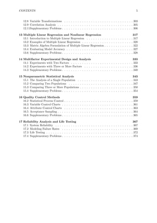

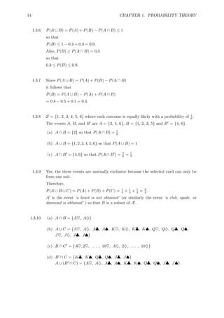
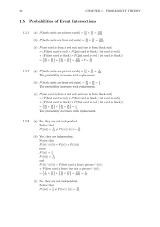
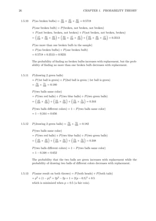
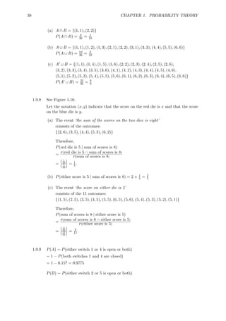

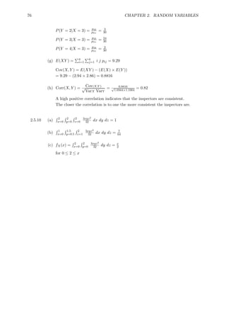
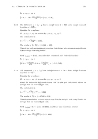
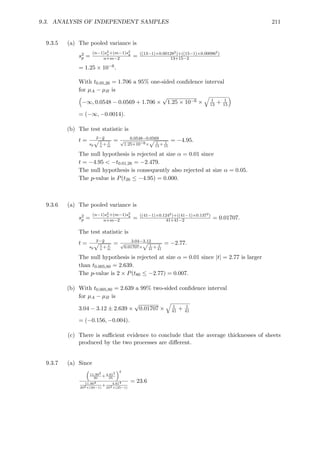
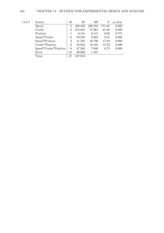
![54 CHAPTER 2. RANDOM VARIABLES
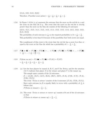
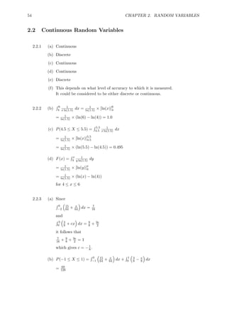
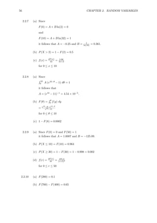
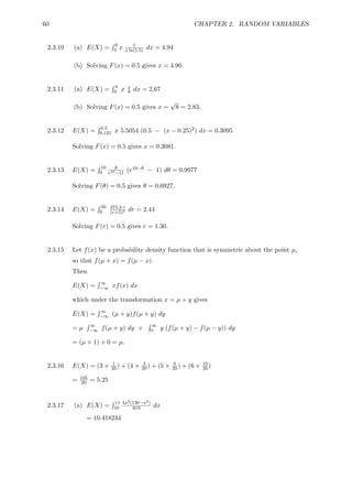
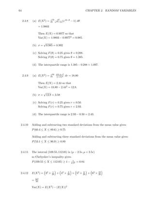
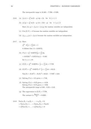
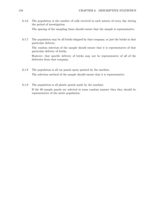
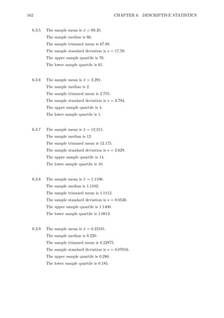
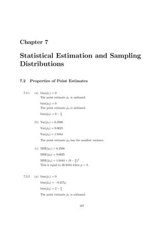
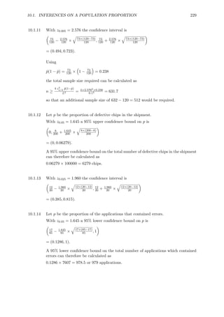
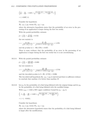
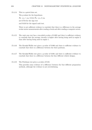
2.2 Continuous Random Variables
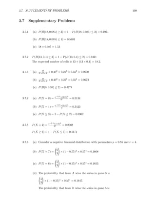
2.2.1 (a) Continuous
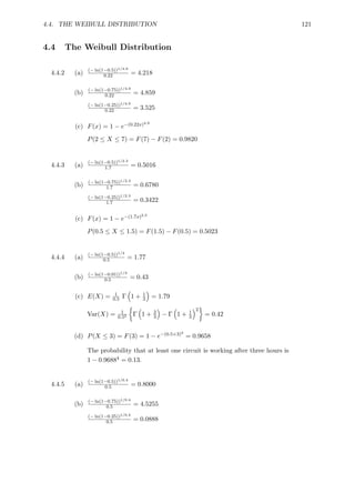
(b) Discrete
(c) Continuous
(d) Continuous
(e) Discrete
(f) This depends on what level of accuracy to which it is measured.
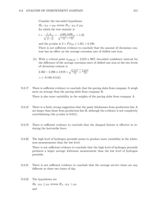
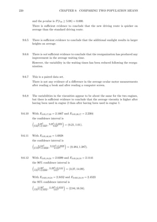
It could be considered to be either discrete or continuous.
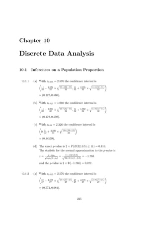
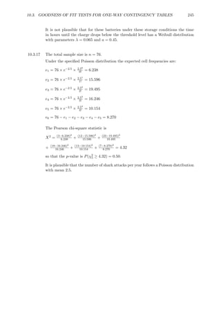
2.2.2 (b)
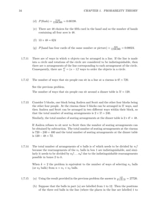
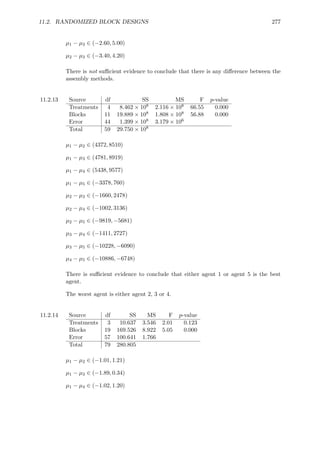
R 6
4
1
dx = 1
× [ln(x)]6
x ln(1.5) ln(1.5) 4
ln(1.5) × (ln(6) − ln(4)) = 1.0
= 1
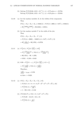
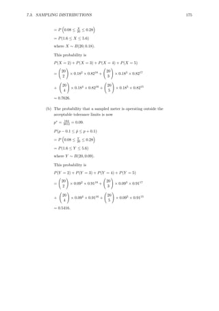
(c) P(4.5 X 5.5) =
R 5.5
4.5
1
x ln(1.5) dx
ln(1.5) × [ln(x)]5.5
= 1
4.5
= 1
ln(1.5) × (ln(5.5) − ln(4.5)) = 0.495
(d) F(x) =
R x
4
1
y ln(1.5) dy
ln(1.5) × [ln(y)]x
= 1
4
= 1
× (ln(x) − ln(4))
ln(1.5) for 4 x 6
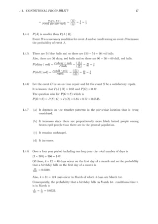
2.2.3 (a) Since
R 0
−2
15
64 + x
64
dx = 7
16
and
R 3
0
3
8 + cx
dx = 9
8 + 9c
2
it follows that
7
16 + 9
8 + 9c
2 = 1
which gives c = −1
8 .
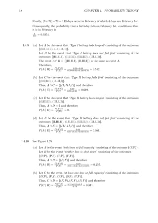
(b) P(−1 X 1) =
R 0
−1
15
64 + x
64
dx +
R 1
0
3
8 − x
8
dx
= 69
128](https://image.slidesharecdn.com/prosol3rd-141006212339-conversion-gate01/85/Manual-Solution-Probability-and-Statistic-Hayter-4th-Edition-56-320.jpg)
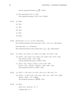

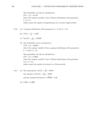


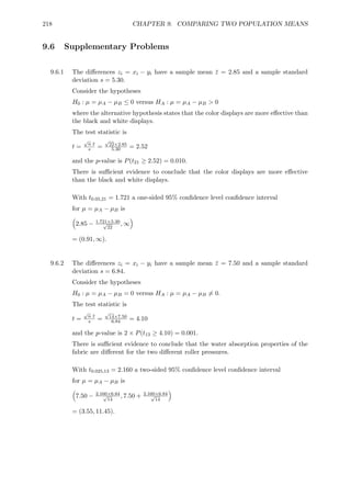


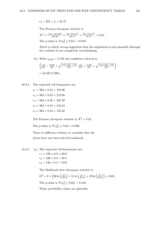
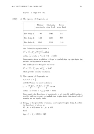
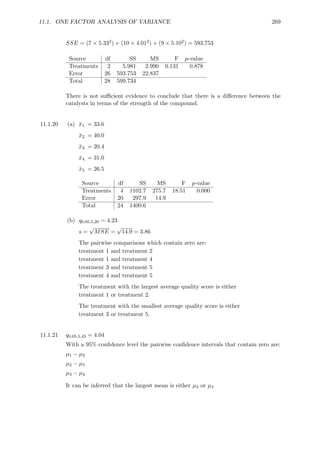

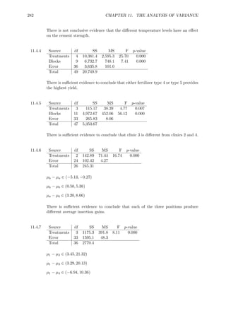

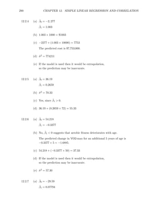


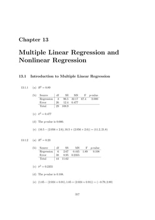
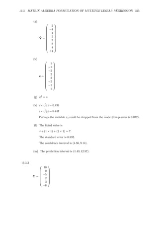


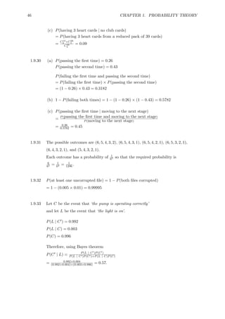
The instructor solution manual for 'Probability and Statistics for Engineers and Scientists' by Anthony Hayter includes detailed solutions and answers to all problems, complementing the student manual which only covers odd-numbered problems. The manual spans various topics in probability theory, random variables, probability distributions, statistics, and nonparametric analysis, providing a comprehensive guide for instructors. It is structured to enhance teaching and understanding of the material covered in the textbook.