Introductory Statistics Explained.pdf

.
Introductory Statistics Explained
Edition 1.10CC
©2015 Jeremy Balka
This work is licensed under:
https://creativecommons.org/licenses/by-nc-nd/4.0/
See http://www.jbstatistics.com/ for the complete set of supporting videos
and other supporting material.
The complete set of videos is also available at:
https://www.youtube.com/user/jbstatistics/videos

Contents
1 Introduction 1
1.1 Introduction . . . . . . . . . . . . . . . . . . . . . . . . . . . . . . 2
1.2 Descriptive Statistics . . . . . . . . . . . . . . . . . . . . . . . . . 2
1.3 Inferential Statistics . . . . . . . . . . . . . . . . . . . . . . . . . 3
2 Gathering Data 7
2.1 Introduction . . . . . . . . . . . . . . . . . . . . . . . . . . . . . . 9
2.2 Populations and Samples, Parameters and Statistics . . . . . . . 9
2.3 Types of Sampling . . . . . . . . . . . . . . . . . . . . . . . . . . 10
2.3.1 Simple Random Sampling . . . . . . . . . . . . . . . . . . 11
2.3.2 Other Types of Random Sampling . . . . . . . . . . . . . 13
2.4 Experiments and Observational Studies . . . . . . . . . . . . . . 14
2.5 Chapter Summary . . . . . . . . . . . . . . . . . . . . . . . . . . 19
3 Descriptive Statistics 21
3.1 Introduction . . . . . . . . . . . . . . . . . . . . . . . . . . . . . . 23
3.2 Plots for Categorical and Quantitative Variables . . . . . . . . . 23
3.2.1 Plots for Categorical Variables . . . . . . . . . . . . . . . 23
3.2.2 Graphs for Quantitative Variables . . . . . . . . . . . . . 25
3.3 Numerical Measures . . . . . . . . . . . . . . . . . . . . . . . . . 32
3.3.1 Summation Notation . . . . . . . . . . . . . . . . . . . . . 33
3.3.2 Measures of Central Tendency . . . . . . . . . . . . . . . . 34
3.3.3 Measures of Variability . . . . . . . . . . . . . . . . . . . . 37
3.3.4 Measures of Relative Standing . . . . . . . . . . . . . . . 45
3.4 Boxplots . . . . . . . . . . . . . . . . . . . . . . . . . . . . . . . . 50
3.5 Linear Transformations . . . . . . . . . . . . . . . . . . . . . . . . 53
3.6 Chapter Summary . . . . . . . . . . . . . . . . . . . . . . . . . . 56
4 Probability 59
4.1 Introduction . . . . . . . . . . . . . . . . . . . . . . . . . . . . . . 61
4.2 Basics of Probability . . . . . . . . . . . . . . . . . . . . . . . . . 62
4.2.1 Interpreting Probability . . . . . . . . . . . . . . . . . . . 62
i

Balka ISE 1.10 CONTENTS ii
4.2.2 Sample Spaces and Sample Points . . . . . . . . . . . . . 63
4.2.3 Events . . . . . . . . . . . . . . . . . . . . . . . . . . . . . 64
4.3 Rules of Probability . . . . . . . . . . . . . . . . . . . . . . . . . 65
4.3.1 The Intersection of Events . . . . . . . . . . . . . . . . . . 65
4.3.2 Mutually Exclusive Events . . . . . . . . . . . . . . . . . . 65
4.3.3 The Union of Events and the Addition Rule . . . . . . . . 66
4.3.4 Complementary Events . . . . . . . . . . . . . . . . . . . 67
4.3.5 An Example . . . . . . . . . . . . . . . . . . . . . . . . . . 67
4.3.6 Conditional Probability . . . . . . . . . . . . . . . . . . . 69
4.3.7 Independent Events . . . . . . . . . . . . . . . . . . . . . 71
4.3.8 The Multiplication Rule . . . . . . . . . . . . . . . . . . . 73
4.4 Examples . . . . . . . . . . . . . . . . . . . . . . . . . . . . . . . 75
4.5 Bayes’ Theorem . . . . . . . . . . . . . . . . . . . . . . . . . . . . 82
4.5.1 Introduction . . . . . . . . . . . . . . . . . . . . . . . . . . 82
4.5.2 The Law of Total Probability and Bayes’ Theorem . . . . 85
4.6 Counting rules: Permutations and Combinations . . . . . . . . . 88
4.6.1 Permutations . . . . . . . . . . . . . . . . . . . . . . . . . 89
4.6.2 Combinations . . . . . . . . . . . . . . . . . . . . . . . . . 90
4.7 Probability and the Long Run . . . . . . . . . . . . . . . . . . . . 91
4.8 Chapter Summary . . . . . . . . . . . . . . . . . . . . . . . . . . 94
5 Discrete Random Variables and Discrete Probability Distribu-
tions 97
5.1 Introduction . . . . . . . . . . . . . . . . . . . . . . . . . . . . . . 99
5.2 Discrete and Continuous Random Variables . . . . . . . . . . . . 99
5.3 Discrete Probability Distributions . . . . . . . . . . . . . . . . . . 101
5.3.1 The Expectation and Variance of Discrete Random Variables102
5.4 The Bernoulli Distribution . . . . . . . . . . . . . . . . . . . . . . 110
5.5 The Binomial Distribution . . . . . . . . . . . . . . . . . . . . . . 111
5.5.1 Binomial or Not? . . . . . . . . . . . . . . . . . . . . . . . 114
5.5.2 A Binomial Example with Probability Calculations . . . . 115
5.6 The Hypergeometric Distribution . . . . . . . . . . . . . . . . . . 117
5.7 The Poisson Distribution . . . . . . . . . . . . . . . . . . . . . . . 121
5.7.1 Introduction . . . . . . . . . . . . . . . . . . . . . . . . . . 121
5.7.2 The Relationship Between the Poisson and Binomial Dis-
tributions . . . . . . . . . . . . . . . . . . . . . . . . . . . 123
5.7.3 Poisson or Not? More Discussion on When a Random Vari-
able has a Poisson distribution . . . . . . . . . . . . . . . 125
5.8 The Geometric Distribution . . . . . . . . . . . . . . . . . . . . . 127
5.9 The Negative Binomial Distribution . . . . . . . . . . . . . . . . 131
5.10 The Multinomial Distribution . . . . . . . . . . . . . . . . . . . . 133
5.11 Chapter Summary . . . . . . . . . . . . . . . . . . . . . . . . . . 135

Balka ISE 1.10 CONTENTS iii
6 Continuous Random Variables and Continuous Probability Dis-
tributions 139
6.1 Introduction . . . . . . . . . . . . . . . . . . . . . . . . . . . . . . 141
6.2 Properties of Continuous Probability Distributions . . . . . . . . 143
6.2.1 An Example Using Integration . . . . . . . . . . . . . . . 144
6.3 The Continuous Uniform Distribution . . . . . . . . . . . . . . . 146
6.4 The Normal Distribution . . . . . . . . . . . . . . . . . . . . . . . 150
6.4.1 Finding Areas Under the Standard Normal Curve . . . . . 153
6.4.2 Standardizing Normally Distributed Random Variables . . 158
6.5 Normal Quantile-Quantile Plots . . . . . . . . . . . . . . . . . . . 162
6.5.1 Examples of Normal QQ Plots . . . . . . . . . . . . . . . 163
6.6 Other Important Continuous Probability Distributions . . . . . . 166
6.6.1 The χ2 Distribution . . . . . . . . . . . . . . . . . . . . . 166
6.6.2 The t Distribution . . . . . . . . . . . . . . . . . . . . . . 168
6.6.3 The F Distribution . . . . . . . . . . . . . . . . . . . . . . 169
6.7 Chapter Summary . . . . . . . . . . . . . . . . . . . . . . . . . . 172
7 Sampling Distributions 175
7.1 Introduction . . . . . . . . . . . . . . . . . . . . . . . . . . . . . . 177
7.2 The Sampling Distribution of the Sample Mean . . . . . . . . . . 180
7.3 The Central Limit Theorem . . . . . . . . . . . . . . . . . . . . . 183
7.3.1 Illustration of the Central Limit Theorem . . . . . . . . . 185
7.4 Some Terminology Regarding Sampling Distributions . . . . . . . 187
7.4.1 Standard Errors . . . . . . . . . . . . . . . . . . . . . . . 187
7.4.2 Unbiased Estimators . . . . . . . . . . . . . . . . . . . . . 187
7.5 Chapter Summary . . . . . . . . . . . . . . . . . . . . . . . . . . 188
8 Confidence Intervals 191
8.1 Introduction . . . . . . . . . . . . . . . . . . . . . . . . . . . . . . 193
8.2 Interval Estimation of µ when σ is Known . . . . . . . . . . . . . 194
8.2.1 Interpretation of the Interval . . . . . . . . . . . . . . . . 198
8.2.2 What Factors Affect the Margin of Error? . . . . . . . . . 200
8.2.3 Examples . . . . . . . . . . . . . . . . . . . . . . . . . . . 202
8.3 Confidence Intervals for µ When σ is Unknown . . . . . . . . . . 205
8.3.1 Introduction . . . . . . . . . . . . . . . . . . . . . . . . . . 205
8.3.2 Examples . . . . . . . . . . . . . . . . . . . . . . . . . . . 208
8.3.3 Assumptions of the One-Sample t Procedures . . . . . . . 212
8.4 Determining the Minimum Sample Size n . . . . . . . . . . . . . 218
8.5 Chapter Summary . . . . . . . . . . . . . . . . . . . . . . . . . . 220
9 Hypothesis Tests (Tests of Significance) 223
9.1 Introduction . . . . . . . . . . . . . . . . . . . . . . . . . . . . . . 225
9.2 The Logic of Hypothesis Testing . . . . . . . . . . . . . . . . . . 227

Balka ISE 1.10 CONTENTS iv
9.3 Hypothesis Tests for µ When σ is Known . . . . . . . . . . . . . 229
9.3.1 Constructing Appropriate Hypotheses . . . . . . . . . . . 229
9.3.2 The Test Statistic . . . . . . . . . . . . . . . . . . . . . . 230
9.3.3 The Rejection Region Approach to Hypothesis Testing . . 233
9.3.4 P-values . . . . . . . . . . . . . . . . . . . . . . . . . . . . 235
9.4 Examples . . . . . . . . . . . . . . . . . . . . . . . . . . . . . . . 239
9.5 Interpreting the p-value . . . . . . . . . . . . . . . . . . . . . . . 243
9.5.1 The Distribution of the p-value When H0 is True . . . . . 243
9.5.2 The Distribution of the p-value When H0 is False . . . . . 245
9.6 Type I Errors, Type II Errors, and the Power of a Test . . . . . . 245
9.6.1 Calculating Power and the Probability of a Type II Error 248
9.6.2 What Factors Affect the Power of the Test? . . . . . . . . 253
9.7 One-sided Test or Two-sided Test? . . . . . . . . . . . . . . . . . 254
9.7.1 Choosing Between a One-sided Alternative and a Two-
sided Alternative . . . . . . . . . . . . . . . . . . . . . . . 254
9.7.2 Reaching a Directional Conclusion from a Two-sided Al-
ternative . . . . . . . . . . . . . . . . . . . . . . . . . . . . 256
9.8 Statistical Significance and Practical Significance . . . . . . . . . 257
9.9 The Relationship Between Hypothesis Tests and
Confidence Intervals . . . . . . . . . . . . . . . . . . . . . . . . . 258
9.10 Hypothesis Tests for µ When σ is Unknown . . . . . . . . . . . . 260
9.10.1 Examples of Hypothesis Tests Using the t Statistic . . . . 261
9.11 More on Assumptions . . . . . . . . . . . . . . . . . . . . . . . . 266
9.12 Criticisms of Hypothesis Testing . . . . . . . . . . . . . . . . . . 268
9.13 Chapter Summary . . . . . . . . . . . . . . . . . . . . . . . . . . 271
10 Inference for Two Means 273
10.1 Introduction . . . . . . . . . . . . . . . . . . . . . . . . . . . . . . 275
10.2 The Sampling Distribution of the Difference in Sample Means . . 276
10.3 Inference for µ1 − µ2 When σ1 and σ2 are Known . . . . . . . . . 277
10.4 Inference for µ1 − µ2 when σ1 and σ2 are unknown . . . . . . . . 279
10.4.1 Pooled Variance Two-Sample t Procedures . . . . . . . . . 280
10.4.2 The Welch Approximate t Procedure . . . . . . . . . . . . 286
10.4.3 Guidelines for Choosing the Appropriate Two-Sample
t Procedure . . . . . . . . . . . . . . . . . . . . . . . . . . 290
10.4.4 More Examples of Inferences for the Difference in Means . 292
10.5 Paired-Difference Procedures . . . . . . . . . . . . . . . . . . . . 297
10.5.1 The Paired-Difference t Procedure . . . . . . . . . . . . . 300
10.6 Pooled-Variance t Procedures: Investigating the Normality As-
sumption . . . . . . . . . . . . . . . . . . . . . . . . . . . . . . . 303
10.7 Chapter Summary . . . . . . . . . . . . . . . . . . . . . . . . . . 306
11 Inference for Proportions 309

Balka ISE 1.10 CONTENTS v
11.1 Introduction . . . . . . . . . . . . . . . . . . . . . . . . . . . . . . 311
11.2 The Sampling Distribution of the Sample Proportion . . . . . . . 312
11.2.1 The Mean and Variance of the Sampling Distribution of p̂ 312
11.2.2 The Normal Approximation . . . . . . . . . . . . . . . . . 313
11.3 Confidence Intervals and Hypothesis Tests for the Population Pro-
portion p . . . . . . . . . . . . . . . . . . . . . . . . . . . . . . . 314
11.3.1 Examples . . . . . . . . . . . . . . . . . . . . . . . . . . . 316
11.4 Determining the Minimum Sample Size n . . . . . . . . . . . . . 320
11.5 Inference Procedures for Two Population Proportions . . . . . . . 321
11.5.1 The Sampling Distribution of p̂1 − p̂2 . . . . . . . . . . . . 322
11.5.2 Confidence Intervals and Hypothesis Tests for p1 − p2 . . 323
11.6 More on Assumptions . . . . . . . . . . . . . . . . . . . . . . . . 327
11.7 Chapter Summary . . . . . . . . . . . . . . . . . . . . . . . . . . 329
12 Inference for Variances 331
12.1 Introduction . . . . . . . . . . . . . . . . . . . . . . . . . . . . . . 333
12.2 The Sampling Distribution of the Sample Variance . . . . . . . . 334
12.2.1 The Sampling Distribution of the Sample Variance When
Sampling from a Normal Population . . . . . . . . . . . . 334
Sampling from Non-Normal Populations . . . . . . . . . . 336
12.3 Inference Procedures for a Single Variance . . . . . . . . . . . . . 337
12.4 Comparing Two Variances . . . . . . . . . . . . . . . . . . . . . . 343
12.4.1 The Sampling Distribution of the Ratio of Sample Variances343
12.4.2 Inference Procedures for the Ratio of Population Variances 345
12.5 Investigating the Effect of Violations of the Normality Assumption 352
12.5.1 Inference Procedures for One Variance: How Robust are
these Procedures? . . . . . . . . . . . . . . . . . . . . . . 352
12.5.2 Inference Procedures for the Ratio of Variances: How Ro-
bust are these Procedures? . . . . . . . . . . . . . . . . . 355
12.6 Chapter Summary . . . . . . . . . . . . . . . . . . . . . . . . . . 357
13 χ2 Tests for Count Data 359
13.1 Introduction . . . . . . . . . . . . . . . . . . . . . . . . . . . . . . 361
13.2 χ2 Tests for One-Way Tables . . . . . . . . . . . . . . . . . . . . 361
13.2.1 The χ2 Test Statistic . . . . . . . . . . . . . . . . . . . . . 362
13.2.2 Testing Goodness-of-Fit for Specific Parametric Distributions366
13.3 χ2 Tests for Two-Way Tables . . . . . . . . . . . . . . . . . . . . 368
13.3.1 The χ2 Test Statistic for Two-Way Tables . . . . . . . . . 370
13.3.2 Examples . . . . . . . . . . . . . . . . . . . . . . . . . . . 371
13.4 A Few More Points . . . . . . . . . . . . . . . . . . . . . . . . . . 375
13.4.1 Relationship Between the Z Test and χ2 Test for 2×2 Tables375
13.4.2 Assumptions . . . . . . . . . . . . . . . . . . . . . . . . . 376

Balka ISE 1.10 CONTENTS vi
13.5 Chapter Summary . . . . . . . . . . . . . . . . . . . . . . . . . . 379
14 One-Way Analysis of Variance (ANOVA) 381
14.1 Introduction . . . . . . . . . . . . . . . . . . . . . . . . . . . . . . 383
14.2 One-Way ANOVA . . . . . . . . . . . . . . . . . . . . . . . . . . 384
14.3 Carrying Out the One-Way Analysis of Variance . . . . . . . . . 386
14.3.1 The Formulas . . . . . . . . . . . . . . . . . . . . . . . . . 386
14.3.2 An Example with Full Calculations . . . . . . . . . . . . . 388
14.4 What Should be Done After One-Way ANOVA? . . . . . . . . . 391
14.4.1 Introduction . . . . . . . . . . . . . . . . . . . . . . . . . . 391
14.4.2 Fisher’s LSD Method . . . . . . . . . . . . . . . . . . . . . 393
14.4.3 The Bonferroni Correction . . . . . . . . . . . . . . . . . . 395
14.4.4 Tukey’s Honest Significant Difference Method . . . . . . . 398
14.5 Examples . . . . . . . . . . . . . . . . . . . . . . . . . . . . . . . 401
14.6 A Few More Points . . . . . . . . . . . . . . . . . . . . . . . . . . 406
14.6.1 Different Types of Experimental Design . . . . . . . . . . 406
14.6.2 One-Way ANOVA and the Pooled-Variance t Test . . . . 407
14.6.3 ANOVA Assumptions . . . . . . . . . . . . . . . . . . . . 407
14.7 Chapter Summary . . . . . . . . . . . . . . . . . . . . . . . . . . 408
15 Introduction to Simple Linear Regression 411
15.1 Introduction . . . . . . . . . . . . . . . . . . . . . . . . . . . . . . 413
15.2 The Linear Regression Model . . . . . . . . . . . . . . . . . . . . 413
15.3 The Least Squares Regression Line . . . . . . . . . . . . . . . . . 417
15.4 Statistical Inference in Simple Linear Regression . . . . . . . . . 420
15.4.1 Model Assumptions . . . . . . . . . . . . . . . . . . . . . 421
15.4.2 Statistical Inference for the Parameter β1 . . . . . . . . . 422
15.5 Checking Model Assumptions with Residual Plots . . . . . . . . . 424
15.6 Measures of the Strength of the Linear Relationship . . . . . . . 426
15.6.1 The Pearson Correlation Coefficient . . . . . . . . . . . . 426
15.6.2 The Coefficient of Determination . . . . . . . . . . . . . . 429
15.7 Estimation and Prediction Using the Fitted Line . . . . . . . . . 431
15.8 Transformations . . . . . . . . . . . . . . . . . . . . . . . . . . . . 433
15.9 A Complete Example . . . . . . . . . . . . . . . . . . . . . . . . . 435
15.10Outliers, Leverage, and Influential Points . . . . . . . . . . . . . . 437
15.11Some Cautions about Regression and Correlation . . . . . . . . . 439
15.11.1Always Plot Your Data . . . . . . . . . . . . . . . . . . . 439
15.11.2Avoid Extrapolating . . . . . . . . . . . . . . . . . . . . . 440
15.11.3Correlation Does Not Imply Causation . . . . . . . . . . . 441
15.12A Brief Multiple Regression Example . . . . . . . . . . . . . . . . 442
15.13Chapter Summary . . . . . . . . . . . . . . . . . . . . . . . . . . 446

Chapter 1
Introduction
“I have been impressed with the urgency of doing. Knowing is not enough; we
must apply. Being willing is not enough; we must do.”
-Leonardo da Vinci
1

Balka ISE 1.10 1.1. INTRODUCTION 2
1.1 Introduction
When first encountering the study of statistics, students often have a preconceived—
and incorrect—notion of what the field of statistics is all about. Some people
think that statisticians are able to quote all sorts of unusual statistics, such as
32% of undergraduate students report patterns of harmful drinking behaviour,
or that 55% of undergraduates do not understand what the field of statistics is
all about. But the field of statistics has little to do with quoting obscure percent-
ages or other numerical summaries. In statistics, we often use data to answer
questions like:
• Is a newly developed drug more effective than one currently in use?
• Is there a still a sex effect in salaries? After accounting for other relevant
variables, is there a difference in salaries between men and women? Can
we estimate the size of this effect for different occupations?
• Can post-menopausal women lower their heart attack risk by undergoing
hormone replacement therapy?
To answer these types of questions, we will first need to find or collect appropriate
data. We must be careful in the planning and data collection process, as unfortu-
nately sometimes the data a researcher collects is not appropriate for answering
the questions of interest. Once appropriate data has been collected, we summa-
rize and illustrate it with plots and numerical summaries. Then—ideally—we use
the data in the most effective way possible to answer our question or questions
of interest.
Before we move on to answering these types of questions using statistical in-
ference techniques, we will first explore the basics of descriptive statistics.
1.2 Descriptive Statistics
In descriptive statistics, plots and numerical summaries are used to describe a
data set.
Example 1.1 Consider a data set representing final grades in a large introduc-
tory statistics course. We may wish to illustrate the grades using a histogram or
a boxplot,1 as in Figure 1.1.
1
You may not have encountered boxplots before. Boxplots will be discussed in detail in Sec-
tion 3.4. In their simplest form, they are plots of the five-number summary: minimum, 25th
percentile, median, 75th percentile, and the maximum. Extreme values are plotted in indi-
vidually. They are most useful for comparing two or more distributions.

Balka ISE 1.10 1.3. INFERENTIAL STATISTICS 3
20 40 60 80 100
0
40
80
120
Final Grade
Frequency
(a) Histogram of final grades.
25
50
75
100
Final
Grade
(b) Boxplot of final grades.
Figure 1.1: Boxplot and histogram of final grades in an introductory statistics
course.
Plots like these can give an effective visual summary of the data. But we are
also interested in numerical summary statistics, such as the mean, median, and
variance. We will investigate descriptive statistics in greater detail in Chapter 3.
But the main purpose of this text is to introduce statistical inference concepts
and techniques.
1.3 Inferential Statistics
The most interesting statistical techniques involve investigating the relationship
between variables. Let’s look at a few examples of the types of problems we will
be investigating.
Example 1.2 Do traffic police officers in Cairo have higher levels of lead in their
blood than that of other police officers? A study2 investigated this question by
drawing random samples of 126 Cairo traffic officers and 50 officers from the
suburbs. Lead levels in the blood (µg/dL) were measured.
The boxplots in Figure 1.2 illustrate the data. Boxplots are very useful for
comparing the distributions of two or more groups.
The boxplots show a difference in the distributions—it appears as though the
distribution of lead in the blood of Cairo traffic officers is shifted higher than that
of officers in the suburbs. In other words, it appears as though the traffic officers
have a higher mean blood lead level. The summary statistics are illustrated in
Table 1.1.3
2
Kamal, A., Eldamaty, S., and Faris, R. (1991). Blood level of Cairo traffic policemen. Science
of the Total Environment, 105:165–170. The data used in this text is simulated data based on
the summary statistics from that study.
3
The standard deviation is a measure of the variability of the data. We will discuss it in detail
in Section 3.3.3.

10
20
30
40
Lead
Concentration
Cairo Traffic Suburbs
Figure 1.2: Lead levels in the blood of Egyptian police officers.
Cairo Suburbs
Number of observations 126 50
Mean 29.2 18.2
Standard deviation 7.5 5.8
Table 1.1: Summary statistics for the blood lead level data.
In this scenario there are two main points of interest:
1. Estimating the difference in mean blood lead levels between the two groups.
2. Testing if the observed difference in blood lead levels is statistically signifi-
cant. (A statistically significant difference means it would be very unlikely
to observe a difference of that size, if in reality the groups had the same
true mean, thus giving strong evidence the observed effect is a real one.
We will discuss this notion in much greater detail later.)
Later in this text we will learn about confidence intervals and hypothesis
tests—statistical inference techniques that will allow us to properly address these
points of interest.
Example 1.3 Can self-control be restored during intoxication? Researchers in-
vestigated this in an experiment with 44 male undergraduate student volunteers.4
The males were randomly assigned to one of 4 treatment groups (11 to each
group):
1. An alcohol group, receiving drinks containing a total of 0.62 mg/kg alcohol.
(Group A)
2. A group receiving drinks with the same alcohol content as Group A, but
also containing 4.4 mg/kg of caffeine. (Group AC)
4
Grattan-Miscio, K. and Vogel-Sprott, M. (2005). Alcohol, intentional control, and inappropri-
ate behavior: Regulation by caffeine or an incentive. Experimental and Clinical Psychophar-
macology, 13:48–55.

3. A group receiving drinks with the same alcohol content as Group A, but
also receiving a monetary reward for success on the task. (Group AR)
4. A group told they would receive alcoholic drinks, but instead given a
placebo (a drink containing a few drops of alcohol on the surface, and
misted to give a strong alcoholic scent). (Group P)
After consuming the drinks and resting for a few minutes, the participants car-
ried out a word stem completion task involving “controlled (effortful) memory
processes”. Figure 1.3 shows the boxplots for the four treatment groups. Higher
scores are indicative of greater self-control.
A AC AR P
-0.4
-0.2
0.0
0.2
0.4
0.6
Score
on
Task
Figure 1.3: Boxplots of word stem completion task scores.
The plot seems to show a systematic difference between the groups in their task
scores. Are these differences statistically significant? How unlikely is it to see
differences of this size, if in reality there isn’t a real effect of the different treat-
ments? Does this data give evidence that self-control can in fact be restored by
the use of caffeine or a monetary reward? In Chapter 14 we will use a statistical
inference technique called ANOVA to help answer these questions.
Example 1.4 A study5 investigated a possible relationship between eggshell
thickness and environmental contaminants in brown pelican eggs. It was sus-
pected that higher levels of contaminants would result in thinner eggshells. This
study looked at the relationship of several environmental contaminants on the
thickness of shells. One contaminant was DDT, measured in parts per million
of the yolk lipid. Figure 1.4 shows a scatterplot of shell thickness vs. DDT in a
sample of 65 brown pelican eggs from Anacapa Island, California.
There appears to be a decreasing relationship. Does this data give strong ev-
5
Risebrough, R. (1972). Effects of environmental pollutants upon animals other than man. In
Proceedings of the Sixth Berkeley Symposium on Mathematical Statistics and Probability.

0 500 1000 1500 2000 2500 3000
0.1
0.2
0.3
0.4
0.5
Shell
Thickness
(mm)
DDT (ppm)
Figure 1.4: Shell thickness (mm) vs. DDT (ppm) for 65 brown pelican eggs.
idence of a relationship between DDT contamination and eggshell thickness?
Can we use the relationship to help predict eggshell thickness for a given level
of DDT contamination? In Chapter 15 we will use a statistical method called
linear regression analysis to help answer these questions.
In the world of statistics—and our world at large for that matter—we rarely if
ever know anything with certainty. Our statements and conclusions will involve
a measure of the reliability of our estimates. We will make statements like we
can be 95% confident that the true difference in means lies between 4 and 10, or,
the probability of seeing the observed difference, if in reality the new drug has no
effect, is less than 0.001. So probability plays an important role in statistics, and
we will study the basics of probability in Chapter 4. In our study of probability,
keep in mind that we have an end in mind—the use of probability to quantify
our uncertainty when attempting to answer questions of interest.

Balka ISE 1.10 8
Supporting Videos For This Chapter

2.1 Introduction
In this chapter we will investigate a few important concepts in data collection.
Some of the concepts introduced in this chapter will be encountered throughout
the remainder of this text.
2.2 Populations and Samples, Parameters and Statis-
tics
In 1994 the Center for Science in the Public Interest (CSPI) investigated nutri-
tional characteristics of movie theatre popcorn, and found that the popcorn was
often loaded with saturated fats. The study received a lot of media attention,
and even motivated some theatre chains to change how they made popcorn.
In 2009, the CSPI revisited movie theatre popcorn.1 They found that in addi-
tion to the poor stated nutritional characteristics, in reality the popcorn served
at movie theatres was nutritionally worse than the theatre companies claimed.
What was served in theatres contained more calories, fat, and saturated fat than
was stated by the companies.
Suppose that you decide to follow up on this study in at your local theatre.
Suppose that your local movie theatre claims that a large untopped bag of their
popcorn contains 920 calories on average. You spend a little money to get a sam-
ple of 20 large bags of popcorn, have them analyzed, and find that they contain
1210 calories on average. Does this provide strong evidence that the theatre’s
claimed average of 920 calories false? What values are reasonable estimates of
the true mean calorie content? These questions cannot be answered with the
information we have at this point, but with a little more information and a few
essential tools of statistical inference, we will learn how to go about answering
them.
To speak the language of statistical inference, we will need a few definitions:
• Individuals or units or cases are the objects on which a measurement is
taken. In this example, the bags of popcorn are the units.
• The population is the set of all individuals or units of interest to an
investigator. In this example the population is all bags of popcorn of this
type. A population may be finite (all 25 students in a specific kindergarten
1
http://www.cspinet.org/nah/articles/moviepopcorn.html

Balka ISE 1.10 2.3. TYPES OF SAMPLING 10
class, for example) or infinite (all bags of popcorn that could be produced
by a certain process, for example).2
• A parameter is a numerical characteristic of a population. Examples:
– The mean calorie content of large bags of popcorn made by a movie
theatre’s production process.
– The mean weight of 40 year-old Canadian males.
– The proportion of adults in the United States that approve of the way
the president is handling his job.
In practice it is usually impractical or impossible to take measurements
on the entire population, and thus we typically do not know the values
of parameters. Much of this text is concerned with methods of parameter
estimation.
• A sample is a subset of individuals or units selected from the population.
The 20 bags of popcorn that were selected is a sample.
• A statistic is a numerical characteristic of a sample. The sample mean of
the 20 bags (1210 calories) is a statistic.
In statistical inference we attempt to make meaningful statements about popu-
lation parameters based on sample statistics. For example, do we have strong
evidence that a food item’s average calorie content is greater than what the
producer claims?
A natural and important question that arises is: How do we go about obtaining a
proper sample? This is often not an easy question to answer, but there are some
important considerations to take into account. Some of these considerations will
be discussed in the following sections.
2.3 Types of Sampling
Suppose a right-wing radio station in the United States asks their listeners to
call in with their opinions on how the president is handling his job. Eighteen
people call in, with sixteen saying they disapprove.
2
Sometimes the term population is used to represent the set of individuals or objects, and
sometimes it is used to represent the set of numerical measurements on these individuals or
objects. For example, if we are interested in the weights of 25 children in a specific kindergarten
class, then the term population might be used to represent the 25 children, or it might be
used to represent the 25 weight measurements on these children. In practice, this difference
is unlikely to cause any confusion.

How informative is this type of sample? If we are hoping to say something about
the opinion of Americans in general, it is not very informative. This sample is
hopelessly biased (not representative of the population of interest). We might say
that the sampled population is different from the target population. (Listeners
of a right-wing radio station are not representative of Americans as a whole.)
What if we consider the population of interest to be listeners of this right-wing
radio station? (Which would be the case if we only wish to make statements
about listeners of this station.) There is still a major issue: the obtained sample
is a voluntary response sample (listeners chose whether to respond or not—
they self-selected to be part of the sample). Voluntary response samples tend to
be strongly biased; individuals are more likely to respond if they feel very strongly
about the issue and less likely to respond if they are indifferent. Student course
evaluations are another example of a voluntary response sample, and individuals
that love or hate a professor may be more likely to fill in a course evaluation
than those who think the professor was merely average.
Self-selection often results in a hopelessly biased sample. It is one potential
source of bias in a sample, but there are many other potential sources. For
example, an investigator may consciously or subconsciously select a sample that
is likely to support their hypothesis. This is most definitely something an honest
statistician tries to avoid.
So how do we avoid bias in our sample? We avoid bias by randomly selecting
members of the population for our sample. Using a proper method of random
sampling ensures that the sample does not have any systematic bias. There are
many types of random sampling, each with its pros and cons. One of the simplest
and most important random sampling methods is simple random sampling. In
the statistical inference procedures we encounter later in this text, oftentimes the
procedures will be appropriate only if the sample is a simple random sample
(SRS) from the population of interest. Simple random sampling is discussed in
the next section.
2.3.1 Simple Random Sampling
Simple random sampling is a method used to draw an unbiased sample from
a population. The precise definition of a simple random sample depends on
whether we are sampling from a finite or infinite population. But there is one
constant: no member of the population is more or less likely to be contained in
the sample than any other member.
In a simple random sample of size n from a finite population, each possible sample
of size n has the same chance of being selected. An implication of this is that

every member of the population has the same chance of being selected. Simple
random samples are typically carried out without replacement (a member of the
population cannot appear in the sample more than once).
Example 2.1 Let’s look at a simple fictitious example to illustrate simple ran-
dom sampling. Suppose we have a population of 8 goldfish:
Goldfish number 1 2 3 4 5 6 7 8
Goldfish name Mary Hal Eddy Tony Tom Pete Twiddy Jemmy
With such a small population size we may be able to take a measurement on every
member. (We could find the mean weight of the population, say, since it would
not be overly difficult or time consuming to weigh all 8 goldfish.) But most often
the population size is too large to measure all members. And sometimes even for
small populations it is not possible to observe and measure every member. In
this example suppose the desired measurement requires an expensive necropsy,
and we have only enough resources to perform three necropsies. We cannot afford
to measure every member of the population, and to avoid bias we may choose
to draw a simple random sample of 3 goldfish. How do we go about drawing a
simple random sample of 3 goldfish from this population? In the modern era, we
simply get software to draw the simple random sample for us.34
The software may randomly pick Mary, Tony, and Jemmy. Or Pete, Twiddy,
and Mary, or any other combination of 3 names. Since we are simple random
sampling, any combination of 3 names has the same chance of being picked. If
we were to list all possible samples of size 3, we would see that there are 56
possible samples. Any group of 3 names will occur with probability 1
56, and any
individual goldfish will appear in the sample with probability 3
8.5
Many statistical inference techniques assume that the data is the result of a sim-
ple random sample from the population of interest. But at times it is simply
not possible to carry out this sampling method. (For example, in practice we
couldn’t possibly get a simple random sample of adult dolphins in the Atlantic
ocean.) So at times we may not be able to properly randomize, and we may
simply try to minimize obvious biases and hope for the best. But this is danger-
ous, as any time we do not carry out a proper randomization method, bias may
be introduced into the sample and the sample may not be representative of the
3
For example, in the statistical software R, if the names are saved in an object called gold-
fish.names, the command sample(goldfish.names,3) would draw a simple random sample
of 3 names.
4
In the olden days, we often used a random number table to help us pick the sample.
Although random number tables are still used today, it is typically a little easier to carry out
the sampling using software.
5
In general, if we are selecting a sample of n individuals from a population of N individuals,
then any one individual has a n
N
chance of being selected in the sample.

population. Even if the nature of the bias is not obvious, it may still be strong
and lead to misleading results.
2.3.2 Other Types of Random Sampling
There are many other random sampling methods, and they are typically more
complicated than simple random sampling. We will very briefly look at two other
sampling methods here: stratified random sampling and cluster sampling.
Example 2.2 Suppose a polling group wants to randomly select 1000 adult
Canadians, and they want to ensure adequate representation from all ten provinces
of Canada. They conduct a simple random sample within each province, with
a sample size that is proportional to the population size in the province. The
results are then pooled together.
This type of sample is called a stratified random sample. The population was
divided into different strata (the provinces), then a simple random sample was
conducted within each stratum (province). An advantage of this design is that
adequate representation from each province is assured. If instead we chose to
carry out a simple random sample for the country as a whole, then there is
some chance that every single person in the sample comes from Ontario. Or no
person comes from Ontario. Although samples this extreme would be incredibly
unlikely, the chance mechanism leaves open the possibility that the different
regions are not adequately represented. Stratified random sampling eliminates
this possibility. If the population in question is made up of mutually exclusive
subgroups, where there are similarities within each subgroup, then stratified
random sampling might be a better way of going about our business.
Example 2.3 Suppose researchers wish to investigate substance abuse among
Inuit teenagers in small communities in the far north. The researchers randomly
select 8 small communities, then travel to each of those communities and survey
all teenagers.
This type of sample is a cluster sample. The population was divided into
clusters (the different communities), then the researchers drew a simple random
sample of clusters. Within each cluster, the researchers surveyed all members
of the population of interest6. An advantage of this type of sampling in this
situation is that the researchers need to travel to only 8 communities. Even if
conducting a simple random sample of Inuit teenagers were feasible, it would
involve travelling to more communities. A cluster sample such as this one may
save the researchers time and money.
6
In cluster sampling, we might sample all individuals within each randomly selected cluster,

Balka ISE 1.10 2.4. EXPERIMENTS AND OBSERVATIONAL STUDIES 14
The underlying mathematics behind stratified sampling and cluster sampling is
considerably more complicated than that of simple random sampling. We will
focus on the analysis of data resulting from simple random samples. But keep in
mind that there are many different random sampling designs, and depending on
the scenario there may be more efficient methods than simple random sampling.
2.4 Experiments and Observational Studies
Consider again the popcorn example. This was a single-sample problem, in which
there was only one variable of interest (calorie content). But the most interest-
ing and important statistical questions involve relationships between variables.
Consider the following questions.
• Is a new drug more effective than a standard drug currently in use?
• Does texting while driving increase the risk of getting into an accident?
(Yes!!!)
• What is the relationship between alcohol consumption, time of consump-
tion, body weight, and blood alcohol content?
Let’s take a detailed look at two examples.
Example 2.4 Many studies have investigated the effect of drug use on fetal
development. One such study7 investigated the effect of maternal cocaine use on
several variables on newborns in an inner-city. Newborn babies were classified
as either cocaine exposed or unexposed, according to a urine test on the mother
and maternal history. The birth weights of 361 cocaine-exposed infants and 387
unexposed infants are illustrated in Figure 2.1.8
Here the response variable is the birth weight of the baby (the response variable
is the variable of interest in the study). The explanatory variable is cocaine
exposure. An explanatory variable explains or possibly causes changes in the
response variable. (Here there is a single explanatory variable, but there are often
many explanatory variables in a study. Studies are often designed to investigate
which, if any, explanatory variables are related to the response variable.)
A fundamental issue that affects our interpretation of the results of this study
is that this is an observational study (as opposed to an experiment). In
but if that is not feasible we might draw a sample of individuals from within each sampled
cluster.
7
Bateman, D., Ng, S., Hansen, C., and Heagarty, M. (1993). The effects of intrauterine cocaine
exposure in newborns. American Journal of Public Health, 83:190–193.
8
Data values are simulated values based on summary statistics in the original article.

Exposed Unexposed
1500
2500
3500
4500
Newborn
Birth
Weight
Figure 2.1: Boxplots of newborn birth weight (grams) against fetal cocaine ex-
posure.
an observational study the researchers observe and measure variables, but do
not impose any conditions. Here the groups were pre-existing (cocaine users
and non-users), and were simply observed by the researchers. In an experiment
(which we’ll discuss in more detail below) the researchers impose conditions on
the participants, then observe possible differences in the response variable. The
statistical analysis techniques used in observational studies and experiments are
often the same, but the conclusions from experiments can be much stronger.
The boxplots in Figure 2.1 show a difference in the distributions—it appears
as though the distribution of birth weight of babies exposed to cocaine in the
womb is shifted lower than that of the unexposed group. In other words, it
appears newborn babies exposed to cocaine in the womb have a lower birth
weight on average. Can we say that the difference in birth weight was caused by
the cocaine use? No, we cannot. Observational studies in and of themselves do
not give strong evidence of a causal relationship. The relationship may be causal,
but a single observational study cannot yield this information. There may be
other variables, related to both the explanatory and response variables, that are
causing the observed relationship. In this study there are many other unmeasured
variables that may have an effect on the birth weight of babies. Variables such
as alcohol use, the mother’s diet, and the mother’s overall health can all have
an effect. Mothers who use cocaine during their pregnancy are fundamentally
different from those who do not. It is conceivable that cocaine users tend to
have poorer diets, say, and it is the poorer diet that is causing the lower birth
weight. We call these unmeasured variables lurking variables. In the statistical
analysis we can attempt to adjust for some of the more important effects, but
in an observational study there will always be possible lurking variables. The
oft-repeated line bears repeating once more: correlation does not imply causation.

How do we go about showing a causal relationship? The best way is through a
well-designed randomized experiment. Contrast the observational study we just
discussed with the following experiment.
Example 2.5 Researchers investigated the effect of calorie-restricted diets on
the longevity of mice. They conducted an experiment, randomly assigning each
of 338 mice to one of 6 different diets:
• A control group that were allowed to eat an unlimited amount.
• R1, R2, R3, R4, and R5. These were 5 increasingly calorie restricted diets.
The mice were fed the diets until they died. The survival time, in months, was
then recorded. The results are illustrated in Figure 2.2.9
NP R1 R2 R3 R4 R5
20
30
40
50
60
70
Diet
Survival
Time
(Months)
Figure 2.2: Survival times for the different diets.
This is an experiment—the researchers applied different conditions (the diets)
to the rats. The different diet groups were not pre-existing, they were created by
the researchers. In experiments the experimental units are randomly assigned to
the different groups wherever possible.
Here the response variable is lifetime and the explanatory variable is diet. We are
interested in determining if there is a relationship between diet and longevity for
this type of mouse. (A big goal would be finding out whether calorie restriction
tends to increase the length of life for humans. This experiment can’t possibly
tell us that, but it may provide a useful starting point.) The boxplots appear
to show differences in the longevity between the different diets. We will later
learn statistical techniques to investigate whether these observed differences are
9
Data from Weindruch, R., Walford, R., Fligiel, S., and Guthrie, D. (1986). The retardation of
aging in mice by dietary restriction: longevity, cancer, immunity and lifetime energy intake.
The Journal of Nutrition, 116:641–654. The data used here is simulated data based on the
summary statistics from this study.

statistically significant. (If the differences are in fact statistically significant, that
means it it would be very unlikely to see differences of this size, if in reality there
is no relationship between diet and longevity. We will discuss this notion in much
greater detail later.)
If we do end up finding the differences are statistically significant, will we be
able to say there is evidence of a causal link between diet and longevity in mice
of this type? The answer is yes, since well-designed experiments can give strong
evidence of a cause-and-effect relationship. If we find significant differences in
lifetime between the diets, we can be quite confident it was the differences in the
diets that caused the differences in the lifetimes. In a well-designed experiment,
if we determine there is a relationship between the explanatory variable and
the response variable, we can be confident that the explanatory variable causes
changes in the response.
If a randomized experiment is well-designed, we do not have to be concerned
about possible lurking variables—there will be no systematic differences between
the groups other than the conditions that were imposed by the researchers.
(When we randomize we know that any differences between the groups at the
start of the experiment is simply due to chance, and not any other effect.)
Why not always carry out experiments instead of observational studies? In many
situations it may not be possible to carry out an experiment due to time, money,
ethical, or other considerations. Consider Example 2.4, in which a possible rela-
tionship between maternal cocaine use and birth weight of newborn babies was
investigated. To carry out an experiment to investigate a causal link, we would
need to randomly assign pregnant women to a cocaine-using group and a group
that do not use cocaine. Clearly this is not something that would be found to be
ethical by medical review boards. (Or even something a reasonable person would
propose.) So in this situation it is simply not possible to carry out an experi-
ment. There is also a wealth of pre-existing data available for many studies. We
may have information on tens of thousands of individuals over many decades to
investigate. We cannot ignore this information simply because it won’t provide
strong evidence of a causal link. Observational studies may be interesting in
their own right, or they may provide the motivation to carry out an experiment
to further investigate the problem.
Related to the problems in interpretation associated with lurking variables in
observational studies is the concept of confounding.10 Two variables are con-
founded if it is impossible to separate their effects on the response. A confounding
variable may be a lurking variable, but it may also be a measured variable in
10
Some sources draw no distinction between these concepts, and they can be defined in slightly
different ways. The names are not as important as the understanding of the issues in inter-
pretation that arise.

the study. As such, confounding variables can occur in both experiments and
observational studies. As a simple example, consider a university course with
two different sections, at different lecture times. Suppose that the two sections
write different midterm exams, and the students in one of the sections score much
higher. Based on the exam grades, it would be impossible to determine whether
the higher-scoring lecture section wrote an easier exam, or if that section tended
to have more prepared students, or some combination of the two—these variables
would be confounded. We try to design studies such that there are no issues with
confounding, but sometimes it is unavoidable.
Eventually we will learn some theory and methods of statistical inference, in order
to answer questions like, “Are these observed differences statistically significant?”
But we’ve got a long way to go before we learn these techniques. We first need to
learn some basic concepts of descriptive statistics and probability. In descriptive
statistics we use plots and numerical summaries to illustrate the distribution of
variables. If we had data for the entire population at our disposal, we would use
only descriptive statistics, and we would not have need for inference techniques.
The next chapter discusses descriptive statistics.

Balka ISE 1.10 2.5. CHAPTER SUMMARY 19
2.5 Chapter Summary
In descriptive statistics, plots and numerical summaries are used to illustrate the
distribution of variables.
In statistical inference we attempt to make appropriate statements about popu-
lation parameters based on sample statistics.
The population is the set of all individuals or units of interest to an investigator.
A parameter is a numerical characteristic of a population. In practice it is
usually impractical or impossible to take measurements on the entire population,
and thus we typically do not know the values of parameters. Much of this text
is concerned with methods of parameter estimation.
A sample is a subset of individuals or units selected from the population.
A statistic is a numerical characteristic of a sample.
In simple random sampling, every possible sample of size n has the same
chance of being selected. Many statistical inference techniques assume the data
results from a simple random sample from the population of interest.
There are many other types of sampling, including stratified random sam-
pling and cluster sampling.
In a randomized experiment the researchers apply different conditions (dif-
ferent diets, different drugs, or different teaching methods, for example) to ex-
perimental units that have been randomly assigned to different groups.
In an observational study (as opposed to an experiment), researchers observe
and measure variables, but do not impose any conditions.
Well-designed experiments can give strong evidence of a cause-and-effect relation-
ship. If we determine there is a relationship between the explanatory variable and
the response variable (using techniques we will learn later), we can be confident
that the explanatory variable causes changes in the response variable.
Observational studies do not typically yield strong evidence of a causal relation-
ship.
A lurking variable is an unmeasured variable, possibly related to both the re-
sponse and explanatory variables, that influences the interpretation of the results
of an observational study.

Two variables are confounded if it is impossible to separate their effects on the
response variable.

Chapter 3
Descriptive Statistics
“A picture is worth a thousand words.”
21

Balka ISE 1.10 22
• Measures of Central Tendency (8:31) (http://youtu.be/NM_iOLUwZFA)
• Measures of Variability (12:12) (http://youtu.be/Cx2tGUze60s)
• The Sample Variance: Why Divide by n-1? (6:53)
(http://youtu.be/9ONRMymR2Eg)
• Z-Scores (As a Descriptive Measure of Relative Standing) (8:08)
(http://youtu.be/EhUvGRddC4M)

3.1 Introduction
In descriptive statistics, plots and numerical summaries are used to describe
and illustrate a data set.
3.2 Plots for Categorical and Quantitative Variables
3.2.1 Plots for Categorical Variables
A categorical variable is a variable that falls into one of two or more categories.
Examples include:
• A university student’s major.
• The province in which a Canadian resides.
• A person’s blood type.
Categorical variables are sometimes referred to as qualitative variables.
We illustrate the distribution of a categorical variable by displaying the count or
proportion of observations in each category. This is done using:
• Bar charts
• Pareto diagrams (an ordered bar chart)
• Pie charts
Example 3.1 Many cities in the United States have buyback programs for hand-
guns, in which the police department pays people to turn in guns. The guns are
then destroyed. Is there a difference between the distribution of the size of guns
turned in during buyback programs and the distribution of the size of guns used
in homicides and suicides? A study1 investigated this question, using data from
a gun buyback program in Milwaukee. Table 3.1 illustrates the distribution of
the calibre of the gun (small, medium, large, other) in the different scenarios.
Let’s first focus on only the 369 guns used in homicides, putting the observations
into the frequency table illustrated in Table 3.2.
Take note of a few key terms:
1
Kuhn, E., Nie, C., O’Brien, M., Withers, R. L., Wintemute, G., and Hargarten, S. W. (2002).
Missing the target: a comparison of buyback and fatality related guns. Injury Prevention,
8:143–146

Balka ISE 1.10 3.2. PLOTS FOR CATEGORICAL AND QUANTITATIVE VARIABLES 24
Gun Calibre Buybacks Homicides Suicides
Small 719 75 40
Medium 182 202 72
Large 20 40 13
Other 20 52 0
Table 3.1: Gun calibre for buyback guns and guns used in homicides and suicides.
Calibre Frequency Relative Frequency % Relative Frequency
Small 75 75/369 = 0.203 20.3
Medium 202 202/369 = 0.547 54.7
Large 40 40/369 = 0.108 10.8
Other 52 52/369 = 0.141 14.1
Table 3.2: Frequency table for the 369 homicide guns.
• The frequency is the number of observations in a category.
• The relative frequency is the proportion of observations in a category:
relative frequency =
frequency
n
, where n represents the total number of
observations in the sample.
• The percent relative frequency is the relative frequency expressed as a
percentage: percent relative frequency =
frequency
n
× 100%.
A bar graph or bar chart illustrates the distribution of a categorical variable.
The categories are often placed on the x axis, with the frequency, relative fre-
quency, or percent relative frequency on the y axis. In a bar graph, the categories
can be sorted in whatever order you wish to display them (but there may be a
natural ordering, depending on the variable). In some cases it may be easier to
interpret the plot if the frequencies are put in ascending or descending order.
A Pareto diagram is a bar graph in which the frequencies are sorted from
largest to smallest. Figure 3.1 illustrates a bar chart and Pareto diagram for the
homicide guns data.
Pie charts display the same type of data from a different perspective. In a pie
chart the relative frequency of each category is represented by the area of the pie
segment. For example, medium calibre guns represent 54.7% of the area of the
pie chart for the gun data, as illustrated in Figure 3.2.
These plots illustrate the distribution of a single categorical variable (the calibre
of guns used in homicides). But the major point of interest in the study was to
compare the calibre of the guns turned in to police with the calibre of those used in

Small Medium Large Other
Frequency
0
50
100
150
200
(a) Bar chart for the homicide guns.
Medium Small Other Large
Frequency
0
50
100
150
200
(b) Pareto diagram for the homicide guns.
Figure 3.1: Bar chart and Pareto diagram of the homicide guns.
Small
Medium
Large
Other
Figure 3.2: Pie chart for the homicide guns.
homicides and suicides. Is there a difference in the distribution of calibre between
these categories of gun? The differences in distributions can be illustrated with
side-by-side bar charts or stacked bar charts, as in Figure 3.3. It certainly
looks as though people are more willing to turn in smaller calibre guns. (But
some of that effect may be due to other factors, such as a greater chance of death
when a larger calibre gun is used.)
3.2.2 Graphs for Quantitative Variables
A quantitative variable is a numeric variable that represents a measurable quan-
tity. Examples include:
• Height of a student.
• Length of stay in hospital after a certain type of surgery.
• Weight of a newborn African elephant.
For quantitative variables, numerical summaries such as averages have meaning.
(Average height, average length of stay in hospital, and average weight are all
meaningful quantities.) Attaching numbers to the levels of a categorical variable

Buybacks Homicides Suicides
0.0
0.1
0.2
0.3
0.4
0.5
0.6
0.7
Relative
Frequency
Other
Large
Medium
Small
(a) Side-by-side bar charts.
Buybacks Homicides Suicides
0.0
0.2
0.4
0.6
0.8
1.0
Relative
Frequency
Other
Large
Medium
Small
(b) Stacked bar charts.
Figure 3.3: The distribution of calibre of gun for buybacks, homicides, and sui-
cides.
does not make it a quantitative variable. For example, in Table 3.3 numeric values
are attached to an eye colour variable.
Eye colour Blue Brown Other
Value 1 2 3
Table 3.3: Three eye colour categories, represented by the numbers 1, 2, 3.
The eye colour variable now takes on numerical values, but any calculations on
those values would not make sense. (For example, the average of one blue and
one other is 2, which is the same as the average of two browns. That’s just silly.)
Eye colour is still a categorical variable, with the categories now represented by
the numbers 1, 2, and 3.
To illustrate the distribution of a quantitative variable, we plot the different
values of the variable and how often these values occur. This can be done in a
variety of ways, including:
• Histograms
• Stemplots (also known as stem-and-leaf displays)
• Boxplots
• Dot plots
In this text, histograms and boxplots will be the primary methods of illustrating
the distribution of a quantitative variable. Stemplots and dot plots will be used
on occasion.
A histogram is a very common way of displaying quantitative data. In the modern
era we rely almost exclusively on software to create histograms, so we won’t dwell
on the details of how to create a proper histogram. But a basic knowledge of
how histograms are created is required in order to properly interpret them.

To create a histogram, we first create a frequency table. In a frequency table,
a quantitative variable is divided into a number of classes (also known as bins),
and the class boundaries and frequency of each class is listed. To construct a
frequency table, we first need to choose an appropriate number of classes. The
number of classes should be chosen such that the resulting histogram provides
a good visual description of the variable’s distribution. The number of classes
may be just a few or many, depending on the values of the variable and the
number of observations. (There will typically be somewhere between 5 and 20
classes.) After choosing a reasonable number of classes, choose appropriate class
boundaries. (The width of each class should be the same, and approximately
equal to the range of the observed data divided by the number of classes.) We
then count the number of observations within each class.
Example 3.2 Consider the results of a sample of 40 students on an introductory
statistics midterm exam:
21 32 32 33 37 39 41 44 46 48 48 48 54 55 57 57 63 64 65 65 66
67 67 69 69 71 72 72 73 73 75 77 77 78 82 87 87 88 94 97
There are 40 observations, varying from a low of 21 to a high of 97. What is the
appropriate number of classes for the frequency table? As is frequently the case,
there is more than one reasonable choice. We could use software to plot a number
of histograms with different classes until we get what we feel is an appropriate
plot. But here it seems natural to have 8 classes, representing 20–29, 30–39, ...,
90–99. This breakdown is illustrated in Table 3.4.
Class Relative %Relative Cumulative Cumulative % Cumulative
Boundaries Frequency Frequency Frequency Frequency Relative Frequency Relative Frequency
20-29 1 1/40 = .025 2.5 1 0.025 2.50%
30-39 5 5/40 = .125 12.5 6 0.150 15.00%
40-49 6 6/40 = .150 15 12 0.300 30.00%
50-59 4 4/40 = .100 10 16 0.400 40.00%
60-69 9 9/40 = .225 22.5 25 0.625 62.50%
70-79 9 9/40 = .225 22.5 34 0.850 85.00%
80-89 4 4/40 = .100 10.0 38 0.950 95.00%
90-99 2 2/40 = .050 5.0 40 1 100.00%
Table 3.4: Frequency table for exam scores.
There are two new terms in this table. The cumulative frequency of a class
is the number of observations in that class and any lower class (this was not
needed in plots for categorical variables). For example, the cumulative frequency
of the third class is 1 + 5 + 6 = 12, since there is 1 observation in the first
class, 5 in the second, and 6 in the third. The percent relative cumulative
frequency of a class is the percentage of observations in that class and any lower
class. For example, the third class has a percent relative cumulative frequency
of 12
40 × 100% = 30%.

These values can be plotted in a histogram. A histogram is a plot of the class
frequencies, relative frequencies, or percent relative frequencies against the class
boundaries (or class midpoints). This is illustrated for the exam score data in
Figure 3.4. When we construct a frequency table or histogram, we can choose
Exam Score
Frequency
20 40 60 80 100
0
2
4
6
8
Figure 3.4: Frequency histogram of exam scores.
any number of classes. We should choose enough classes to yield a reasonable
illustration of the shape of the distribution of the variable, but not so many
that there are too few observations in each class. (See Figure 3.5 for an exam-
ple.) Statistical software often picks a reasonable number of classes and class
boundaries as the default. But the default values can be changed, and with some
experimentation we may be able to find a more appropriate histogram.
Since it is easy to plot histograms with software, you may never have a need to
plot a histogram by hand. But the ability to properly interpret a histogram is a
needed skill.
A stemplot, also known as a stem-and-leaf display, is a different type of plot
that is similar to a histogram. Stemplots are easier to construct by hand than
histograms, but unlike histograms, stemplots retain the exact data values.
To construct a stemplot:
1. Split each observation into a stem and a leaf.
2. List the stems in ascending order in a column.
3. List the leaves in ascending order next to their corresponding stem.
Consider again the data from Example 3.2.2:
21 32 32 33 37 39 41 44 46 48 48 48 54 55 57 57 63 64 65 65 66
67 67 69 69 71 72 72 73 73 75 77 77 78 82 87 87 88 94 97

-2 -1 0 1 2
0
1
2
3
4
5
6
-4 -2 0 2 4
0
10
20
30
40
50
-2 -1 0 1 2
0
5
10
15
20
Figure 3.5: Three histograms of the same data. The histogram on the left has
too many classes. The histogram in the middle has too few. The histogram on
the right has a reasonable number of classes.
Each observation can be split into a stem (the tens column—2, 3, 4,. . ., 9), and
a leaf (the ones column). The leaf is the last digit of the number.
Stem | Leaf Stem | Leaf Stem | Leaf Stem | Leaf
2|1 3|2 . . . 9|4 9|7
2 | 1 (this line represents the number 21)
3 | 22379 (this line represents the numbers 32, 32, 33, 37, 39)
4 | 146888
5 | 4577
6 | 345567799
7 | 122335778
8 | 2778
9 | 47
A stemplot is similar in appearance to a histogram turned on its side. Stemplots
are easy to construct by hand, especially for small data sets. They can be useful,
but they are not used nearly as often as histograms. Stemplots have an advantage
over histograms in that they retain the exact data values, but stemplots are not
as flexible (they don’t have as many options for the class boundaries), and for
large data sets they become unwieldy.
A stemplot must include a legend informing the reader how to interpret the stem
and the leaf. For example, consider the following sample of 8 observations:
0.0002, 0.0004, 0.0016, 0.0016, 0.0018, 0.0022, 0.0029, 0.0031, 0.0038, 0.0052,

0.0052, 0.0067.
The stemplot output from the statistical software R is:
The decimal point is 3 digit(s) to the left of the |
0 | 24
1 | 668
2 | 29
3 | 18
4 |
5 | 22
6 | 7
Without the comment informing us that the decimal point is “3 digit(s) to the
left of the |”, we would not know if the data set was 2, 4, 16, . . ., or 0.2, 0.4, 1.6,
. . ., or 0.02, 0.04, 0.16,. . ., etc.
There are different variants of the stemplot, including split-stem stemplots and
back-to-back stemplots.
Example 3.3 Consider the histogram of survival times given in Figure 3.6. This
histogram represents times to death for 60 guinea pigs that received a dose of
tubercle bacilli.2
0 100 200 300 400 500 600
0
5
10
15
Frequency
Lifetime (days)
Figure 3.6: Survival times (days) for 60 guinea pigs injected with tubercle bacilli.
Histograms and stemplots allow us to see the distribution of the data (what
values the variable takes on, and how often it takes on these values).
2
This data is data from Doksum, K. (1974). Empirical probability plots and statistical inference
for nonlinear models in the two-sample case. Annals of Statistics, 2:267–277.

When looking at a histogram or other plot of a quantitative variable, there are
a few important aspects of the distribution to take note of:
• The centre of the distribution (we will use numerical measures such as the
mean and the median as descriptive measures of centre).
• The variability or dispersion of the observations (we will use numerical mea-
sures such as the variance and standard deviation as descriptive measures
of variability).
• Are there any outliers? An outlier is an observation that falls far from
the overall pattern of observations (an extreme observation). Outliers can
pose problems in the interpretation of descriptive measures and the results
of statistical inference procedures.
• The shape of the distribution. Is the distribution symmetric? Is it
skewed (stretched out toward the right or left side)? The shape of a
distribution will be an important consideration later on when we choose
and carry out appropriate statistical inference procedures.
In a symmetric distribution, the left side and right sides are mirror images.
Figure 3.7 illustrates an approximately symmetric distribution. The distribution
in Figure 3.7 is also approximately normal (sometimes called bell-shaped, since it
looks a little like the profile of a bell). The normal distribution is a very important
distribution that comes up frequently in statistics. and we will discuss it in detail
in Section 6.4.
Figures 3.8 and 3.9 illustrate distributions that are skewed to the right (some-
times called positively skewed), and distributions that are skewed to the left
(sometimes called negatively skewed). Right skewness is often seen in variables
that involve time to an event, or variables such as housing prices and salaries.
Left skewness is not as common.
Figure 3.7: A histogram illustrating an approximately symmetric distribution
3
The birth weight data in Figure 3.9 is from random sample of 1000 males drawn from Table
7-2 (Live births, by birth weight and geography—Males) of the Statistics Canada publication

Balka ISE 1.10 3.3. NUMERICAL MEASURES 32
(a) A distribution that is skewed to the right. (b) A distribution that is skewed to the left.
Figure 3.8: Figures illustrating right and left skewness.
Lifetime
Frequency
100 200 300 400 500 600
0
5
10
15
(a) Lifetimes of guinea pigs from Exam-
ple 3.3, which are skewed to the right. Time-
to-event data is often right skewed.
1000 2000 3000 4000 5000
0
50
100
150
Weight(grams)
Frequency
(b) Birth weights of a random sample of 1000
Canadian male births in 2009. There is a
little left skewness, largely due to premature
babies having lower birth weight.
Figure 3.9: Real world data sets illustrating right and left skewness.3
The distributions in Figures 3.7, 3.8, and 3.9 are unimodal (they have a single
peak). Most distributions we deal with will be unimodal. But distributions can
be bimodal (two peaks) or multimodal (multiple peaks). Figure 3.10 illustrates
a bimodal distribution.
3.3 Numerical Measures
In this section it is assumed that the data is from a sample, and does not represent
the entire population. This will be the case the vast majority of the time in
practice. If the data represents the entire population, there would be different
notation and a small change to one formula.
84F0210X, available at http://www.statcan.gc.ca/pub/84f0210x/2009000/t011-eng.htm.

Frequency
1000 2000 3000 4000
0
20
40
60
80
Figure 3.10: A bimodal distribution.
3.3.1 Summation Notation
Let n represent the number of observations in a sample. Suppose we have a
sample of size n = 4: −4, 12, 18, −2. We label these values x1, x2, x3, x4. That
is, x1 = −4, x2 = 12, x3 = 18, x4 = −2.
You may be familiar with summation notation. If so, you can skip ahead to
Section 3.3.2.1. Otherwise, let’s take a quick look at the basics of summation
notation.
Pn
i=1 xi means add up the x values from x1 through xn. When we carry out a
summation in statistics, we almost always want to sum all the observations, so
we often use a bit of shorthand in the notation:
X
xi =
n
X
i=1
xi
(If the limits of summation are omitted, it is assumed we are summing from i = 1
to n.)
For the example:
X
xi =
n
X
i=1
xi =
4
X
i=1
xi = −4 + 12 + 18 + (−2) = 24
Other important quantities that come up from time to time:
X
x2
i = (−4)2
+ 122
+ 182
+ (−2)2
= 488
(
X
xi)2
= 242
= 576
Note that
P
x2
i (the sum of squared observations) is not equal to (
P
xi)2 (the
square of the sum of the observations).

3.3.2 Measures of Central Tendency
3.3.2.1 Mean, Median, and Mode
The most common measures of central tendency are the mean and the median.
The sample mean,4 represented by x̄ (read as “x bar”), is the average of all of
the observations:
x̄ =
P
xi
n
The symbol x̄ represents the mean of a sample. In statistical inference, we often
use the sample mean x̄ to estimate the mean of the entire population. (The mean
of a population is a parameter whose value is typically unknown. It is usually
represented by the Greek letter µ (pronounced myoo).)
The median is the value that falls in the middle when the data are ordered from
smallest to largest:
• If n is odd, the median is the middle value.
• If n is even, the median is the average of the two middle values.
(There is not universal notation for the median. Different sources may represent
the median by x̃, M, Md, or something else.)
The mode is the most frequently occurring observation.
Example 3.4 How old does the oldest player on an NHL roster tend to be? A
random sample of 5 NHL teams revealed the following ages for the oldest player
on their current roster: 35, 40, 34, 36, 36.5
What are the mean, median, and mode of this sample?
x̄ =
P
xi
n
=
35 + 40 + 34 + 36 + 36
5
= 36.2
To find the median, first order the data from least to greatest: 34, 35, 36, 36, 40.
The median is 36, the middle (third) value in the ordered list.
The mode is 36, as it occurs more often than any other value.
The mean uses every data point’s value in the calculation. The median uses
the values when ordering from least to greatest, but only the middle values are
4
This is the arithmetic mean. There are other means that are useful in different situations,
such as the harmonic mean and geometric mean. But for our purposes we will be concerned
with the arithmetic mean, and we will refer to it simply as the mean.
5
This data was obtained from www.NHL.com on January 14, 2011.

used in the final calculation. (Some information is lost.) So the mean uses
more information, but it is more sensitive to extreme values in the data. To
illustrate this, suppose we had incorrectly recorded the largest value in the
NHL sample as 400 instead of 40. The sample observations would then be
34, 35, 36, 36, 400. What effect does this have on the mean and median? The
new mean is x̄ =
P
xi
n = 34+35+36+36+400
5 = 108.2, which is a great deal different
from 36.2 (the mean of the original data). But the median is unchanged at 36.
The median is not nearly as sensitive to extreme observations as the mean.
For a bit of a different perspective, consider the plots in Figure 3.11, which are
dot plots of 6 sample observations: 0.2, 3.9, 5.0, 6.2, 8.4, 26.1. (These values have
a mean of 8.3 and a median of 5.6.) If the dots had physical weight (an equal
weight for each dot), and they were resting on a stiff board of negligible weight,
then a fulcrum placed at the mean would balance the weights. A fulcrum placed
at the median, or any other position, would not balance the weights. Extreme
values draw the mean toward them.
0 5 10 15 20 25
Mean
(8.3)
|
25
|
20
|
15
|
10
|
5
|
0
Median
(5.6)
Figure 3.11: If the dots had physical weight, then a fulcrum (represented by the
red triangle) placed at the mean would balance the weights. If the fulcrum were
placed at the median, or anywhere else, the board would tip.
Figure 3.12 illustrates the mean, median and modal class (the class with the
greatest frequency) for the guinea pig survival time data of Example 3.3. Note
that for right-skewed distributions such as this one, the larger values in the
right tail result in the mean being greater than the median. (The values for the
median and mean were calculated using the raw data—they cannot be calculated
precisely from only the histogram.)
Figure 3.13 illustrates the mean and median for a left-skewed distribution, and
a perfectly symmetric distribution. For left-skewed distributions, the mean is
less than the median. For a perfectly symmetric distribution, the mean and
median will be equal. (For an approximately symmetric distribution, the mean

0 100 200 300 400 500 600
0
5
10
15
Frequency
50% of observations 50% of observations
Median
(214.5)
Mean
(241.2)
Modal
Class
Figure 3.12: The mean, median, and modal class for the guinea pig survival data
(a right-skewed distribution). In right-skewed distributions, the mean is greater
than the median.
and median will be close in value.)
44 45 46 47 48 49 50
0
50
100
150
200
Frequency
50% of
observations
50% of
observations
Median
Mean
(a) A left-skewed distribution. The mean is
less than the median.
24 26 28 30 32 34 36
0
5
10
15
20
Frequency
50% of
observations
50% of
observations
Median
Mean
(b) A perfectly symmetric distribution. The
mean and median are equal.
Figure 3.13: The mean and median for a left-skewed distribution and a perfectly
symmetric distribution.
When should the mean be used as a measure of centre, and when would the
median be more appropriate? The mean uses more information than the median,
and has some nice mathematical properties that make it the measure of choice
for many statistical inference procedures. But the mean can sometimes give a
misleading measure of centre, since it can be strongly influenced by skewness or
extreme values. In these situations, the median is often the preferred descriptive
measure of centre. (The median is often the reported measure of centre for
right-skewed data such as housing prices, salaries, and time-to-event data.)

3.3.2.2 Other Measures of Central Tendency
There are many other measures of central tendency that are sometimes used in
statistics, including:
• The trimmed mean, in which a certain percentage of the largest and
smallest observations are omitted from the calculations. This results in a
mean that is less sensitive to extreme values.
• The weighted mean, in which some observations are given more weight
in the calculations.
• The midrange (the midpoint between the largest and smallest observa-
tions).
• The harmonic mean:
n
Pn
i=1
1
xi
. (The reciprocal of the arithmetic mean
of the reciprocals.)
• The geometric mean: (
n
Y
i=1
xi)1/n
. (The nth root of the product of the
observations.)
There are practical situations in which one of these measures may be the most
appropriate measure of centre. But for the remainder of this text we will focus
on the arithmetic mean and the median and not discuss these alternatives.
3.3.3 Measures of Variability
The variability or dispersion of a variable is often very important in applications.
For example, packaged food producers would like to put a consistent amount of
product into every package.6 If there is a lot of variability, then some packages
will be overfilled, and some will be underfilled—this will not leave customers
very happy. In the world of finance, variability is often an extremely important
consideration. For example, properly pricing stock options depends heavily on
having a good estimate of the variability in the stock price.
The simplest measure of variability is the range: Range = Maximum−Minimum.
6
Ideally they would put exactly the stated amount into each and every container, but it is
impossible to do so. Food producers usually aim for an average that is a little more than the
stated amount, in an effort to ensure very few containers have less than the stated amount.
We’ll look at some examples of this in later chapters.

Consider a simple sample data set of size n = 4: 44, 35, 25, 48. Range = 48 − 25 = 23.
The range is a simple measure of variability but it does not provide a great deal of
information. We can construct many different data sets, each with very different
variability, that all have the same range. A better measure of variability is
needed. The best measures of variability are based on deviations from the mean,
illustrated in Table 3.5 and Figure 3.14.
Observation Value Deviation Absolute value of deviation Squared deviation
i xi xi − x̄ |xi − x̄| (xi − x̄)2
1 44 44 − 38 = 6 6 62
2 35 35 − 38 = −3 3 (−3)2
3 25 25 − 38 = −13 13 (−13)2
4 48 48 − 38 = 10 10 102
sum 152 0 32 314
Table 3.5: Deviations, absolute value of deviations, and squared deviations for
the sample data set.
25 35 44 48
-13
-3 6
10
38
Figure 3.14: The deviations corresponding to the observations 44, 35, 25, and
48. The red dashed line represents the mean of 38.
Every observation has a deviation associated with it. Note that for this data set
the deviations sum to 0. This is true in general. For any set of observations, the
deviations sum to 0.7
We will use the deviations in the calculation of some measures of variability, but
it is the magnitude of the deviations that is important in this context, and not
the sign. A natural choice is to work with the absolute value of the deviations.
The mean absolute deviation (MAD) is the average distance from the mean:8
MAD =
P
|xi − x̄|
n
7
This can be shown algebraically:
P
(xi − x̄) =
P
xi −
P
x̄ = nx̄ − nx̄ = 0.
8
Some sources define the mean absolute deviation to be the average distance from the median.

For the sample data above:
MAD =
|44 − 38| + |35 − 38| + |25 − 38| + |48 − 38|
4
=
6 + 3 + 13 + 10
4
= 8
The mean absolute deviation is a very reasonable measure of variability, with a
simple interpretation. But it is not used very often in statistics. Its mathematical
properties make it difficult to work with, and there are measures of variability
that have better mathematical properties. So we will use the MAD only sparingly,
and only as a descriptive measure of variability.
The usual measures of variability are based on the squared distance from the
mean. A frequently used measure of dispersion is the sample variance:
s2
=
P
(xi − x̄)2
n − 1
We can think of the sample variance s2 as the average squared distance from the
mean.
Why divide by n − 1 and not n? This will be discussed in Section 3.3.3.2. For
now, know that using n − 1 in the denominator results in a better estimator
of the true variance of the population than if we were to use n. (The variance
of a population is a parameter whose value is typically unknown. It is usually
represented by σ2.)
An equivalent calculation formula for the sample variance is: s2 =
P
x2
i − (
P
xi)2
n
n − 1
.
The two formulas are mathematically equivalent (they will always result in the
same value). In the olden days we often used this version of the variance for-
mula, as it helped to reduce round-off error in hand calculations, but it is less
important in the modern era.9
The sample variance involves squared terms, so the units of the sample variance
are the square of the units of the original variable. For example, if we are
measuring the weight of bags of potato chips in grams, then the sample variance
will have units of grams2. To get back to the original units we often use the
square root of the variance. The sample standard deviation is defined to be
9
Less important, but it can still be useful to know. Even when a computer is doing the
calculations, the different formulas can give vastly different results in extreme cases due to
round-off error.

the square root of the sample variance:
s =
√
s2 =
rP
(xi − x̄)2
n − 1
The notion that the standard deviation is the square root of the variance will
come up frequently, so it is a good idea to commit it to memory.
Consider the simple sample data set given above: 44, 35, 25, 48. The mean of
these values is x̄ = 38. The variance and standard deviation are:
s2
=
(44 − 38)2 + (35 − 38)2 + (25 − 38)2 + (48 − 38)2
4 − 1
=
314
3
= 104.6667
s =
√
104.6667 = 10.23067
Although it is important to understand the meaning of the variance and standard
deviation, it is strongly recommended that you learn to use software or your
calculator’s pre-programmed functions to calculate them. Using the formulas to
calculate the standard deviation will tend to waste a lot of time and open up the
possibility of making mistakes in the calculations.10
The variance and standard deviation cannot be negative (s2 ≥ 0, s ≥ 0). They
both have a minimum value of 0, and equal exactly 0 only if all observations in
the data set are equal. The larger the variance or standard deviation, the more
variable the data set.
Consider the guinea pig lifetime data of Example 3.3, plotted in Figure 3.15.
The summary statistics given below cannot be calculated precisely from the
plot—they were calculated based on the raw data. However, being able to roughly
estimate quantities such as the mean and standard deviation from a histogram
is a useful skill to have.
The range is 522 days. The mean absolute deviation (MAD) is 91.73 days (the av-
erage distance from the mean is a little over 90). The variance is s2 = 13634.2 days2
,
and the standard deviation is s = 116.8 days.
3.3.3.1 Interpreting the standard deviation
The standard deviation is the square root of the variance. In other words, it
is the square root of the average squared distance from the mean. It is not a
10
It can be informative to go through the calculations by hand at least once, to get a better
feel for the meaning of the variance and standard deviation.

0 100 200 300 400 500 600
0
5
10
15
Frequency
Mean
(241.2)
MAD = 91.7
s = 116.8
Figure 3.15: Lifetime in days of guinea pigs with tuberculosis.
quantity that is easy to fully understand or visualize. The mean absolute devi-
ation has a much simpler interpretation (the average distance from the mean).
But the mathematical properties of the mean absolute deviation are not as nice
as those of the variance and standard deviation, and that becomes important
in statistical inference. There is a relationship between them—it can be shown
that the standard deviation will usually be a little bigger than the mean absolute
deviation.11
To properly interpret the standard deviation, it may be helpful to think of the
empirical rule. (Although it’s called a rule, it’s really more of a rough guide-
line.) The empirical rule states that for mound-shaped distributions:
• Approximately 68% of the observations lie within 1 standard deviation of
the mean.
• Approximately 95% of the observations lie within 2 standard deviations of
the mean.
• All or almost all of the observations lie within 3 standard deviations of the
mean.
The empirical rule is a rough guideline that is based on the normal distribution,
which we will discuss in detail in Section 6.4. The empirical rule is illustrated in
Figure 3.16. Figure 3.17 illustrates two distributions that have some skewness.
The empirical rule does not apply to skewed distributions, but if the skewness is
not very strong we may still think of it as a very rough guideline.
Note that almost all observations will lie within 3 standard deviations of the
11
The standard deviation will always be greater than the MAD (unless they are both equal to
0). The ratio s
MAD
depends on the distribution of the data, but it will always be greater than
1.

20 30 40 50 60 70 80
0
1000
2000
Approximately 68%
of observations
Frequency
Approximately 95%
of observations
Almost all of the
of observations
x ± s
x ± 2s
x ± 3s
Figure 3.16: A mound-shaped (“approximately normal”) distribution, with x̄ =
50, s = 10. For the 10,000 observations in this plot, 68.3% lie within 1 standard
deviation of the mean, 95.4% lie within 2 standard deviations of the mean, and
99.7% lie within 3 standard deviations of the mean.
1000 2000 3000 4000 5000
0
50
100
150
Frequency
3433
740 observations
951 observations
986 observations
x ± s
x ± 2s
x ± 3s
(a) Weights of 1000 newborn Canadian ba-
bies, where x̄ = 3433 and s = 616. There is a
little left skewness and a number of extreme
values.
0 5
704 observations
948 observations
988 observations x ± s
x ± 2s
x ± 3s
2
(b) 1000 observations from a right-skewed
distribution. x̄ = 2.0, s = 1.4.
Figure 3.17: Two skewed distributions with lines indicating 1, 2, and 3 standard
deviations from the mean.
mean. An observation that falls outside of that range may be considered an
extreme value (which we might call an outlier, depending on the situation).
An implication of the empirical rule is that for mound-shaped distributions, the
range (maximum − minimum) of the data will often be approximately 4 to 6
standard deviations. This means the standard deviation will often fall in or
close to the interval Range
6 to Range
4 . This is only a rough approximation—the
relationship between the range and standard deviation depends on the shape of
the distribution as well as the sample size.
Chebyshev’s inequality, also known as Chebyshev’s theorem, gives a lower

bound on the proportion of observations that lie within a certain distance of the
mean. Chebyshev’s inequality states that the proportion of observations that lie
within k standard deviations of the mean must be at least 1 − 1
k2 (for k > 1).
For example, Chebyshev’s inequality tells us that the proportion of observations
that lie within 2 standard deviations of the mean must be at least 1 − 1
22 = 0.75.
Table 3.6 gives the Chebyshev inequality lower bound for several values of k.
Note that k need not be an integer.
k 1 − 1
k2 Interpretation
1 1 − 1
12 = 0 At least 0% of the observations lie within
1 standard deviation of the mean. (Not very helpful!)
1.2 1 − 1
1.22 ≈ 0.306 At least 30.6% of the observations lie within
1.2 standard deviations of the mean.
2 1 − 1
22 = 0.75 At least 75% of the observations lie within
2 standard deviations of the mean.
3 1 − 1
32 ≈ 0.889 At least 88.9% of the observations lie within
3 standard deviations of the mean.
Table 3.6: The Chebyshev inequality lower bound for various values of k.
No data set can possibly violate Chebyshev’s inequality. The empirical rule, on
the other hand, is simply a rough guideline that may be far off the mark for some
distributions. If we know nothing about a distribution other than its mean and
standard deviation, it is much safer to rely on Chebyshev’s inequality than the
empirical rule. But if we know that our distribution is roughly mound-shaped,
the empirical rule is much more helpful.
3.3.3.2 Why divide by n − 1 in the sample variance formula?
We often use the sample mean x̄ to estimate the population mean µ, and we
often use the sample variance s2 to estimate the population variance σ2. (µ and
σ2 are usually unknown quantities.) To estimate σ2, ideally we would use:
P
(xi − µ)2
n
On average, this estimator would equal the population variance σ2. But we do
not know the value of µ, and thus we cannot use it in the formula. So it may seem
reasonable to simply use x̄ in place of µ, which would result in this estimator:
P
(xi − x̄)2
n
But there is a subtle problem here. Of all the possible values we could use
to replace µ in
P
(xi − µ)2, the choice of x̄ minimizes this quantity. (
P
(xi −

x̄)2 would be smaller than if we were to use µ—or any other value—in the
formula.) So
P
(xi−x̄)2
n tends to underestimate the true value of σ2. It can be
shown mathematically that using n−1 in the denominator properly compensates
for this problem, and the sample variance:
s2
=
P
(xi − x̄)2
n − 1
is an estimator that, on average, equals the population variance σ2.12
Another perspective on this is the concept of degrees of freedom. Although
a full treatment of the concept of degrees of freedom is beyond the scope of this
text, we can think of the degrees of freedom as the number of independent pieces
of information used to estimate a quantity. The sample data often consists of n
independent observations. When estimating the variance, since we have used the
sample mean to estimate the population mean, we have lost a degree of freedom
and there are only n−1 degrees of freedom remaining. (Once we know the sample
mean and n − 1 of the observations, we know what the nth observation is—it is
not free to vary. From another perspective, once we know n−1 of the deviations
xi − x̄, we know what the nth deviation must be, because the deviations always
sum to 0.)
To illustrate, consider a sample data set consisting of 3 observations: 4, 6, 11.
These 3 observations have a mean of 7 and a variance of:
s2
=
(4 − 7)2 + (6 − 7)2 + (11 − 7)2
3 − 1
=
(−3)2 + (−1)2 + 42
3 − 1
We started out with 3 degrees of freedom, but using the sample mean in the
formula for the variance imposed a restriction, causing a loss of one degree of
freedom and leaving only two degrees of freedom remaining. Once any 2 of the
3 deviations (−3, −1, 4) are known, we can determine the third because they
must sum to 0.
The concept of degrees of freedom will come up throughout the remainder of the
text. For our purposes it is not essential to completely understand the subtleties
of the concept, but it can be helpful to remember that in most scenarios when
we are estimating a variance, we lose one degree of freedom for each parameter
that has been estimated from the sample data.
12
Before this can be shown mathematically, we first need to understand the concepts of random
variables and expectation, which we will discuss later on.

3.3.4 Measures of Relative Standing
At times an observation’s raw value may not be the most important consideration—
how large or small the value is relative to other observations may be more mean-
ingful. For example, consider a person’s score on standardized tests like the
LSAT or MCAT exams. In these types of test a person’s raw score is not nearly
as meaningful as their score relative to other writers of the test. In this sec-
tion we will look at two common measures of relative standing: z-scores and
percentiles.
3.3.4.1 Z-scores
Every observation has a z-score associated with it. The z-score for the ith ob-
servation in the sample is:
zi =
xi − x̄
s
The z-score measures how many standard deviations the observation is above
or below the mean. Observations that are greater than the mean have positive
z-scores, and observations that are less than the mean have negative z-scores.
If the population parameters µ and σ are known, then:
z =
x − µ
σ
(We will use this version of the z-score later in this text, but for now we will use
the sample z-score.)
Q: In the guinea pig survival data of Example 3.3, x̄ = 241.2 and s = 116.8. One
of the times is 406 days. What is the z-score associated with this value?
A: The z-score corresponding to 406 is z = 406−241.2
116.8 = 1.41. An observation of
406 days is 1.41 standard deviations above the mean. (See Figure 3.18.)
The mean of all z-scores in a data set will always be 0, and the standard deviation
of all z scores in a data set will always be 1.13 To properly interpret z-scores,
it can be helpful to think of the empirical rule, first discussed in Section 3.3.3.1.
For mound-shaped distributions:
• Approximately 68% of z-scores lie between −1 and 1 (approximately 68%
of the observations lie within 1 standard deviation of the mean).
13
Z-scores are an example of a linear transformation of a variable, and the effect of a linear
transformation on the mean and standard deviation will be discussed in Section 3.5.

0 100 200 300 400 500 600
0
5
10
15
Frequency
Mean
(241.2) 406
406
1.41 standard deviations
Figure 3.18: The z-score for 406 is 1.41. (406 days is 1.41 standard deviations
greater than the mean lifetime of 241.2 days.)
• Approximately 95% of z-scores lie between −2 and 2 (approximately 95%
of the observations lie within 2 standard deviations of the mean).
• All or almost all z-scores lie between −3 and 3 (all or almost all of the
observations lie within 3 standard deviations of the mean).
Note that almost all z-scores lie between −3 and 3. (Z-scores can be greater
than 3 or less than −3, if an observation is very large, or very small.)
For a little perspective on z-scores, see Figure 3.19, which illustrates the ap-
proximate distribution of heights of adult American men. This distribution of
heights has a mean of approximately 176.3 cm, and a standard deviation of ap-
proximately 7.6 cm. Also illustrated are the heights and corresponding z-scores
for 3 famous American men of greatly varying heights. Barack Obama is a little
taller than average, with a height of 185 cm, and a corresponding z-score of ap-
proximately 1.1. Shaquille O’Neal, the former NBA great, is 216 cm tall, with a
corresponding z-score of approximately 5.2. This is an extremely large z-score,
indicating Shaq is much taller than the average American male. Danny Devito
is a well known actor who is quite short in stature. Mr. Devito is 152 cm tall,
with a corresponding z-score of approximately −3.2.
3.3.4.2 Percentiles
Percentiles are another measure of relative standing:
The pth percentile is the value of the variable such that p% of the ordered data

140 160 180 200 220
176.3
|
Barack
Obama
(z = 1.1)
Danny
Devito
(z = −3.2)
Shaquille
O'Neal
(z = 5.2)
Figure 3.19: The approximate distribution of the heights of American males, in
centimetres. Barack Obama is taller than average, Shaquille O’Neal is extremely
tall, and Danny Devito is very short.
values are at or below this value.14
For a visual example, Barack Obama’s percentile rank in terms of height of adult
American males is illustrated in Figure 3.20.
Note that a percentile is a value of a variable, and it is not a percentage. (A
percentile can take on any value, depending on the variable under discussion,
and it need not lie between 0 and 100.)
140 160 180 200 220
176.3
|
185 cm
(87th Percentile)
87% of adult males in the U.S. 13% of adult males in the U.S.
Figure 3.20: Barack Obama’s height of 185 cm puts him in the 87th percentile
of heights of adult males in the United States.
Percentiles are often reported in situations where the raw data value is not as
meaningful as how large or small that value is relative to other values in the
distribution. For example, percentiles are often reported for variables like scores
on standardized tests, or weight and length of newborn babies. (A writer of the
Law School Admissions Test would be happy to find out that they scored in the
14
This definition is a little loose, but the basic concept is the most important thing for us.

99th percentile, as this would mean their score was as great or greater than 99%
of test writers.)
The meaning of a percentile is straightforward, but there is a complicating factor
when it comes to actually calculating percentiles for sample data. (Knowing the
basic meaning of a percentile and being able to properly interpret percentiles is
the most important thing for us in this text, so try not to get too bogged down
in the following discussion.) The complicating factor is that the definition of a
percentile does not result in a unique calculation rule. Calculating percentiles for
sample data often boils down to interpolating between two values in the sample,
and there are many ways of going about it. (The statistical software R has
nine methods for calculating percentiles!) The different calculation methods will
often yield slightly different values for the percentiles, but these differences will
not typically be large or meaningful, especially for large data sets.
One rule for calculating percentiles:
1. Order the observations from smallest to largest.
2. Calculate n × p
100.
3. If n × p
100 is not an integer, round up to the next largest whole number.
The pth percentile is value with that rank in the ordered list.
4. If n × p
100 is an integer, the pth percentile is the average of the values with
ranks n × p
100 and n × p
100 + 1 in the ordered list.
Example 3.5 Using the given rule for calculating percentiles, calculate the 23rd
and 80th percentiles for this sample of 5 observations:
14, −27, 89, 6, 314
First, order the observations from smallest to largest: −27, 6, 14, 89, 314.
For the 23rd percentile, n × p
100 = 5 × 23
100 = 1.15. Since 1.15 is not an integer,
we round up to 2, and choose the 2nd value in the ordered list (6). The 23rd
percentile is 6. (Different methods of calculating percentiles will yield −27, 6,
and a variety of interpolations between those values as the 23rd percentile.)
Using the given rule, what is the 80th percentile?
For the 80th percentile, n × p
100 = 5 × 80
100 = 4. Since this is a whole number, the
80th percentile is the average of the 4th and 5th ranked values: 89+314
2 = 201.5.
Quartiles are specific percentiles that are useful descriptive measures of the
distribution of the data. (Quartiles are also used in the construction of boxplots,
which we will use throughout the text.) As the name implies, the quartiles split
the distribution into quarters:

• The first quartile (Q1) is the 25th percentile.
• The second quartile is the 50th percentile. We don’t usually call the 50th
percentile Q2, as it is known by its more common name, the median.
• The third quartile (Q3) is the 75th percentile.
Consider the histogram in Figure 3.21, which illustrates a simulated data set of
10,000 observations. The quartiles split the distribution into quarters. Q1 has
Frequency
0 2 4 6 8 10
0
500
1000
1500
2000
25% of Data 25% 25% 25% of Data
Q1 Q3
M
Data Values
Figure 3.21: A histogram and the corresponding quartiles. (The median is rep-
resented by the letter M.)
25% of the observations to the left, the median has 50% of the observations to the
left, and Q3 has 75% of the observations to the left. The values of the quartiles,
calculated from the raw data, are plotted on the histogram. Although we cannot
determine their precise values from a visual inspection of the histogram, we
should be able to come up with reasonable estimates.
The interquartile range (IQR) is the distance between the first and third
quartiles:
IQR = Q3 − Q1
The IQR is a useful descriptive measure of variability, but it is not useful for the
inference procedures that we will use later in this text. The IQR is not as sensitive
to extreme values as the variance and standard deviation, so it may provide a
more meaningful descriptive measure of variability when there are extreme values
present.
The five-number summary is a listing of the five values:
Minimum, Q1, Median, Q3, Maximum
The five-number summary is often illustrated with a boxplot.

Balka ISE 1.10 3.4. BOXPLOTS 50
3.4 Boxplots
A boxplot is a different type of plot that illustrates the distribution of a quanti-
tative variable. Figure 3.22 illustrates a boxplot.
2
3
4
5
6
Figure 3.22: A boxplot
Boxplots were introduced very briefly in Chapter 1, but to calculate the values
required for boxplots we first needed to learn about quartiles. Although boxplots
can give some indication of the shape of the distribution, they are not as effective
as histograms for this purpose. Boxplots are very useful for comparing two or
more distributions.
If there are no outliers (extremely large or extremely small observations), then
the boxplot is a plot of the five number summary. If there are outliers, they are
drawn in individually. Specifically, a boxplot is made up of:
• A box extending from Q1 to Q3.
• A line through the box indicating the median.
• Lines (whiskers) extending from the box to the largest and smallest obser-
vations (to a maximum length of 1.5 × IQR). Any observation outside of
these values will be considered an outlier.15
• Outliers are plotted individually outside the whiskers (using lines, dots,
asterisks, or another symbol).
Example 3.6 Find Q1, Q3, and draw a boxplot for the following data.
112 114 120 126 132 141 142 147 189
• The median is the middle value, 132.
15
There are other guidelines we could use to determine what observations are called outliers.
For example, we could call observations that are farther than 3 standard deviations from the
mean outliers. But the 1.5 × IQR guideline is a reasonable one, and is the method of choice
for boxplots.

• To calculate the 25th percentile: n × p
100 = 9 × 25
100 = 2.25. We round 2.25
up to the next largest integer, and find that the first quartile is the 3rd
ranked value: Q1 = 120.
• To calculate the 75th percentile: n × p
100 = 9 × 75
100 = 6.75. We round 6.75
up to the next largest integer, and find that the third quartile is the 7th
ranked value: Q3 = 142.
• IQR = 142 − 120 = 22.
Let’s use the 1.5 × IQR guideline to investigate possible outliers in this data
set. Any observation greater than 142 + 1.5 × 22 = 175 is considered to be an
outlier. The value 189 falls into this range. The upper whisker of the boxplot will
stop at the largest observation that is less than 175 (147 in this case), and the
outlier 189 will be drawn in individually. On the low end, 120 − 1.5 × 22 = 87.
No observation in this data set is less than 87. So the whisker will stop at
the smallest observation, 112. An annotated boxplot for this data is given in
Figure 3.23.
120
140
160
180
An outlier (189)
The largest observation that is not an outlier (147)
Q3
Q1
Median
Minimum
Figure 3.23: Annotated boxplot for Example 3.6
As with many types of plot, it is very time-consuming to draw boxplots by hand.
Boxplots are usually plotted using software, and our job is to properly interpret
them.
Example 3.7 Figure 3.24 shows a histogram, boxplot, and stemplot for a sim-
ulated data set that is skewed to the right.
The boxplot shows two large outliers. All three plots show the skewness of the
distribution. Boxplots can give some indication of the shape of the distribution,
but histograms and stemplots usually illustrate the shape more effectively.

0 5 10 15
0
5
10
15
20
25
0
2
4
6
8
10
12
14
Figure 3.24: Histogram and boxplot.
Stemplot of the simulated data:
The decimal point is at the |
0 | 013444455667777788888
1 | 00001111122223345677888889999
2 | 00001111233355566777888999
3 | 0222222344555556666778899
4 | 0122345567888
5 | 0134467777789
6 | 0334467889
7 | 23688
8 | 2478
9 | 019
10 |
11 |
12 |
13 |
14 | 2
Boxplots are most useful for comparing two or more distributions. Consider
the boxplots in Figure 3.25, which illustrate the asking prices of two-bedroom,
one-bathroom condominiums for sale in Toronto and Vancouver.16 The boxplots
Toronto Vancouver
300
400
500
600
700
800
Asking
Price
Figure 3.25: Listing price (in thousands) for random samples of condos in Toronto
and Vancouver.
show that two-bedroom one-bathroom condos in Vancouver tend to be more
expensive than those in Toronto. The Vancouver condos also seem to have a
greater variability in asking price.
16
The boxplots represent simple random samples of the asking prices for ten condos in Toronto
and ten condos in Vancouver, drawn from the listings on www.mls.ca on December 18 2011.

Balka ISE 1.10 3.5. LINEAR TRANSFORMATIONS 53
3.5 Linear Transformations
Suppose we wish to convert a set of temperature measurements from Fahrenheit
to Celsius. The relationship between these two measurement scales is:
x∗
=
5
9
(x − 32)
= −
160
9
+
5
9
x
where x∗ is the temperature in degrees Celsius, and x is the temperature in
degrees Fahrenheit. This is an example of a linear transformation:
x∗
= a + bx
where a and b are constants.
Linear transformations are frequently used in statistics, and at times we will need
to understand the effect of these transformations on the summary statistics.
To illustrate the effect of a linear transformation on the summary statistics,
consider the following simple example. Suppose we have a sample data set of the
values 2, 3, 4. For these 3 values, x̄ = 3, s = 1 (verify these values for yourself!)
What happens to the mean and standard deviation if a constant is added to
every value? Suppose we add 4 to each observation, resulting in the new values:
6, 7, 8. For these 3 values, x̄ = 7 and s = 1. If we add a constant to every value
in the data set, the mean increases by that constant, but the standard deviation
does not change. Adding a constant to every value in a data set will not change
any reasonable measure of variability.
What about multiplying by a constant? Suppose we multiply the original 3
values by 4, resulting in the values 8, 12, 16. For these 3 values, x̄ = 12 and
s = 4. Multiplying by 4 has increased both the mean and standard deviation by
a factor of 4. Multiplying by a constant changes both measures of location and
measures of variability. (See Figure 3.26.)
Let’s summarize the specific effects of a linear transformation on the summary
statistics. To obtain the mean of the transformed variable, simply apply the
linear transformation to the mean of the old variable: x̄∗ = a + bx̄. This is
also true of the median: x̃∗ = a + bx̃. (The same relationship holds for other
percentiles as well, provided b ≥ 0.)
But the additive constant a does not affect measures of variability:
sx∗ = |b| sx, IQRx∗ = |b| IQRx, s2
x∗ = b2s2
x

0 5 10 15 20
Original observations
After adding 4
0 5 10 15 20
Original observations
After multiplying by 4
Figure 3.26: Adding a constant changes the location of the observations but not
their variability. Multiplying by a constant changes the location of the observa-
tions and their variability.
Example 3.8 Suppose we have a set of cost measurements in United States
dollars:
$57, $42, $89, $121
These values have a mean of x̄ = 77.25 and standard deviation of s = 35.141.
Suppose we need to add a $12 US shipping cost to each value, then convert
to Canadian dollars. What are the mean and standard deviation of the final
costs in Canadian dollars if the exchange rate is approximately $1 US = $1.04
Cdn? Adding shipping and converting to Canadian dollars, we have the linear
transformation:
x∗
= 1.04(12 + x) = 12.48 + 1.04x
where x is the cost (without shipping) in $ US and x* is the cost in $ Cdn,
including shipping. This is a linear transformation with a = 12.48 and b = 1.04.
The costs in Canadian dollars have a mean of
x̄∗
= a + bx̄
= 12.48 + 1.04 × 77.25
= $92.82
The additive constant does not change the standard deviation, and the costs in
Canadian dollars have a standard deviation of
sx∗ = |b| sx
= 1.04 × 35.141
= 36.54664
Example 3.9 What are the mean and standard deviation of all the z-scores in
a sample data set?

Suppose we have a sample data set of n observations, with mean x̄ and standard
deviation s. If we calculate the z-score for every observation, z = x−x̄
s , then
these n z-scores will have a mean of 0 and a standard deviation of 1. To show
why this is the case, first rewrite the z-score:
z =
x − x̄
s
= −
x̄
s
+
1
s
x
This shows that the z-score is a linear transformation of the variable x with
a = −x̄
s and b = 1
s . Using the results discussed above,
z̄ = a + bx̄
= −
x̄
s
+
1
s
x̄
= 0
and
sz = |b|sx
= |
1
s
|s
= 1
Z-scores thus have a mean of 0 and a standard deviation of 1.

3.6 Chapter Summary
In descriptive statistics, plots and numerical summaries are used to describe
a data set.
If the variable of interest is a categorical variable, then we typically want to
display the proportion of observations in each category, using a bar chart or pie
chart.
When variables are categorized, the frequency is the number of observations in
a category. The relative frequency is the proportion of observations in a cat-
egory, and the percent relative frequency is the relative frequency expressed
as a percentage.
To illustrate the distribution of a quantitative (numerical) variable, we need to
illustrate the different numerical values, and how often these values occur. This
is often done using a dot plot, histogram, stemplot, or boxplot. When looking at
a histogram or other plot of a quantitative variable, there are a few important
aspects of the distribution to take note of, such as the centre of the distribution,
the variability of the observations, the shape of the distribution, and whether or
not there are any extreme values (outliers) present.
The mean is the ordinary average: x̄ =
P
xi
n
. The symbol x̄ (read as “x bar”)
represents the mean of a sample.
The median is the value that falls in the middle when the data are ordered from
smallest to largest.
One measure of dispersion is the mean absolute deviation (MAD), which is
the average distance from the mean. A more important measure of dispersion is
the sample variance: s2 =
P
(xi−x̄)2
n−1 . We can think of the sample variance s2 as
the average squared distance from the mean.
The sample standard deviation, s, of a data set is the square root of the
variance: s =
√
s2 =
qP
(xi−x̄)2
n−1
Every observation has a z-score associated with it. The sample z-score: z =
x − x̄
s
measures how many standard deviations the observation is above or below
the mean.
The pth percentile is the value of the variable such that p% of the ordered data
values are at or below this value.

Quartiles are specific percentiles that are useful descriptive measures of the
distribution of the data. As the name implies, the first quartile (Q1) is the 25th
percentile, the second quartile is the median, and the third quartile (Q3) is the
75th percentile. The interquartile range (IQR) is the distance between the first
and third quartiles: IQR = Q3 − Q1 (it is a descriptive measure of variability).
A linear transformation is of the form: x∗ = a + bx.
To obtain the mean of the transformed variable, simply apply the linear trans-
formation to the mean of the old variable: x̄∗ = a + bx̄. This holds true for the
median as well: x̃∗ = a + bx̃ (and other percentiles, provided b ≥ 0.)
But the additive constant a does not affect the measures of variability: sx∗ =
|b| sx, IQRx∗ = |b| IQRx, s2
x∗ = b2s2
x

Chapter 4
Probability
“One of these days, a guy is going to show you a brand-new deck of cards on which the
seal is not yet broken. Then this guy is going to offer to bet you that he can make the
jack of spades jump out of this brand-new deck of cards and squirt cider in your ear.
But, son, you do not accept this bet because, as sure as you stand there, you’re going
to wind up with an ear full of cider.”
- Sky Masterson, in Guys and Dolls
59

Balka ISE 1.10 60
Supporting Videos for This Chapter

4.1 Introduction
Statistical inference methods are built on probability models, and these meth-
ods are easier to understand if one has a solid understanding of the basics of
probability.
Consider again Example 2.5 on page 16, which discussed an experiment designed
to assess the effect of calorie-reduced diets on the longevity of mice. Mice were
randomly assigned to one of 6 diets:
• A control group that were allowed to eat an unlimited amount.
• R1, R2, R3, R4, and R5. These were 5 increasingly calorie-restricted diets.
Figure 4.1 illustrates the results.
NP R1 R2 R3 R4 R5
20
30
40
50
60
70
Diet
Survival
Time
(Months)
Figure 4.1: Survival times for the different diets.
A typical statistical inference question is along the lines of: What is the probability
of seeing differences like this, if in reality the calorie restriction has no effect on
longevity of mice?
We also make statements like: We can be 95% confident that the difference in
population mean survival time between the R2 and R1 diets lies somewhere in the
interval (5,11).
As we progress through this text, we will learn how to make statements like
this. In order to understand the statistical techniques and properly interpret the
results, we need to know a thing or two about probability.

Balka ISE 1.10 4.2. BASICS OF PROBABILITY 62
4.2 Basics of Probability
4.2.1 Interpreting Probability
Consider the following examples:
• Two coins are tossed. What is the probability both coins come up heads?
• Two six-sided dice are rolled. What is the probability that the sum of the
two numbers is less than 4?
Tossing coins and rolling dice are examples of probability experiments. In
a probability experiment, we cannot predict with certainty the outcome of any
individual run of the experiment. (We do not know how many heads will come
up when we toss the coins, or what will appear on the faces of the dice.) The
outcome of the experiment is governed by chance, but under certain assumptions
we know what will happen in the long run. We know that if we toss a fair coin a
very large number of times, about half the tosses will result in heads, and about
half will result in tails. In a probability experiment, we cannot predict individual
outcomes with certainty, but we know the long-run distribution of the outcomes.
Depending on the situation and one’s philosophy, there are several interpretations
of probability. A common one is the frequentist interpretation:
The probability of an outcome is the proportion of times that outcome would occur
in a very large (infinite) number of trials.
When we say the probability of a fair coin coming up heads is 1
2, we are saying
that if we were to repeatedly toss the coin forever, the proportion of times heads
occurs would approach 1
2. This is closely related to the law of large numbers,
which is discussed in Section 4.7.
But the frequentist interpretation can be unsatisfying at times. From your per-
spective, what is the probability that the next letters in this sentence will be
kjdfjakdf ? Interpreting that probability as a long run proportion is somewhat
unsatisfying, as the exact situation you are currently in will never occur again.
The frequentist interpretation only applies to well-defined experiments. There
are other interpretations of probability, such as the Bayesian interpretation.
From a Bayesian perspective, probability is a measure of how likely an outcome
is, given the current state of knowledge. From this perspective, it makes sense
to ask questions like, “what is the probability that the number 2 appears on the
next page of this document?” or “what is the probability that there is life on
another planet?”

4.2.2 Sample Spaces and Sample Points
The sample space of an experiment, represented by S, is the set of all possible
outcomes of the experiment. The individual outcomes in the sample space are
called sample points. The sample space of an experiment can often be defined
in different ways, and we choose the one that is most appropriate for our needs.
Let’s look at a few examples.
Example 4.1 Suppose an ordinary six-sided die is about to be rolled. If we are
interested in the number that comes up on the top face, as we often are when
rolling a die, then the sample space is: S = {1, 2, 3, 4, 5, 6}. These 6 possibilities
are the sample points or outcomes.
There are other ways of defining the sample space in this experiment. For ex-
ample, if we are only interested in whether the die comes up with an even num-
ber or an odd number, then we could define the sample space to reflect that:
S = {Even, Odd}.
Example 4.2 Suppose a card is about to be drawn from an ordinary 52 card
deck. The most natural sample space is the set of 52 cards:
S = {2 of clubs, 2 of diamonds, . . . , ace of hearts, ace of spades}
But if we are interested in only the suit of the card, we could define the sample
space to reflect that:
S = {Club, Diamond, Heart, Spade}
Example 4.3 Suppose a coin is about to be tossed twice. A natural listing of
the sample space is the 4 possible outcomes: S = {TT, TH, HT, HH}, where
TH represents tails on the first toss and heads on the second, HT represents
heads on the first toss and tails on the second, etc.
But if we are interested only in the total number of times heads comes up, we
might define the sample space to reflect that: S = {0, 1, 2}.
The sample space and sample points must be constructed such that exactly
one sample point will occur in the experiment. The sample points must be
mutually exclusive (no two sample points can occur on the same trial) and
collectively exhaustive (the collection of sample points contains all possible
outcomes). Within these constraints, the representation of the sample space
should contain all the information necessary to solve the problem of interest,
while not being unnecessarily complicated. When possible, it can be helpful to
define the sample space such that the sample points are equally likely, as this
can help with probability calculations.

4.2.3 Events
An event is a subset of the sample space (a collection of sample points). We
usually represent events with capital letters (A, B, C, etc.).
Example 4.4 Suppose we are about to roll a six-sided die once and observe
the number on the top face. Here the sample space is the set of the 6 possible
outcomes: S = {1, 2, 3, 4, 5, 6}. Let’s define the following 3 events:
• Let event E represent rolling a one, two, or three: E = {1, 2, 3}.
• Let event F represent rolling a two, three or four: F = {2, 3, 4}.
• Let event G represent rolling a one or a five: G = {1, 5}.
To visualize the relationships between events, it often helps to illustrate the
events with a Venn diagram. Figure 4.2 illustrates the Venn diagram for this
example.1
G E F
2
3
1
5 4
6
Figure 4.2: A Venn diagram illustrating events E, F, and G.
If the die is perfectly balanced, then each of the six possible outcomes is equally
likely to occur. An ordinary six-sided die will not be perfectly balanced, but this
assumption provides a reasonable model. (In large part, the field of statistics
involves building models that do not perfectly reflect reality, but do provide a
reasonable approximation.) If all of the sample points are equally likely, then
the probability of an event A is:
P(A) =
Number of sample points that make up A
Total number of sample points
In the die example, E is made up of three sample points (1, 2, 3), F is made up
of three sample points (2, 3, 4), and G is made up of two sample points (1, 5).
Since all of the sample points are equally likely: P(E) = 3
6 = 1
2, P(F) = 3
6 = 1
2,
P(G) = 2
6 = 1
3.
1
Technically speaking, this is an Euler diagram. In a Venn diagram, all circles overlap, even if
the overlapping region cannot possibly occur. But diagrams of this type are often (somewhat
loosely) referred to as Venn diagrams.

Balka ISE 1.10 4.3. RULES OF PROBABILITY 65
4.3 Rules of Probability
In this section we will investigate some of the important concepts, rules, and
formulas that come up when we are working with probabilities. Let’s start by
taking a quick look at two rules that apply to all events and sample spaces:
• For any event A, 0 ≤ P(A) ≤ 1. (All probabilities lie between 0 and 1.)
• For any sample space S, P(S) = 1. (One of the outcomes in the sample
space must occur.)
4.3.1 The Intersection of Events
The intersection of events A and B is the event that both A and B occur. The
intersection of events A and B is denoted by A ∩ B, A and B, or simply AB.
Figure 4.3 illustrates the intersection of events A and B.
Figure 4.3: The shaded region represents the intersection of events A and B.
4.3.2 Mutually Exclusive Events
Events that have no outcomes in common are called mutually exclusive. If
events A and B are mutually exclusive, then they cannot both occur on the same
trial of an experiment and P(A ∩ B) = 0. Figure 4.4 shows a Venn Diagram in
which A and B are mutually exclusive.
Mutually exclusive events are sometimes called disjoint events.

Figure 4.4: Two mutually exclusive events.
4.3.3 The Union of Events and the Addition Rule
The union of events A and B is the event that either A or B or both occurs. The
union is denoted by A ∪ B, or sometimes simply A or B. Figure 4.5 illustrates
the union of two events.
Figure 4.5: The shaded region represents A ∪ B, the union of events A and B.
The probability of the union of two events can be found with the addition rule:
P(A ∪ B) = P(A) + P(B) − P(A ∩ B)
(When P(A) and P(B) are added, the probability of the intersection is included
twice. Since the probability of the intersection should be included only once, it
needs to be subtracted from the sum of the individual probabilities.)
Note that if A and B are mutually exclusive, then P(A∩B) = 0 and the addition
rule simplifies to: P(A ∪ B) = P(A) + P(B).
We are sometimes interested in unions and intersections of more than two events.
The union of a number of events is the event that at least one of these events
occurs. The intersection of a number of events is the event that all of these events
occur. The union and intersection of 3 events are illustrated in Figure 4.6.

(a) The shaded region is A∪B ∪
C
(b) The shaded region is A∩B∩
C
Figure 4.6: Venn diagrams illustrating the union and intersection of 3 events.
4.3.4 Complementary Events
The complement of an event A, denoted by Ac, is the event that A does not
occur. (The complement is sometimes denoted by Ā or A0.) Ac is the set of all
outcomes that are not in A, as illustrated in Figure 4.7.
Figure 4.7: The shaded region represents Ac—the set of all outcomes that are
not in A.
A and Ac are mutually exclusive events that cover the entire sample space and
thus: P(A) + P(Ac) = 1 and P(Ac) = 1 − P(A).
4.3.5 An Example
Let’s return to Example 4.1 to illustrate the concepts that we have discussed so
far. Recall that in this example a six-sided die is being rolled once and:
• Event E represents rolling a one, two, or three: E = {1, 2, 3}.

• Event F represents rolling a two, three, or four: F = {2, 3, 4}.
• Event G represents rolling a one or a five: G = {1, 5}.
Figure 4.8 shows the Venn diagram for these events.
G E F
2
3
1
5 4
6
Figure 4.8: Venn diagram illustrating events E, F, and G.
Q: What are the complements of these events and the probabilities of these
complements?
A: • Ec = {4, 5, 6}. P(Ec) = 3
6 = 1
2.
• Fc = {1, 5, 6}. P(Fc) = 3
6 = 1
2.
• Gc = {2, 3, 4, 6}. P(Gc) = 4
6 = 2
3.
Q: What are the pairwise intersections of E, F, and G?
A: • E ∩ F = {2, 3}. (The numbers 2 and 3 are contained in both E and F.)
P(E ∩ F) = 2
6.
• E ∩ G = {1}. (Only the number 1 is contained in both E and G.)
P(E ∩ G) = 1
6.
• F ∩G = {}. (The intersection is the empty set—there are no sample points
that are in both F and G. F and G are mutually exclusive.) P(F ∩G) = 0.
Q: What is the probability of the union of E and F?
A: E = {1, 2, 3} and F = {2, 3, 4}. The union of E and F is the set of all sample
points that are in E or F or both, so E ∪ F = {1, 2, 3, 4}, and P(E ∪ F) = 4
6.
Alternatively, we could have used the addition rule to find this probability:
P(E ∪ F) = P(E) + P(F) − P(E ∩ F) =
3
6
+
3
6
−
2
6
=
4
6
Now let’s move on to the important topic of conditional probability.

4.3.6 Conditional Probability
Consider the following problems:
• A card is drawn from a well-shuffled 52 card deck. What is the probability
it is a king?
• A card is drawn from a well-shuffled 52 card deck. You catch a glimpse of
the card and see only that it is a face card (a jack, queen, or king). What
is the probability the card is a king, given it is a face card?
The first question is asking for the unconditional probability of drawing a king.
There are 4 kings in a standard deck of 52 cards, and all 52 cards are equally
likely, so the probability of drawing a king is 4
52 = 1
13.
The second question is asking for the conditional probability of drawing a king,
given the information that the card is a face card. This additional information
should be incorporated into the probability calculation. There are 12 face cards
in a 52 card deck (4 jacks, 4 queens, and 4 kings). Knowing the card is a face
card has reduced the sample space to these 12 cards. Each of these 12 cards is
equally likely, and 4 of them are kings, so the conditional probability the card is
a king, given the card is a face card is 4
12 = 1
3. The information that the card is
a face card has greatly increased the probability that it is a king.
Sometimes we work out conditional probabilities using a bit of logic, like we did
here. But to be more formal about it we can use the conditional probability
formula. The conditional probability of A, given B has occurred, is:2
P(A|B) =
P(A ∩ B)
P(B)
(provided P(B) > 0).3 Figure 4.9 motivates the conditional probability formula
with a Venn diagram.
Depending on the situation at hand, P(A|B) may be greater than, less than, or
equal to P(A).
Example 4.5 Suppose we are about to roll a balanced six-sided die. What is
the probability we roll a 2, given we roll an even number?
2
The vertical bar (“|”) can be read as “given”. An event that appears to the right of the vertical
bar is assumed to have occurred.
3
We need to avoid division by zero problems by requiring that P(B) > 0, but this restriction
also arises naturally as it would make little sense to condition on an event that has no chance
of occurring.

A B
Given that the outcome lies within
B (the grey circle), what is the
probability that it also lies within A?
A∩B
Figure 4.9: Venn diagram motivation for the conditional probability formula:
P(A|B) = P(A∩B)
P(B) .
Let A be the event we roll a 2 (A = {2}) and B be the event we roll an even
number (B = {2, 4, 6}). We need to find P(A|B), and we can find this probability
by using a little logic or by using the conditional probability formula. Let’s find
this probability in both ways:
• (Without relying on the conditional probability formula.)
The information that the die comes up with an even number reduces the
sample space to the numbers 2, 4, and 6. Each of these 3 numbers is
equally likely, and only one of them (the number 2) results in event A, so
P(A|B) = 1
3.
• (Using the conditional probability formula.)
A = {2}, B = {2, 4, 6}, and A ∩ B = {2}, so P(A) = 1
6, P(B) = 3
6, and
P(A ∩ B) = 1
6.
P(A|B) =
P(A ∩ B)
P(B)
=
1/6
3/6
=
1
3
The information that the die has come up with an even number has resulted in
a doubling of the probability that it comes up with a 2.
Example 4.6 A card is drawn randomly from a standard 52 card deck.
Q: What is the probability the card is a jack?
A: Let J be the event the card is a jack. Four of the 52 cards in a standard deck
are jacks, so P(J) = 4
52 = 1
13.

Q: What is the conditional probability the card is a jack, given it is a heart?
A: Let H be the event the card is a heart. There are 13 hearts in a 52 card deck.
These 13 cards are equally likely, and one of them is a jack, so we can quickly
determine that P(J|H) = 1
13.
To find this conditional probability using the conditional probability formula,
first note that P(H) = 13
52 and P(J ∩ H) = 1
52 (only one card in the deck is both
a jack and a heart). Thus:
P(J|H) =
P(J ∩ H)
P(H)
=
1/52
13/52
=
1
13
This example leads to a very important concept in probability and statistics, the
concept of independence. Here P(J|H) = P(J) (the information that event H
has occurred has not changed the probability of event J), so we say that events
J and H are independent. Independence is the subject of the next section.
4.3.7 Independent Events
Let’s start with the formal definition of independence:
Events A and B are independent if and only if P(A ∩ B) = P(A) · P(B).
Independence can be easier to understand if this definition is re-expressed in
terms of conditional probabilities. If A and B are independent events with non-
zero probabilities of occurring, then P(A|B) = P(A) and P(B|A) = P(B).4
When two events are independent, the occurrence or nonoccurrence of one event
does not change the probability of the other event.
It can help to understand the meaning of independence if we imagine betting
on one of the events. Suppose we have placed a wager on event A (we win the
wager if A occurs). If A and B are independent, then we would be indifferent
4
If P(A∩B) = P(A)·P(B) and P(A) and P(B) are non-zero, then P(A|B) = P (A)·P (B)
P (B)
= P(A)
and P(B|A) = P (A)·P (B)
P (A)
= P(B). But P(A|B) is undefined if P(B) = 0, and P(B|A) is
undefined if P(A) = 0. The fact that the conditional probabilities can be undefined is one
reason why P(A ∩ B) = P(A) · P(B) is used instead of P(A|B) = P(A) as the definition of
independence in this text. Some sources use P(A|B) = P(A) as the definition of independence.

to the information that event B has occurred, since this would not affect our
chances of winning the wager. If A and B are not independent, the information
that event B has occurred would be either good news or bad news for us, since
our probability of winning will have changed.
We are sometimes faced with the task of determining whether or not two events
are independent. If an event has a probability of occurring of 0, it is independent
of any other event.5 To check for independence when events have a non-zero
probability of occurring, we can check any one of the statements:
1) P(A ∩ B) = P(A) · P(B)
2) P(A|B) = P(A)
3) P(B|A) = P(B)
These statements are either all true or all false. If any one of these statements
is shown to be true, then they are all true and A and B are independent. If
any one of these statements is shown to be false, then they are all false and A
and B are not independent. (If two events are not independent, they are called
dependent.)
Example 4.7 Suppose a balanced six-sided die is about to be rolled, and we
define the following events:
• A is the event that the die comes up with a 1 or a 2: A = {1, 2}.
• B is the event that the die comes up an even number: B = {2, 4, 6}.
• C is the event that the die comes up with anything but a 1: C = {2, 3, 4, 5, 6}.
Q: Are A and B independent?
P(A) = 2
6 and P(B) = 3
6. Since A ∩ B = {2}, P(A ∩ B) = 1
6.
P(A) × P(B) = 2
6 × 3
6 = 1
6. This equals P(A ∩ B), so A and B are independent.
Equivalently, we could have checked for independence using the conditional prob-
ability argument:
P(A|B) = P(A∩B)
P(B) = 1/6
3/6 = 1
3. P(A|B) = P(A), so A and B are independent.
The information that the die has come up with an even number has not changed
the probability that the die has come up with a 1 or a 2.
Q: Are A and C independent?
P(A) = 2
6 and P(C) = 5
6. Since A ∩ C = {2}, P(A ∩ C) = 1
6.
5
If P(A) = 0, then for any event B, P(A ∩ B) = 0 and P(A) · P(B) = 0 · P(B) = 0, so A and
B are independent. But events with a probability of 0 are not usually of interest.

P(A) × P(C) = 2
6 × 5
6 = 10
36. This differs from P(A ∩ C), so A and C are not
independent.
We could have used the conditional probability argument:
P(A|C) = P(A∩C)
P(C) = 1/6
5/6 = 1
5. P(A|C) 6= P(A), so A and C are not independent.
The information that event C has occurred has made it less likely that event A
has occurred.
If you are curious to know what independence looks like on a Venn diagram, this
is discussed in Example 4.18 on page 81.
4.3.8 The Multiplication Rule
The conditional probability formula can be rearranged to obtain a formula for
the probability of the intersection of two events:
P(A ∩ B) = P(A) · P(B|A)
= P(B) · P(A|B)
This is called the multiplication rule.
Example 4.8 Two cards are drawn without replacement from a standard deck.
What is the probability both cards are red?
Let R1 be the event that the first card is red, and R2 be the event that the second
card is red.
P(Both cards are red) = P(R1 ∩ R2)
= P(R1) × P(R2|R1)
=
26
52
×
25
51
=
25
102
(On the first draw, the probability of getting a red card is 26
52. But since we are
drawing cards without replacement, if the first card is red then on the second
draw there will be only 25 red cards in the 51 cards that remain.)
It is often helpful to illustrate scenarios involving the multiplication rule with a
tree diagram. Figure 4.10 is a tree diagram illustrating the 4 possible outcomes
for this example.

First
card
Second
card
P(Rc
1 ∩ Rc
2) =
26
52
·
25
51
Black
25
51
P(Rc
1 ∩ R2) =
26
52
·
26
51
Red
26
51
Black
26
52
Second
card
P(R1 ∩ Rc
2) =
26
52
·
26
51
Black
26
51
P(R1 ∩ R2) =
26
52
·
25
51
Red
25
51
Red
26
52
Figure 4.10: A tree diagram illustrating the possible outcomes for Example 4.8.
The multiplication rule can be extended to more than two events. For example,
to find the probability of the intersection of events A, B, and C, we can use the
relationship:
P(A ∩ B ∩ C) = P(A) · P(B|A) · P(C|A, B)
Example 4.9 In Lotto 6/49, 6 balls are randomly chosen without replacement
from 49 numbered balls. The order in which the balls are selected does not
matter; ticket holders win the jackpot if their six-number ticket matches the 6
numbers drawn. If a person buys a single ticket, what is the probability their six
numbers are picked?
Let M1 be the event that the first ball drawn matches one of the 6 numbers on
the ticket, M2 be the event that the second ball drawn matches one of the 6
numbers on the ticket, and so on. Then:6
P(All 6 balls match the ticket) = P(M1 ∩ M2 ∩ M3 ∩ M4 ∩ M5 ∩ M6)
= P(M1) × P(M2|M1) × P(M3|M1, M2) × . . . × P(M6|M1, M2, M3, M4, M5)
=
6
49
×
5
48
×
4
47
×
3
46
×
2
45
×
1
44
=
1
13983816
6
The first ball drawn needs to match one of the six numbers on the ticket. Given the first
ball matches one of these 6 numbers, the second ball needs to match one of the 5 remaining
numbers out of the 48 remaining possibilities, and so on.

Balka ISE 1.10 4.4. EXAMPLES 75
4.4 Examples
Let’s work through a few problems to consolidate some of the information we
have discussed so far.
Example 4.10 Suppose P(A) = 0.4, P(B) = 0.6, and A and B are indepen-
dent. What is the probability of the intersection of A and B?
Since A and B are independent, P(A ∩ B) = P(A) · P(B) = 0.4 · 0.6 = 0.24.
Figure 4.10 illustrates the Venn diagram for this example.
A∩Bc
A∩B Ac
∩B
0.16 0.24 0.36
(A∪B)c
0.24
Event A is represented by this circle
Event B is represented by this circle
Figure 4.11: The Venn diagram for Example 4.10. In this plot, the areas of the
regions within the circles are proportional to the probabilities of the events.
Verify the probabilities given in the Venn diagram. Note that P(A) = P(A ∩ B) + P(A ∩ Bc).
This is always true, and this relationship comes in handy at times.
Example 4.11 For two events A and B, P(A) = 0.70, P(B) = 0.30, and
P(A ∪ B) = 0.80. What is the probability of A, given that B has occurred?
We need to find P(A|B) = P(A∩B)
P(B) . This requires P(B), which is given, and
P(A ∩ B), which is not given directly.
Tempting as it may be, we cannot say that P(A∩B) = P(A)×P(B). This is only
true of independent events, and we do not yet know if A and B are independent.
We must find the probability of the intersection another way. There is no way of
finding the probability of the intersection from only the individual probabilities
(unless the two events are known to be independent).
The addition rule tells us that: P(A ∪ B) = P(A) + P(B) − P(A ∩ B), which
implies that 0.8 = 0.7 + 0.3 − P(A ∩ B), and P(A∩B) = 0.2. Thus,
P(A|B) =
P(A ∩ B)
P(B)
=
0.2
0.3
=
2
3

Note that P(A|B) 6= P(A), and thus A and B are not independent.
Example 4.12 An important satellite guidance system relies on a component
that has a 0.4 probability of failure. This probability is unacceptably large, so
designers put in five independent back-up components (each component has the
same probability of failure). The guidance system works properly as long as at
least one of the six components works.
Q: What is the probability that all six components work?
A: P(All 6 work) = P(All six do not fail) = (1 − 0.4)6 = 0.0467.
But this probability is not very interesting; we care little about the probability
that all of the components function properly. Given the nature of the problem,
we are most interested in finding the probability that the guidance system works
properly.
Q: What is the probability that the guidance system works properly?
A:
P(Guidance system works) = P(At least one component works)
= 1 − P(All components fail)
= 1 − 0.46
= 0.9959
Note that even though the probability of failure for an individual component is
large, the overall probability of failure is small if we need only one of 6 components
to function properly.
As a side note, it is easy to state independence, but much harder to achieve. In
practical cases, it may be difficult to have these components working indepen-
dently. For example, they may need to be connected to the same power supply,
or they may be in close proximity where one cause of failure—a fire, say—could
take them all out at once.
Example 4.13 A set of old Christmas tree lights are connected in series—if any
one of the 20 bulbs fails, the string of lights does not work. Suppose that the
probability each individual bulb does not work is 0.03, and the individual bulbs
can be considered independent. What is the probability the set of lights works?
Here the probability that all bulbs work is meaningful to us:
P(Set of lights works) = P(All 20 bulbs work) = (1 − 0.03)20
= 0.5438

Example 4.14 Each person has one of 8 blood types. Table 4.1 gives the dis-
tribution of blood types for Canadians.7
A B AB O
Rh positive 0.36 0.076 0.025 0.39
Rh negative 0.06 0.014 0.005 0.07
Table 4.1: The proportion of Canadians with each blood type. Each person falls
into one and only one of these 8 categories.
(36% of the Canadian population has blood type A+, 7% of the Canadian pop-
ulation has blood type O–, etc.)
Q: Suppose a Canadian is randomly selected. What is the probability that they
have a positive Rh factor?
Since the 8 blood types are mutually exclusive, we add the probability of all
blood types that have a positive Rh factor:
P(Rh+) = 0.36 + 0.076 + 0.025 + 0.39 = 0.851
Q: Suppose a Canadian is randomly selected. What is the conditional probability
they have a positive Rh factor, given they have blood type O?
P(Rh+|O) =
P(Rh+ ∩ O)
P(O)
=
0.39
0.39 + 0.07
≈ 0.85
(Note that this is very close to P(Rh+). The Rh factor and the ABO blood type
are genetic traits that are inherited independently.)
Q: Suppose that a hospital is in desperate need of blood for a patient with blood
type B–. People with blood type B– can safely receive a transfusion only from
a donor with blood type B– or blood type O–. Ten people volunteer to donate
blood, and suppose that these 10 volunteers can be thought of as a random
sample from the Canadian population. What is the probability that the hospital
gets the blood type they require from among these 10 volunteers?
The probability that any individual volunteer has the correct blood type is:
P(B– ∪ O–) = P(B–) + P(O–) = 0.014 + 0.07 = 0.084
The hospital will not get the blood type they require only if all 10 volunteers
do not have blood types B– or O–. We are assuming that the volunteers can be
7
As given on the Canadian Blood Services website. Accessed January 9, 2014.

thought of as a random sample from the population, so they can be considered
independent, and thus:
P(All 10 volunteers do not have blood types B– or O–) = (1 − 0.084)10
= 0.416
The probability that the hospital gets the blood type they require from at least
one of the volunteers is 1 − 0.416 = 0.584.
Example 4.15 A study8 of births in Liverpool, UK, investigated a possible
relationship between maternal smoking during pregnancy and the likelihood of
a male birth. The results for 8960 singleton births are given in Table 4.2.
No smoking Light smoking Heavy smoking Total
Male birth 3192 947 478 4617
Female birth 2840 932 571 4343
Total 6032 1879 1049 8960
Table 4.2: Sex of the child and maternal smoking status during pregnancy for
8960 births.
Suppose one of these 8960 children is randomly selected.
Q: What is the probability the child is male?
Since we are randomly selecting the child, each one of these 8960 children is
equally likely to be chosen. The probability that the child is male is the number
of males divided by the total number of children:
P(Male) =
4617
8960
≈ 0.515
Q: What is the conditional probability the child is male, given their mother did
not smoke during the pregnancy?
We are given that the mother did not smoke during the pregnancy, so the sample
space is reduced to the 6032 children that had non-smoking mothers. Of these,
3192 are male, and so:
P(Male|No smoking) =
3192
6032
≈ 0.529
To find this probability using the conditional probability formula:
P(Male|No smoking) =
P(Male ∩ No smoking)
P(No smoking)
=
3192/8960
6032/8960
=
3192
6032
8
Koshy et al. (2010). Parental smoking and increased likelihood of female births. Annals of
Human Biology, 37(6):789–800.

Q: What is the conditional probability the child is male, given their mother
smoked heavily during the pregnancy?
We are given that the mother smoked heavily during the pregnancy, so the sample
space is reduced to the 1049 children whose mothers smoked heavily. Of these,
478 are male, and so:
P(Male|Heavy smoking) =
478
1049
≈ 0.456
To find this probability using the conditional probability formula:
P(Male ∩ Heavy smoking)
P(Heavy smoking)
=
478/8960
1049/8960
=
478
1049
Q: Are the following events independent?
A: The randomly selected child is male.
B: The randomly selected child’s mother smoked heavily during the pregnancy.
In the previous questions we found:
P(Male) =
4617
8960
≈ 0.515
478
1049
≈ 0.456
P(Male) 6= P(Male|Heavy smoking), so these events are not independent.9
Example 4.16 Suppose we have the following information about events A, B,
and C:
P(A) = 0.44, P(B) = 0.29, P(C) = 0.31
P(A ∩ B) = 0.12, P(A ∩ C) = 0.14, P(B ∩ C) = 0.05
P(A ∩ B ∩ C) = 0.04.
The Venn diagram for this scenario is illustrated in Figure 4.16.
Q: One of the probabilities in the Venn diagram has been replaced by a question
mark. What is this missing probability?
9
This is sample data, so it is highly unlikely that we would find P(A|B) = P(A), even if in
reality there is no relationship between maternal smoking and the sex of the baby. Later
on, we will learn techniques that allow us to assess whether or not sample data yields strong
evidence of a relationship.

A B
C
0.04
0.08
0.10
0.22 0.16
0.16
?
0.23
Figure 4.12: The Venn diagram for Example 4.16.
Since P(B ∩ C) = 0.05, the missing value must be 0.05 − 0.04 = 0.01.
Q: What is P(A ∪ B ∪ C)?
The Venn diagram shows that P((A∪B∪C)c) = 0.23, so P(A ∪ B ∪ C) = 1 − 0.23 = 0.77.
Alternatively, we can find this probability by summing the probabilities of all the
different regions in the Venn diagram that are part of the union:
P(A ∪ B ∪ C) = 0.22 + 0.08 + 0.04 + 0.10 + 0.16 + 0.16 + 0.01 = 0.77
Q: Are the two events A ∩ B and A ∩ C independent?
These two events are independent if and only if:
P(A ∩ B) × P(A ∩ C) = P((A ∩ B) ∩ (A ∩ C))
We are given P(A ∩ B) = 0.12 and P(A ∩ C) = 0.14. P((A ∩ B) ∩ (A ∩ C)) =
P(A ∩ B ∩ C) = 0.04. Since 0.12 × 0.14 6= 0.04, A ∩ B and A ∩ C are not
independent.
Example 4.17 Suppose you go on 20 job interviews over a short period of time.
You feel that they all go astoundingly well, and you estimate that there is an
80% chance you will be offered each individual job. (Your subjective probability
of being offered each job is 0.8.) You are turned down on the first 19 jobs. What
is the probability you get a job offer on the 20th one?
The probability that you get a job offer is probably small. If your original
assessment of an 80% chance of a job offer on each job is true, and the job offers
are independent, and there is no time effect, then you have an 80% chance of
getting the last job offer. However, since the probability of getting rejected for
the first 19 jobs is minuscule under your original assessment, you probably vastly

overestimated your chances of getting a job in the first place. Work on your
interview skills, beef up your resume, and keep trying.
Example 4.18 When introduced to the concept of independence, people often
want to know what independence looks like on a Venn diagram. Unfortunately,
standard Venn diagrams are not useful for visually determining probabilities, as
the sizes of the circles have no meaning. It can help to visualize independence
if we force each area in a Venn diagram to equal its probability of occurrence.
Let’s do so for an example. Suppose P(A) = 0.40, P(B) = 0.30, P(C) = 0.30,
P(A|B) = 0.40, and P(A|C) = 2
3. Here we will investigate the AB and AC pairs
individually and ignore the BC pair. Note that A and B are independent, but
A and C are not. Figure 4.13 illustrates the Venn diagrams for these pairs of
events.10 The area of each rectangle is 1, and the area of each region is equal to
its probability of occurrence.
A B
(a) A and B are independent
events. P(A|B) = P(A) and
P(B|A) = P(B).
A C
(b) A and C are dependent
events. P(A|C) > P(A) and
P(C|A) > P(C).
Figure 4.13: Venn diagrams for Example 4.18.
In Figure 4.13, since A and B are independent, the area of their intersection is
equal to the product of the area of the circles. (They were plotted in this fashion,
but it is impossible to determine this precisely just from looking at the plot.)
A and C are not independent, and their intersection is bigger than it would be
under independence.
Areas of circles and their intersections are impossible to determine accurately
by eye, so let’s try representing events with rectangles instead of circles. In
Figure 4.14, each square has an area of 1, and the area of each rectangle is equal
to the probability of the event. This type of plot makes it much easier to visually
assess whether or not two events are independent.
10
These plots were created with the R package venneuler.

Balka ISE 1.10 4.5. BAYES’ THEOREM 82
A
0.40
Ac
0.60
B
0.30
Bc
0.70
C
0.30
Cc
0.70
A∩B
0.12
A∩Bc
0.28
Ac
∩B
0.18
Ac
∩Bc
0.42
A∩C
0.20
A∩Cc
0.20
Ac
∩C
0.10
Ac
∩Cc
0.50
Figure 4.14: Plots for Example 4.18. A and B are independent events, but A
and C are dependent (P(A|C) > P(A) and P(C|A) > P(C)).
4.5 Bayes’ Theorem
4.5.1 Introduction
Bayes’ theorem is a conditional probability rule that is sometimes used to
update the probability of an event based on new information. Bayes’ theorem
follows directly from the probability rules that we have already discussed, but
there are wide-ranging implications. (Bayesian inference is a popular branch of
statistics that is based on Bayes’ theorem.) We will barely scratch the surface of
the implications of Bayes’ theorem.
In its simplest form, Bayes’ theorem is:
P(B|A) =
P(B) · P(A|B)
P(A)
provided P(A) > 0.
This form of Bayes’ theorem follows directly from the conditional probability
formula (P(B|A) = P(A∩B)
P(A) ) and the multiplication rule (P(A ∩ B) = P(B) ·
P(A|B)).

Note that Bayes’ theorem switches the conditioning; P(B|A) is found from
P(A|B), P(A), and P(B). It can sometimes feel troubling interpreting a prob-
ability obtained from Bayes’ theorem, as it sometimes feels that we are working
backwards. (We may find P(Cause|Effect) using P(Effect|Cause).)
A more general form of Bayes’ theorem is discussed in Section 4.5.2. Let’s first
look at a simple but classic example involving Bayes’ theorem.
Example 4.19 A certain disease affects 0.5% of a population. A diagnostic
test for this disease is available, but the test is not perfectly accurate. When a
person that has the disease is tested, the test is positive with probability 0.94.
When a person that does not have the disease is tested, the test is positive with
probability 0.02.11
Suppose a person is randomly selected from this population and tested for the
disease. Let’s answer two questions:
1. What is the probability that they test positive for the disease?
2. Given the test is positive, what is the probability that the person has the
disease?
The second question can be answered with Bayes’ theorem. The answer to the
first question is part of the Bayes’ theorem calculation.
Let D represent the event that the person has the disease, and T represent the
event that the person tests positive. (Dc is the event that the person does not
have the disease, and Tc is the event that they test negative.) We are given
P(D) = 0.005, P(T|D) = 0.94 and P(T|Dc) = 0.02. A tree diagram for this
scenario is illustrated in Figure 4.15.
The probability that a randomly selected person tests positive is:
P(T) = P(D ∩ T) + P(Dc
∩ T)
= P(D) · P(T|D) + P(Dc
) · P(T|Dc
)
= 0.005 · 0.94 + (1 − 0.005) · 0.02
= 0.0246
(This is the sum of the probabilities of the paths in the tree diagram that yield
a positive test.)
Now let’s answer the question: If a randomly selected person tests positive, what
is the probability that they have the disease?
11
When a person that has the disease is tested, the test gives a false negative with probability
0.06. When a person that does not have the disease is tested, the test gives a false positive
with probability 0.02.

Disease?
Positive
test?
P(Dc ∩ Tc) = 0.995 · 0.98
Tc
0.98
P(Dc ∩ T) = 0.995 · 0.02 (Positive Test)
T
0.02
Dc
0.995
Positive
test?
P(D ∩ Tc) = 0.005 · 0.06
Tc
0.06
P(D ∩ T) = 0.005 · 0.94 (Positive Test)
T
0.94
D
0.005
Figure 4.15: The tree diagram for Example 4.19. D represents having the disease
and T represents a positive test.
The person has tested positive, so we know that either the first branch or third
branch in the tree diagram has occurred. Given that information, what is the
probability the person has the disease? We can find the answer using Bayes’
theorem:12
P(D|T) =
P(D ∩ T)
P(T)
=
P(D) · P(T|D)
P(T)
=
P(D) · P(T|D)
P(D) · P(T|D) + P(Dc) · P(T|Dc)
=
0.005 · 0.94
0.005 · 0.94 + (1 − 0.005) · 0.02
= 0.191
(The numerator in this calculation is the probability of the branch in the tree
diagram that results in both the disease and positive test. The denominator is
the sum of the probabilities of the branches that result in a positive test.)
The original probability that the person has the disease was 0.005, but based on
the information that they tested positive, the updated probability is now 0.191.
12
This is an application of Bayes’ theorem, but we need not have heard of Bayes’ theorem to
find this probability—we can find it using the probability rules of this chapter.

Bayes’ theorem allows us to update the probability of an event based on new
information.
In this example, it is still unlikely that the person has the disease, even after
testing positive. When people are shown this question and asked to estimate
the probability that the person has the disease given a positive test, most people
estimate that the probability is much greater than it is. (This question is often
used to illustrate that our intuition about probabilities can sometimes lead us
astray.) The person did test positive after all, but there is less than a 20%
chance that they have the disease. How can that be? One of two unlikely events
occurred:
1. The randomly selected person has the disease and they tested positive.
This is very unlikely, as only 0.5% of the population has the disease.
2. The randomly selected person does not have the disease, but the test gave
a false positive. This is also unlikely, as the probability of a false positive
is only 0.02 if the person does not have the disease.
Before we knew the results of the test, either one of these occurrences was very
unlikely. But we know the test was positive, so one of them happened. (The
sample space has been reduced to these 2 outcomes.) The conditional probability
that the person has the disease given a positive test is the probability of outcome
1 divided by the sum of the probabilities of these 2 outcomes. In this example it
is much more likely the test was a false positive than the person has the disease.
Now let’s look at a more general form of Bayes’ theorem.
4.5.2 The Law of Total Probability and Bayes’ Theorem
Let’s first look at an example of the law of total probability. Suppose B1, B2,
and B3 are mutually exclusive and exhaustive events, and A is another event.
This scenario is illustrated in Figure 4.16.
The Venn diagram illustrates that:
P(A) = P(A ∩ B1) + P(A ∩ B2) + P(A ∩ B3)
Applying the multiplication rule:13
P(A) = P(B1) · P(A|B1) + P(B2) · P(A|B2) + P(B3) · P(A|B3)
13
P(A ∩ Bi) = P(Bi) · P(A|Bi) for all i.

B1 B2 B3
A∩B1 A∩B2 A∩B3
Figure 4.16: B1, B2, and B3, represented by 3 rectangles, are mutually exclusive
events that span the sample space. Event A is represented by the red ellipse.
In the general case, if B1, B2, . . . , Bk are mutually exclusive and exhaustive events
(exactly one of them must occur), then for any event A:
P(A) =
k
X
i=1
P(Bi) · P(A|Bi)
This is called the law of total probability.
The general form of Bayes’ theorem is derived from the conditional probability
formula, the multiplication rule, and the law of total probability.
Bayes’ theorem:
If B1, B2, . . . , Bk are mutually exclusive and exhaustive events, then for any event
A:
P(Bj|A) =
P(Bj) · P(A|Bj)
Pk
i=1 P(Bi) · P(A|Bi)
provided P(A) > 0.
The following example illustrates the calculations involved.
Example 4.20 Three machines make parts at a factory. Suppose we know the
following about the manufacturing process:
• Machine 1 makes 60% of the parts
• Of the parts Machine 1 makes, 7% are defective

Q: A part is randomly selected. What is the probability that it is defective?
Let M1, M2 and M3 represent the events that the part came from Machine 1,
2, and 3, respectively. Let D represent the event that the part is defective. We
have been given:
P(M1) = 0.60, P(M2) = 0.30, P(M3) = 0.10
P(D|M1) = 0.07, P(D|M2) = 0.15, P(D|M3) = 0.30.
The tree diagram for this scenario is illustrated in Figure 4.17.
Machine
Defective?
P(M3 ∩ Dc) = 0.1 · 0.7
Dc
0.7
P(M3 ∩ D) = 0.1 · 0.3 = 0.03 (Defective)
D
0.3
M3
0.1
Defective?
P(M2 ∩ Dc) = 0.3 · 0.85
Dc
0.85
P(M2 ∩ D) = 0.3 · 0.15 = 0.045 (Defective)
D
0.15
M2
0.3
Defective?
P(M1 ∩ Dc) = 0.6 · 0.93
Dc
0.93
P(M1 ∩ D) = 0.6 · 0.07 = 0.042 (Defective)
D
0.07
M1
0.6
Figure 4.17: Tree diagram for Example 4.20.
M1, M2, and M3 are mutually exclusive events (each part is made by only one
machine), and exhaustive (these three machines make all the parts), so the prob-

Balka ISE 1.10 4.6. COUNTING RULES: PERMUTATIONS AND COMBINATIONS 88
ability that the part is defective can be found using the law of total probability:
P(D) = P(M1 ∩ D) + P(M2 ∩ D) + P(M3 ∩ D)
= P(M1)P(D|M1) + P(M2)P(D|M2) + P(M3)P(D|M3)
= 0.60 · 0.07 + 0.30 · 0.15 + 0.10 · 0.30
= 0.117
(This is the sum of the probabilities of the 3 branches in the tree diagram that
result in a defective part.)
Q: A part is randomly selected and found to be defective. What is the probability
that it came from Machine 1?
We need to find P(M1|D). Since M1, M2, and M3 are mutually exclusive
and exhaustive, and we have been given the conditional probabilities P(D|M1),
P(D|M2), P(D|M3), we can use Bayes’ theorem to find P(M1|D):
P(M1|D) =
P(M1 ∩ D)
P(D)
=
P(M1)P(D|M1)
P(M1)P(D|M1) + P(M2)P(D|M2) + P(M3)P(D|M3)
=
0.60 · 0.07
0.60 · 0.07 + 0.30 · 0.15 + 0.10 · 0.30
= 0.359
The original probability that the part came from Machine 1 is 0.60 (our prior
assessment of the probability), but based on the additional information that the
part is defective, the probability is now only 0.359 (our posterior assessment of
the probability). The information that the part is defective has made it less
likely that it came from Machine 1. This should not come as a big surprise, since
Machine 1 makes proportionally fewer defectives than the other two machines.
Most people have an easier time working through these types of problems using
the tree diagram approach rather than relying on the Bayes’ theorem formula.
4.6 Counting rules: Permutations and Combinations
In this section we will briefly discuss permutations and combinations. The permu-
tations and combinations formulas can be used to quickly calculate the number
of possible outcomes in some scenarios, and so they can be helpful in probability

calculations. The combinations formula arises in a variety of settings, and we
will use it in Chapter 5 when we discuss the hypergeometric distribution and
the binomial distribution.
4.6.1 Permutations
A permutation is an ordering of a set of items.
Q: In how many ways can the letters a, b, and c be ordered if each letter is to be
used once?
To find the answer, we could list the possibilities:
cba
b
cab
a
c bca
c
bac
a
b
acb
c
abc
b
a
We find that there are 6 permutations. But listing the possibilities would get
rather cumbersome if there were more letters. Fortunately, we don’t have to list
the possibilities to know how many possibilities there are. Here, the first letter in
the ordering is one of 3 possibilities, and once the first letter is chosen, the next
letter is one of 2 possibilities, and once we know the first two letters, there is only
one possibility for the third. So the number of possible orderings is 3×2×1 = 6.
In general, the number of ways of ordering n distinct items is:
n! = n(n − 1) · · · 2 · 1
(n! is read as n factorial.)
Q: How many ways are there of ordering the letters a, b, c, d, e, f, g, h, i, j?
There are 10 letters, so the number of permutations is:
10! = 10 × 9 × 8 × 7 × 6 × 5 × 4 × 3 × 2 × 1 = 3, 628, 800
Q: How many ways are there of selecting 3 letters from 10 letters, if the order of
selection matters?

The first letter can be one of 10 possibilities, the second one of 9, and the third
one of 8, so the number of ways 3 letters can be chosen from 10 if order matters
is 10 × 9 × 8 = 720. Note:
10!
(10 − 3)!
=
10!
7!
=
10 · 9 · 8 · 7 · 6 · 5 · 4 · 3 · 2 · 1
7 · 6 · 5 · 4 · 3 · 2 · 1
= 10 × 9 × 8
This leads to a general formula for the number of permutations. In general,
the number of ways x items can be chosen from n distinct items if the order of
selection matters is:
Pn
x =
n!
(n − x)!
Example 4.21 Four bus drivers are to be chosen from a pool of 9 bus drivers
and assigned to 4 different routes. In how many ways can this be done?
The bus drivers are being assigned to different routes, so the ordering of the bus
drivers has meaning. The number of ways of assigning the bus drivers is:
P9
4 =
9!
(9 − 4)!
=
362880
120
= 3024
We will sometimes need to calculate 0!, and it is not obvious what the appropriate
value should be. But the formulas work properly if we let 0! = 1. For example,
the number of ways of ordering n items chosen from n distinct items is:
n!
(n − n)!
=
n!
0!
= n!
This is the correct value. So, by definition, 0! = 1.
4.6.2 Combinations
In many situations, the order of selection is not meaningful to us—we care only
about which items are selected. For example, when dealt a five-card poker hand,
we care only about which cards we receive, and not the order in which we receive
them. A combination is a set of selected items in which the order of selection
does not matter. In probability calculations, we are very often interested in the
number of possible combinations.
The number of ways x items can be chosen from n distinct items, if the order of
selection does not matter is:
Cn
x =
n!
x!(n − x)!

Balka ISE 1.10 4.7. PROBABILITY AND THE LONG RUN 91
Note that there are x! ways of ordering the x items that are chosen, and thus
Cn
x =
Pn
x
x!
. (The number of combinations is the number of permutations divided
by x!)
The symbol n
x

is often used as alternative notation for Cn
x . We will use this
alternative notation for the remainder of this text.
Example 4.22 In Example 4.9, we calculated the probability of winning the
grand prize in Lotto 6/49 using the multiplication rule. It is a little simpler to
calculate this probability using the combinations formula. Recall that in Lotto
6/49, 6 numbered balls are randomly chosen without replacement from 49. The
order in which the balls are selected does not matter; ticket holders win the grand
prize if their six-number ticket matches the 6 numbers drawn.
Q: If a single ticket is purchased, what is the probability it wins the grand prize?
A: Six items are chosen from 49 distinct items, and the order of selection does
not matter, so we can use the combinations formula to determine the number of
possibilities. There are 49
6

= 49!
6!(49−6)! = 13, 983, 816 possible sets of 6 numbers.
Each of these possibilities is equally likely to be drawn, so the probability of
winning on any single ticket is 1
13,983,816.
Q: If two tickets are purchased, what is the probability that one of them wins
the grand prize?
A:
2
13, 983, 816
(Assuming, of course, that the purchaser does not pick the same
set of six numbers on both tickets.)14
Most calculators (and statistical software) have functions that calculate the num-
ber of combinations for a given n and x. It is strongly recommended that you
learn how to use your calculator or software to carry out these calculations.
4.7 Probability and the Long Run
People often have misconceptions when it comes to probability and the long run,
thinking that things must even out in the end. Although in a very specific way
that notion is true, the concept is often misinterpreted. In this section we will
14
A woman named Mary Wollens once loved her Lotto 6/49 numbers so much, she went back
to buy the same numbers again. She ended up winning, and had to share the jackpot with
one other winner. Her two tickets earned her 2/3 of the $24M jackpot!

briefly investigate what the law of large numbers tells us about the long run
proportion of times an event occurs.
An implication of the law of large numbers is that if an experiment were to be
performed repeatedly, the proportion of times an event occurs must tend towards
the event’s probability of occurrence.15
Example 4.23 Suppose we toss a fair coin repeatedly. As the number of tosses
increases, the proportion of times heads occurs must tend toward 0.5. Figure 4.18
illustrates a series of 1000 simulated coin tosses.
0 500 1000
0.0
0.5
1.0
Trial Number
Proportion
of
Heads
Figure 4.18: The proportion of heads in a series of 1000 tosses of a fair coin.
The proportion of times heads occurs appears to tend toward 0.5. Over the long
run, it must do so. (But 1000 tosses does not represent the long run!)
However, even as the proportion of heads tends toward the theoretical probability
of heads, the absolute difference between the number of heads and tails can
increase. For example, consider the made-up data in Table 4.3. Even though the
Number of tosses Number of heads Proportion of heads |Heads − Tails|
10 7 0.7 7 − 3 = 4
100 60 0.6 60 − 40 = 20
1,000 550 0.55 550 − 450 = 100
10,000 5,120 0.512 5120 − 4880 = 240
Table 4.3: Example of the difference increasing while the proportion tends to
0.5.
15
As the number of trials tends to infinity, the proportion of times an event occurs must
approach its probability of occurrence. In fact, it must get within any small number we can
pick. The proportion must get within 0.0000001 of the true probability, and within 10−34
,
and within any value much smaller still.

proportion of heads is tending toward the theoretical 1
2, the difference between
the number of heads and tails increases.
Example 4.24 Suppose two people, A and B, are betting $1 on each toss of a
coin. Player A wins $1 if the coin comes up heads, and loses $1 if the coin comes
up tails. Figure 4.19 illustrates the results of a simulation of 100,000 coin tosses.
Even in pure randomness, we often see things that look like real trends. Here
Player B is on a roll, up $608 betting $1 a time on fair tosses.16 Granted, it
has taken 100,000 tosses to get there. The difference is small relative to the
number of tosses—the proportion of times tails occurred is only 0.50304. But
the absolute difference between the number of heads and number of tails is large.
There is no reason to believe the two players will be close to even, especially after
a very large number of tosses. If you are player A in the above scenario, you are
down $608, betting $1 on tosses of a fair coin. You are unlikely to be comforted
by the fact that your proportion of wins is tending toward the theoretical 0.50.
-600
-400
-200
0
Trial Number
#
of
Heads
-
#
of
Tails
0 50,000 100,000
Figure 4.19: A lucky run for tails.
16
Although this simulation may appear to be very extreme, it is not. It can be shown that one
of the players will be up this much or more at the end of 100,000 trials more than 5% of the
time.

4.8 Chapter Summary
The sample space of an experiment, represented by S, is the set of all possible
outcomes of the experiment. The individual outcomes in the sample space are
called sample points. An event is a subset of the sample space (a collection
of sample points).
If all of the sample points are equally likely, then the probability of an event A
is:
P(A) =
Number of sample points that make up A
Total number of sample points
The intersection of events A and B is the event that both A and B occur. The
intersection of events A and B is denoted by A ∩ B, A and B, or simply AB.
Events are mutually exclusive if they have no events in common. (A and B
are mutually exclusive if and only if P(A ∩ B) = 0).
The union of events A and B is the event that either A or B or both occurs. The
union is denoted by A ∪ B, or sometimes simply A or B. To find the probability
of the union of two events, we can use the addition rule:
P(A ∪ B) = P(A) + P(B) − P(A ∩ B)
The complement of an event A, denoted by Ac, is the event that A does not
occur. Ac is the set of all outcomes that are not in A. A and Ac are mutually
exclusive events that cover the entire sample space and thus: P(A) + P(Ac) = 1
and P(Ac) = 1 − P(A).
The conditional probability of event A, given that B has occurred, is:
P(A|B) =
P(A ∩ B)
P(B)
(provided P(B) 0).
The formal definition of independence:
Events A and B are independent if and only if P(A ∩ B) = P(A) · P(B).
For events with non-zero probability, this implies that P(A|B) = P(A) and
P(B|A) = P(B). When two events are independent, the occurrence or nonoc-
currence of one event does not change the probability of the other event. We can
use any of the following as a check for independence:
• P(A ∩ B) = P(A) · P(B)

• P(A|B) = P(A)
• P(B|A) = P(B)
The number of ways x items can be chosen from n distinct items if the order of
selection matters is Pn
x = n!
(n−x)!
The number of ways x items can be chosen from n distinct items, if the order of
selection does not matter is Cn
x = n!
x!(n−x)!

Chapter 5
Discrete Random Variables and
Discrete Probability
Distributions
“He deals the cards to find the answer
The sacred geometry of chance
The hidden law of a probable outcome
The numbers lead a dance”
- Sting, The Shape of my Heart
97

Balka ISE 1.10 98
8msl videos (these are also given at appropriate places in this chapter):
• An Introduction to Discrete Random Variables and Discrete Probability Distri-
butions (14:12) (http://youtu.be/oHcrna8Fk18)
• The Expected Value and Variance of Discrete Random Variables (11:20)
(http://youtu.be/Vyk8HQOckIE)
• An Introduction to the Bernoulli Distribution (5:02) (http://youtu.be/bT1p5tJwn_0)
• The Bernoulli Distribution: Deriving the Mean and Variance (3:12)
(http://youtu.be/bC6WIpRgMuc)
• An Introduction to the Binomial Distribution (14:11) (http://youtu.be/qIzC1-
9PwQo)
• The Binomial Distribution: Mathematically Deriving the Mean and Variance
(13:54) (http://youtu.be/8fqkQRjcR1M)
• Binomial/Not Binomial: Some Examples (8:07) (http://youtu.be/UJFIZY0xx_s)
• An Introduction to the Hypergeometric Distribution (15:35) (http://youtu.be/L2KMttDm3aY)
• An Introduction to the Poisson Distribution (9:03) (http://youtu.be/jmqZG6roVqU)
• The Poisson Distribution: Mathematically Deriving the Mean and Variance (9:17)
(http://youtu.be/65n_v92JZeE)
• Poisson or Not? (When does a random variable have a Poisson distribution?)
(14:40) (http://youtu.be/sv_KXSiorFk)
• The Relationship Between the Binomial and Poisson Distributions (5:23)
(http://youtu.be/eexQyHj6hEA)
• Proof that the Binomial Distribution tends to the Poisson Distribution (5:25)
(http://youtu.be/ceOwlHnVCqo)
• Introduction to the Geometric Distribution (10:48)
(http://youtu.be/zq9Oz82iHf0)
• Introduction to the Negative Binomial Distribution (7:33) (http://youtu.be/BPlmjp2ymxw)
• Introduction to the Multinomial Distribution (11:15) (http://youtu.be/syVW7DgvUaY)
Other supporting videos for this chapter (not given elsewhere in this chapter):
• Discrete Probability Distributions: Some Examples (Binomial, Poisson, Hyperge-
ometric, Geometric) (14:51) (http://youtu.be/Jm_Ch-iESBg)
• Overview of Some Discrete Probability Distributions
(Binomial,Geometric,Hypergeometric,Poisson,Negative Binomial)(6:21)
(http://youtu.be/UrOXRvG9oYE)

5.1 Introduction
The concept of a random variable is an important one in statistics, and it arises
frequently in statistical inference. We often view a statistic—the sample mean, for
example—as a random variable. In order to answer questions like, “how close to the
population mean is the sample mean X̄ likely to be?”, we will need to understand random
variables and their distributions.
A random variable is a variable that takes on numerical values according to a chance
process.1
For example, if we are about to toss a coin 25 times and count the number
of heads observed, then the number of heads is a random variable. Although we do
not know the value of a random variable until we actually carry out the experiment
or make the observation, we may know the distribution of the random variable (what
values it can take on, and the probabilities of these values occurring). The distribution
of random variables plays a fundamental role in statistical inference.
5.2 Discrete and Continuous Random Variables
Optional supporting video for this section:
An Introduction to Discrete Random Variables and Discrete Probability Distributions (14:12)
(http://youtu.be/oHcrna8Fk18)
Random variables can be either discrete or continuous. Discrete random vari-
ables can take on a countable number of possible values. This might be a finite
set of possible values, such as (0, 1, 2), or (11.2, 12.7, 14.2, 15.7). But it could also
be a countably infinite set of values, such as (1, 2, 3, . . .) (the set of all positive
whole numbers). Discrete random variables often represent counts, such as the
number of heads observed when a coin is tossed 25 times. Continuous random
variables can take on an infinite number of possible values, corresponding to all
values in an interval. For example, the time until the next nuclear detonation on
earth is a random variable that can take on any value greater than 0. We typi-
cally represent random variables with capital letters near the end of the roman
alphabet (X, Y , Z).
Examples of discrete random variables:
• Let X represent the number of broken eggs in a randomly selected carton
of a dozen eggs. Here the set of possible values is (0, 1, 2, . . . , 12).
• Toss a coin repeatedly, and let Y be the number of tosses until heads
first appears. Here the set of possible values of Y is (1, 2, 3, . . .). Note
1
A little more formally, a random variable is a function that assigns a numerical value to each
outcome in the sample space of an experiment.

Balka ISE 1.10 5.2. DISCRETE AND CONTINUOUS RANDOM VARIABLES 100
that there is no upper bound on the value Y can take on. (Some discrete
random variables can take on an infinite number of possible values.)
• You bet a friend $0.25 that heads will come up when a coin is tossed. Let
Z represent your profit on this wager. You will either win or lose $0.25,
so the set of possible outcomes for your profit is (−0.25, 0.25). Note that
discrete random variables do not always represent a count.
Examples of continuous random variables:
• Let X represent the time until a randomly selected light bulb fails. Here
X can take on any value greater than 0.
• Let Y represent the weight of a randomly selected two litre container of
milk in a grocery store. Y can take on any value greater than 0 and less
than the maximum possible weight of a two litre container of milk. (It’s
hard to say precisely what the maximum weight is. Y will typically have
a value near 2 kg).
• Let Z represent the volume of water in a randomly selected 500 ml bottle of
water. Here Z can take on any value between 0 and the maximum capacity
of a 500 ml bottle.
Discrete random variables and continuous random variables will need to be han-
dled differently. Some of the concepts are very similar, but there are some im-
portant differences. For both types of random variable, we are often interested
in the random variable’s distribution. Figure 5.1 illustrates the distribution of
a discrete random variable (the number of heads in 25 tosses of a coin), and a
continuous random variable (the height of a randomly selected adult Canadian
male). Note the distinct jumps between possible values of the discrete random
variable, whereas a continuous random variable is modelled with a smooth curve.
0 2 4 6 8 10 12 14 16 18 20 22 24
Number of Heads
Probability
0.00
0.05
0.10
0.15
(a) The distribution of the number of heads
in 25 tosses
Height (cm)
0.00
0.02
0.04
150 160 170 180 190 200
(b) The distribution of the height of adult
Canadian males
Figure 5.1: A discrete probability distribution and a continuous probability dis-
tribution.
The remainder of this chapter will be devoted to discrete random variables and

Balka ISE 1.10 5.3. DISCRETE PROBABILITY DISTRIBUTIONS 101
their distributions. Continuous random variables will be discussed in detail in
Chapter 6.
5.3 Discrete Probability Distributions
Example 5.1 According to the Centers for Disease Control and Prevention,
approximately 3% of U.S. newborns are born with major structural or genetic
defects. Suppose that we are about to randomly sample two U.S. newborn babies.
Let X represent the number of these newborns that have major structural or
genetic defects. Table 5.1 illustrates the 4 possible outcomes of our sampling
experiment.
Outcome DD DN ND NN
Value of X 2 1 1 0
Table 5.1: The possible outcomes when sampling two newborn babies. D rep-
resents the event that the randomly selected newborn has a major structural or
genetic defect, and N represents the event they do not have such a defect.
Now let’s calculate the probability of each value of X:
Value of X 0 1 2
Probability 0.97 × 0.97 = 0.9409 0.97 × 0.03 + 0.03 × 0.97 = 0.0582 0.03 × 0.03 = 0.0009
Table 5.2: All possible values of X and their probabilities of occurring.
We have constructed the probability distribution of the random variable X.
The probability distribution of a discrete random variable X is a listing of all
possible values of X and their probabilities of occurring. This can be illustrated
using a table, histogram, or formula.
Here we run into an issue that can cause confusion. We are often interested
in calculating the probability a random variable takes on a certain value. For
example, we may wish to know P(X = 0) or P(X ≥ 50). In the notation,
we draw a distinction between the random variable and the values the random
variable can take on. In the general case, we are often interested in calculating
P(X = x), where x represents a value that is of interest to us in a given problem.2
The upper case X represents the random variable, and the lower case x represents
2
Somewhat loosely, p(x) will often be used to represent P(X = x).

a value of the random variable. (If you do not fully grasp this concept, it is
unlikely to be a major concern.)
To be a valid discrete probability distribution, two conditions must be satisfied:
1. All probabilities must lie between 0 and 1: 0 ≤ p(x) ≤ 1 for all x.
2. The probabilities must sum to 1:
X
all x
p(x) = 1.
5.3.1 The Expectation and Variance of Discrete Random Vari-
ables
5.3.1.1 Calculating the expected value and variance of a discrete ran-
dom variable
Optional 8msl video available for this section:
The Expected Value and Variance of Discrete Random Variables (11:20)
(http://youtu.be/Vyk8HQOckIE)
The expected value or expectation of a random variable is the theoretical
mean of the random variable, or equivalently, the mean of its probability distri-
bution. The expected value of a random variable is the average value of that
variable if the experiment were to be repeated a very large (infinite) number of
times.
To calculate the expected value for a discrete random variable X:
E(X) =
X
all x
xp(x)
This is a weighted average of all possible values of X (each value is weighted by
its probability of occurring—values that are more likely carry more weight in the
calculation).
We often use the symbol µX (or simply µ) to represent the mean of the probability
distribution of X. (In this setting µ is just another symbol for E(X).) It is
important to note that the expected value of a random variable is a parameter,
not a statistic.
We are often interested in the expected value of a function of a random variable.
For example, we may be interested in the average value of log(X ), or X6. The
expectation of a function g(X) is:
E[g(X)] =
X
g(x)p(x)

One of the most common applications of this is in the calculation of the vari-
ance of a random variable X. The variance of a discrete random variable is the
expectation of its squared distance from the mean:
V ar(X) = E[(X − µ)2
]
=
X
all x
(x − µ)2
p(x)
(We often use σ2
X or simply σ2 to represent the variance of the random variable
X.)
This variance is the theoretical variance for the probability distribution, and it
is a parameter, not a statistic. Although the formula may look different (and is
different) from the formula for the sample variance given in Section 3.3.3, it is
similar in spirit and the variance can still be thought of as the average squared
distance from the mean.
In calculations and theoretical work it is often helpful to make use of the rela-
tionship:
E[(X − µ)2
] = E(X2
) − [E(X)]2
(This relationship can be shown using the properties of expectation and some
basic algebra.)
As always, the standard deviation is simply the square root of the variance. The
standard deviation of a random variable X is represented by σX (or sometimes
SD(X)). When we are dealing with only one random variable, we usually omit
the subscript. (When there is no risk of confusion we write σ instead of σX.)
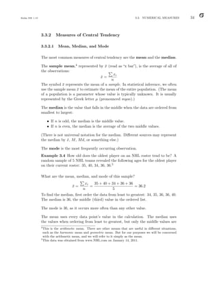
Example 5.2 Suppose you purchase a novelty coin that has a probability of 0.6
of coming up heads when tossed. Let X represent the number of heads when
this coin is tossed twice. The probability distribution of X is:
x 0 1 2
p(x) 0.16 0.48 0.36
Q: What is the expected value of X?
E(X) =
X
all x
xp(x)
= 0 · 0.16 + 1 · 0.48 + 2 · 0.36
= 1.2
On average, in 2 tosses heads will come up 1.2 times.

Suppose we were to repeatedly sample values of X from this distribution. The
law of large numbers (first discussed in Section 4.7) tells us that the proportion
of times each value of X occurs will tend toward its probability of occurring as
the sample size increases. The law of large numbers also tells us that the average
value of X will tend toward the expectation of X as the sample size increases.
Figure 5.2 illustrates the probability distribution of X and a relative frequency
histogram of 1 million sampled values of X. The average of these 1 million
observations is very close to the expectation of X.
0 1 2
0.0
0.1
0.2
0.3
0.4
0.5
0.16
0.48
0.36
p(x)
x
(a) The probability distribution of X.
E(X) = 1.2.
0 1 2
0.0
0.1
0.2
0.3
0.4
0.5
0.159583
0.480965
0.359452
Relative
Frequency
x
(b) Relative frequencies of 1 million simu-
lated values. X̄ = 1.199869.
Figure 5.2: The probability distribution of X and a relative frequency histogram
of 1 million sampled values.
Q: What is the variance of X?
σ2
= V ar(X) =
X
all x
(x − µ)2
p(x)
= (0 − 1.2)2
· 0.16 + (1 − 1.2)2
· 0.48 + (2 − 1.2)2
· 0.36
= 0.48
The standard deviation is σ =
√
0.48.
The true variance of this distribution is 0.48. For the very large sample of 1
million observations illustrated in Figure 5.2b, s2 = 0.4791 (the sample variance
is very close to the theoretical variance).
To develop a feel for the meaning of the mean and standard deviation, it can
help to view a few different distributions. Figure 5.3 illustrates four probability
distributions and their means and standard deviations.

0 1 2 3 4 5 6 7 8 9
0.0
0.1
0.2
0.3
0.4
0.5
p(x)
µ
σ = 4.3
0 1 2 3 4 5 6 7 8 9
0.0
0.1
0.2
0.3
0.4
0.5
p(x)
µ
σ = 1.1
0 1 2 3 4 5 6 7 8 9
0.0
0.1
0.2
0.3
0.4
0.5
p(x)
µ
σ = 2.9
0 1 2 3 4 5 6 7 8 9
0.0
0.1
0.2
0.3
0.4
0.5
p(x)
µ
σ = 2.4
Figure 5.3: Four discrete probability distributions and their means and standard
deviations. Values of the random variable X are given on the horizontal axes.
5.3.1.2 Properties of Expectation and Variance
In Section 3.5, we investigated the effect of a linear transformation (multiplying
by a constant and/or adding a constant) on sample statistics. In this section we
will investigate the effect of a linear transformation on the mean and variance of
a random variable. (Not too surprisingly, a linear transformation has essentially
the same effect here.) All relationships in this section hold for both discrete and
continuous random variables.
For constants a and b:
E(a + bX) = a + bE(X)
(In alternative notation, we could write this as: µa+bX = a+bµX.) This property
is not hard to show using a little algebra on the formula for the expectation of a
discrete random variable.
But recall that an additive constant does not affect the variability:
V ar(a + bX) = b2
V ar(X)
SD(a + bX) = |b|SD(X)
(In alternative notation, σ2
a+bX = b2σ2
X and σa+bX = |b| σX.)

Example 5.3 Recall Example 5.2, in which we found the distribution of the
number of heads (X) in two tosses of a biased coin that comes up heads with
probability 0.6:
x 0 1 2
p(x) 0.16 0.48 0.36
We found that µX = 1.2, σ2
X = 0.48 and σX =
√
0.48.
Suppose you have a friend that likes to gamble, and he offers you the following
deal. If you give him $11, he will toss the coin twice and give you $10 each
time heads comes up. If you choose to take this deal, what are the expectation,
variance, and standard deviation of your winnings?
Let W be a random variable representing your profit in this game (if you lose
money, W will be negative). Then W = −11 + 10X, and the distribution of W
is:
w −11 −1 9
p(w) 0.16 0.48 0.36
We can use the formulas for the mean and expectation of a discrete random
variable to find:
E(W) =
X
all w
wp(w)
= −11 · 0.16 + (−1)0.48 + 9 · 0.36
= 1
On average, you will win $1 in this game.
V ar(W) =
X
all w
(w − µW )2
p(w)
= (−11 − 1)2
· 0.16 + (−1 − 1)2
· 0.48 + (9 − 1)2
· 0.36
= 48
So σ2
W = 48 and σW =
√
48.
But we did not need to carry out these calculations to find the expectation and
variance of the profit, since the profit is simply a linear function of the random
variable X (the number of times heads comes up), and we have already worked

out the mean and variance of X.
E(W) = E(−11 + 10X)
= −11 + 10E(X)
= −11 + 10 · 1.2
= 1
V ar(W) = V ar(−11 + 10X)
= 102
V ar(X)
= 102
· 0.48
= 48
So σ2
W = 48 and σW =
√
48. These are the values that we found above using
the formulas for the mean and variance of a discrete random variable.
Knowing the effect of a linear transformation on the expectation and variance
comes in handy from time to time.
Let’s now investigate a few properties involving the addition and subtraction of
random variables.
If X and Y are two random variables:
• X and Y are independent if knowing the value of one variable gives no
information about the value of the other. (There are formal mathematical
definitions of independence of random variables that are analogous to the
definition of independent events in probability. But in this text the concept
is more important than the formal definition.)
• E(X+Y ) = E(X)+E(Y ). (In the alternative notation: µX+Y = µX +µY .)
This relationship (the mean of the sum is the sum of the means) is true
regardless of whether X and Y are independent.
• E(X − Y ) = E(X) − E(Y )
•
V ar(X + Y ) = V ar(X) + V ar(Y ) + 2 · Cov(X, Y )
V ar(X − Y ) = V ar(X) + V ar(Y ) − 2 · Cov(X, Y )
where Cov(X, Y ) represents the covariance between X and Y . The co-
variance is a measure of the linear relationship between X and Y. We will

not formally define covariance at this point, since we will deal mainly with
the situation in which X and Y are independent. If X and Y are inde-
pendent, their covariance is equal to 0, and the situation is considerably
simpler:
V ar(X + Y ) = V ar(X) + V ar(Y )
V ar(X − Y ) = V ar(X) + V ar(Y )
There is no typo in that last line—the variance of the sum of two independent
random variables is equal to the variance of the difference of those two random
variables.
These notions extend to sums of more than two random variables. If we let
X1, X2, . . . , Xn represent n random variables, then:
E(
X
Xi) =
X
E(Xi)
(The expectation of a sum is the sum of the expectations.)
If in addition X1, X2, . . . , Xn are independent, then:
V ar(
X
Xi) =
X
V ar(Xi)
(If random variables are independent, the variance of their sum is the sum of
their variances.)
Example 5.4 Weights of adult males in the United States have a mean of ap-
proximately 88.7 kg and a standard deviation of approximately 20.1 kg. Weights
of adult females in the United States have a mean of approximately 75.4 kg, and
a standard deviation of approximately 20.5 kg.3
Q: Suppose one adult male and one adult female are randomly and indepen-
dently sampled from the United States population. If the female’s weight is
subtracted from the male’s weight, what are the mean and standard deviation
of the difference in weights?
A: Let X represent the weight of the randomly selected male, and Y represent
the weight of the randomly selected female. X and Y are random variables with
the following means and standard deviations:
3
Although it is impossible to know the true mean and standard deviation of weights of adult
males and females in the United States, these values are close to reality and we will assume
them to be correct for this example. These values are based on information from Fryar et al.
(2012). Anthropometric reference data for children and adults: United states, 2007–2010.
National Center for Health Statistics. Vital Health Stat., 11(252).

µX = 88.7, σX = 20.1
µY = 75.4, σY = 20.5
The difference X − Y is a random variable, with an expectation of:
E(X − Y ) = E(X) − E(Y )
= 88.7 − 75.4
= 13.3
(In alternative notation, µX−Y = 13.3.) On average, the male will weigh 13.3 kg
more than the female.
To find the standard deviation of the difference X − Y , first find the variance
then take the square root. Since X and Y are independent random variables
(due to the nature of the sampling), the variance of their sum or difference is the
sum of their individual variances:
V ar(X − Y ) = V ar(X) + V ar(Y )
= 20.12
+ 20.52
= 824.26
(In alternative notation, σ2
X−Y = 824.26.) The standard deviation of the differ-
ence is σX−Y =
√
824.26 = 28.7.
Q: Suppose we draw three adult males randomly and independently from the
population of the United States. What are the mean and standard deviation of
their total weight?
A: Let X1, X2, X3 be random variables representing the weights of three ran-
domly selected adult men. Their total (X1 +X2 +X3) is a random variable with
expectation:
E(X1 + X2 + X3) = E(X1) + E(X2) + E(X3)
= 88.7 + 88.7 + 88.7
= 266.1
(The mean of the total weight of three randomly selected males is 266.1 kg.)
To find the standard deviation of the total weight, first find the variance then
take the square root. Since X1, X2, X3 are independent random variables, the
variance of their sum is the sum of their variances:
V ar(X1 + X2 + X3) = V ar(X1) + V ar(X2) + V ar(X3)
= 20.12
+ 20.12
+ 20.12
= 1212.03

Balka ISE 1.10 5.4. THE BERNOULLI DISTRIBUTION 110
The standard deviation of the total weight is σX1+X2+X3 =
√
1212.03 = 34.81.
Why would we care about the mean and standard deviation of the total weight
of a number of adults? The mean and standard deviation of the total weight of a
number of adults is an important factor in certain scenarios, such as estimating
the appropriate amount of fuel required for an airline flight, or in constructing a
safe patio deck.
This discussion of properties of expectation has been a bit of an aside, but some
of these concepts are important when we discuss discrete probability distribu-
tions. Let’s now get back to the main focus of this chapter, discrete probability
distributions, by looking at some important distributions that are frequently
encountered in practical situations.
5.4 The Bernoulli Distribution
Optional 8msl available for this section:
Introduction to the Bernoulli Distribution (5:02) (http://youtu.be/bT1p5tJwn_0)
Suppose:
• We conduct an experiment a single time.
• There are two possible mutually exclusive outcomes, labelled success and
failure.
• P(Success) = p. (Failure is the complement of success, so P(Failure) =
1 − p.)
Let X = 1 if a success occurs, and X = 0 if a failure occurs. Then the random
variable X has the Bernoulli distribution, with probability mass function:
P(X = x) = px
(1 − p)1−x
for x = 0, 1. (This is a way of writing P(X = 1) = p and P(X = 0) = 1 − p in a
single formula.)
A few examples of Bernoulli random variables:
• The number of heads when a fair coin is tossed once has the Bernoulli
distribution with p = 1
2.
• The number of fours rolled when a balanced six-sided die is rolled once has
the Bernoulli distribution with p = 1
6.
• The number of people with blood type AB negative when a single Canadian
is randomly selected has the Bernoulli distribution with p ≈ 0.005. (About
0.5% of the Canadian population has AB negative blood.)

Balka ISE 1.10 5.5. THE BINOMIAL DISTRIBUTION 111
The mean of a Bernoulli random variable X can be derived using the formula
for the mean of a discrete probability distribution:
E(X) =
X
xp(x)
= 0 × p0
(1 − p)1−0
+ 1 × p1
(1 − p)1−1
= p
To derive the variance, it is helpful to use the relationship
σ2
= E[(X − µ)2
] = E(X2
) − [E(X)]2
Since we have already found E(X), we now require E(X2):
E(X2
) =
X
x2
p(x)
= 02
× p0
(1 − p)1−0
+ 12
× p1
(1 − p)1−1
= p
Thus
σ2
= E(X2
) − [E(X)]2
= p − p2
= p(1 − p)
Some other common discrete probability distributions are built on the assump-
tion of independent Bernoulli trials. (A Bernoulli trial is a single trial on which
we get either a success or a failure.) The subject of the next section is the bi-
nomial distribution, which is the distribution of the number of successes in n
independent Bernoulli trials.
5.5 The Binomial Distribution
An Introduction to the Binomial Distribution (14:11) (http://youtu.be/qIzC1-9PwQo)
The binomial distribution is a very important discrete probability distribution
that arises frequently in practice. Here are some examples of random variables
that have a binomial distribution:
• The number of times heads comes up if a coin is tossed 40 times.
• The number of universal blood donors in a random sample of 25 Canadians.
(Universal blood donors have Type O negative blood.)

• The number of times the grand prize is won if one Lotto 6/49 ticket is
purchased each week for the next 50 years.
Although these situations are different, they are very similar from a probabil-
ity perspective. In each case there are a certain number of trials (40, 25, and
approximately 50*52), and we are interested in the number of times a certain
event occurs (the number of heads, the number of universal blood donors, the
number of times the grand prize is won in Lotto 6/49). If certain conditions
hold, the number of occurrences will be a random variable that has a binomial
distribution.
The binomial distribution is the distribution of the number of successes in n
independent Bernoulli trials. There are n independent Bernoulli trials if:
• There is a fixed number (n) of independent trials.
• Each individual trial results in one of two possible mutually exclusive out-
comes (these outcomes are labelled success and failure).
• On any individual trial, P(Success) = p and this probability remains the
same from trial to trial. (Failure is the complement of success, so on any
given trial P(Failure) = 1 − p.)
Let X be the number of successes in n trials. Then X is a binomial random
variable with probability mass function:
P(X = x) =

n
x

px
(1 − p)n−x
where n
x

=
n!
x!(n − x)!
is the combinations formula, first discussed in Section 4.6
on page 88.
X is a count of the number of successes in n trials, so X can take on the possible
values 0, 1, 2, . . . , n. Since X can take on one of n+1 possible values (a countable
number of values), it is a discrete random variable. (The binomial distribution
is a discrete probability distribution.)
For a binomial random variable, µ = np and σ2 = np(1 − p). Since the binomial
distribution is a discrete probability distribution, the mean and variance can be
derived using the formulas for expectation and variance that were first discussed
in Section 5.3.1.1: E(X) =
P
xp(x) and σ2 = E[(x − µ)2] =
P
(x − µ)2p(x).
With a little algebra it can be shown that these work out to np and np(1 − p),
respectively.
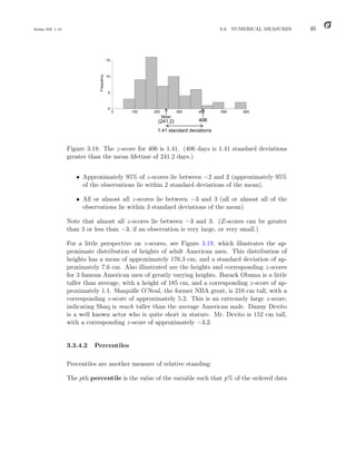
Example 5.5 Suppose a fair coin is tossed 40 times. What is the probability
heads comes up exactly 18 times?

Let the random variable X represent the number of heads in 40 tosses. We need
to find P(X = 18). The probability of getting heads on any single toss is 0.5
(this is what is meant by fair coin). And in most situations it is reasonable to
think that tosses of a coin are independent. So the conditions of the binomial
distribution are satisfied, and:
P(X = 18) =

40
18

0.518
(1 − 0.5)40−18
= 0.1031
Why is P(X = x) = n
x

px(1 − p)n−x the appropriate formula for calculating
probabilities in a binomial setting? Consider an example where we wish to find
the probability of getting exactly two successes in a binomial scenario where
n = 3. Since there are two possible outcomes on any given trial, there are 23 = 8
possible success/failure orderings in three Bernoulli trials. These 8 possibilities
are illustrated in Figure 5.4.
Trial 1
Trial 2
Trial 3
FFF (0 successes)
F
FFS (1 success)
S
F
Trial 3
FSF (1 success)
F
FSS (2 successes)
S
S
F
Trial 2
Trial 3
SFF (1 success)
F
SFS (2 successes)
S
F
Trial 3
SSF (2 successes)
F
SSS (3 successes)
S
S
S
Figure 5.4: The 8 possible success/failure (S/F) orderings in 3 Bernoulli trials.
If there are three trials, then getting exactly two successes can happen in three
different ways (the 2nd, 3rd, and 5th combinations in Figure 5.4). SSF, SFS, and
FSS all individually have the same probability of occurring, p2(1 − p)1.4 But in
binomial scenarios we do not care about the order in which successes and failures
occur, the point of interest is the total number of successes. So we add these
three probabilities together, for a final answer of P(X = 2) = 3 × p2(1 − p)1. In
the general case, we don’t have to go through this and list out all the different
4
The trials are independent, so to find the probability of the events all occurring, we multiply
their individual probabilities together. The probability of SSF is p×p×(1−p) = p2
(1−p), the
probability of SFS is p×(1−p)×p = p2
(1−p), and the probability of FSS is (1−p)×p×p =
p2
(1 − p).

ways of getting x successes in n trials, since that is precisely what n
x

gives
us. (For this example, 3
2

= 3.) In the general case, the probability of any
specific ordering of x successes and n − x failures is px(1 − p)n−x, and n
x

gives
the number of ways x successes and n − x failures can happen. So in the end,
P(X = x) = n
x

px(1 − p)n−x.
5.5.1 Binomial or Not?
Binomial/Not Binomial: Some Examples (8:07) (http://youtu.be/UJFIZY0xx_s)
Students often ask questions along the lines of: “when does a random variable
have a binomial distribution?” The short answer is that a random variable has
a binomial distribution if the conditions for a binomial random variable given
above are satisfied. We will need to be able to recognize that a random variable
has a binomial distribution from the information in a given situation. Let’s look
at a few examples to see what information we should consider.
• A six-sided die is rolled 1,000 times. Let X represent the number of times
that the die comes up with a three on the top face.
Here X is a binomial random variable. Even though there are 6 possibilities
when a die is rolled, we are interested only in the number of threes. So
there are only two events of interest on any given roll: three and not a
three. It is also reasonable to assume independence between rolls of a die,
so the binomial conditions are perfectly justified here.
• A car manufacturer calls a random sample of 200 purchasers of one of their
models. Let X be the number of people that say they are satisfied with
the car.
As long as it is a random sample and the independence assumption is
reasonable, X is a binomial random variable with n = 200 and an unknown
value of p.
• A room contains 5 males and 5 females. Pick a random sample of size
n = 4 without replacement. Let X represent the number of males in the
sample.
X is not a binomial random variable. Since the sampling is done with-
out replacement, the trials are not independent (the probability a male is
chosen changes from trial to trial, depending on what has occurred pre-
viously). In this scenario, X has the hypergeometric distribution, a

distribution discussed in Section 5.6. Had the sampling been carried out
with replacement, then the trials would be independent, and X would have
a binomial distribution.
• The number of free throws a specific NBA player makes in 100 attempts.
This is debatable. The binomial model would likely be reasonable, but
not perfectly true. There are a fixed number of trials and we are counting
the number of successes—it is the binomial assumptions of independence
and constant probability of success that are a little troubling. If the player
misses 3 shots in a row, say, will this have no effect on his probability of
making the next throw? Some studies have investigated a possible depen-
dence in free throw attempts, and the results show little to no evidence of
dependence. Overall the binomial distribution would likely provide a rea-
sonable approximate model here, though it would not perfectly represent
reality.
5.5.2 A Binomial Example with Probability Calculations
Example 5.6 According to the Canadian Dermatology Association, approxi-
mately 20% of newborn babies have “baby acne” (acne neonatorum).5
Q: If 25 newborn babies are randomly selected, what is the probability that
exactly one has baby acne?
A: Here the conditions of the binomial distribution are satisfied. There are a
fixed number of trials (25 babies are selected), each one can be labelled as a
success or a failure (success: the baby has acne), the trials are independent (the
babies are randomly selected), and the probability of success is constant (each
randomly selected baby has a 20% chance of having baby acne). So this is a
straightforward binomial problem with n = 25, p = 0.20:
P(X = 1) =

25
1

0.201
(1 − 0.20)25−1
= 0.0236
The binomial probabilities for this problem are illustrated in Figure 5.5.
Q: What is the probability that at least one of the 25 babies has baby acne?
A: P(X ≥ 1) = P(X = 1) + P(X = 2) + . . . + P(X = 25). This would be very
cumbersome to carry out by hand, as it would require calculating 25 binomial
5
http://www.dermatology.ca/skin-hair-nails/skin/acne/baby-acne/. Accessed February
18, 2014.

0 2 4 6 8 10 12 14 16 18 20 22 24
Number with Baby Acne
Probability
0.00
0.05
0.10
0.15
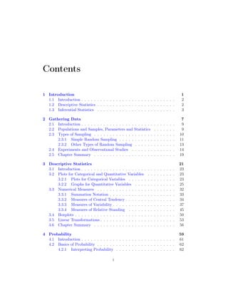
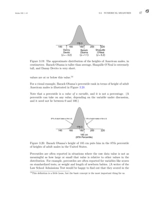
Figure 5.5: The distribution of the number of babies with baby acne in a sample
of 25 newborns (a binomial distribution with n = 25, p = 0.20).
probabilities and adding them. The required probability is much easier to calcu-
late if we realize that the only possibility other than X ≥ 1 is X = 0 (X = 0 is
the complement of X ≥ 1), and thus:
P(X ≥ 1) = 1 − P(X = 0) = 1 − [

25
0

0.200
(1 − 0.20)25
] = 0.996
Q: If 50 newborn babies are randomly selected, what is the probability that at
least 10 have baby acne?
A: P(X ≥ 10) = P(X = 10)+P(X = 11)+. . .+P(X = 50). These probabilities
are illustrated in Figure 5.6. Solving this problem would involve calculating 41
binomial probabilities and adding them. It would be a little easier to work in the
other direction: P(X ≥ 10) = 1 − P(X ≤ 9). But we’d still need to calculate
10 binomial probabilities and add them: P(X ≤ 9) = P(X = 0) + P(X =
1) + . . . + P(X = 9). It is best to use software to answer this type of question.6
The correct answer is 0.556.
A note on terminology: the cumulative distribution function, F(x), is de-
fined as: F(x) = P(X ≤ x), where X represents the random variable X, and
x represents a value of X. For example, we may be interested in the probability
that X takes on a value less than or equal to 10: F(10) = P(X ≤ 10). Text-
books often contain tables giving the cumulative distribution function for some
distributions, and statistical software has commands that yield the cumulative
distribution function for various distributions.7
6
In R, the command 1 − pbinom(9, 50, .2) yields P(X ≥ 10) = 0.556.
7
In R, the command pbinom calculates the cumulative distribution function for the binomial
distribution.

Balka ISE 1.10 5.6. THE HYPERGEOMETRIC DISTRIBUTION 117
0 2 4 6 8 10 12 14 16 18 20 22 24 26 28 30
Number with Baby Acne
Probability
0.00
0.02
0.04
0.06
0.08
0.10
0.12
Figure 5.6: The shaded area represents P(X ≥ 10) for n = 50, p = 0.2.
Example 5.7 (A statistical inference type of problem.)
Suppose it is believed that in a certain area, 30% of the population has latent
tuberculosis (they carry the bacterium Mycobacterium tuberculosis, but do not
have active tuberculosis).8 In a random sample of 100 individuals from this area,
it is found that 49 have latent tuberculosis. Does this provide strong evidence
that the percentage of individuals in this area with latent tuberculosis is greater
than 30%?
Suppose for a moment that the true percentage of this population that has latent
tuberculosis is in fact 30%. What is the probability of observing 49 or more
with latent tuberculosis in a sample of 100 individuals? If the true rate is 30%,
then the number that have latent tuberculosis in a sample of 100 will have a
binomial distribution with n = 100 and p = 0.30. We can use software to find
P(X ≥ 49) ≈ 0.000052. The probability of observing 49 or more with latent
tuberculosis, if the true rate is 30%, is very small (about 1 in 19,000). This
implies there is very strong evidence that the true rate of latent tuberculosis in
this area is greater than 30%. We will frequently use this type of logic when we
carry out hypothesis tests in later chapters.
5.6 The Hypergeometric Distribution
An Introduction to the Hypergeometric Distribution (15:35) (http://youtu.be/L2KMttDm3aY)
8
According to the World Health Organization, the percentage of the world’s population that
has latent tuberculosis is approximately 30%.

The hypergeometric distribution is related to the binomial distribution, but it
arises in slightly different situations. Like the binomial distribution, the hyper-
geometric distribution is the distribution of the number of successes in n trials.
But unlike binomial distribution scenarios, here the trials are not independent.
Example 5.8 Suppose a room contains four females and 12 males, and three
people are randomly selected without replacement. What is the probability there
are exactly two females in the three people selected?
The number of females in the sample of three people does not follow a binomial
distribution, since the trials are not independent (the probability of selecting a
female changes from trial to trial, depending on what happened on previous tri-
als). For example, the probability the first person selected is female is 4
16 = 0.25,
but for the second person selected:
P(Second person is female|First person is female) =
3
15
= 0.20
P(Second person is female|First person is male) =
4
15
≈ 0.27
Since the probability of drawing a female on any given trial depends on what
has happened on previous trials, the trials are not independent, and the number
of females selected will not follow a binomial distribution. (Had the sampling
been carried out with replacement, the probability of selecting a female would
stay constant at 0.25 and the number of females selected would follow a bino-
mial distribution.) The probability distribution of the number of females in the
without replacement case is called the hypergeometric distribution. We’ll look
at the probability mass function for the hypergeometric distribution below, but
let’s first work out the required probability using a little logic. The probability
of selecting exactly two females in the sample of three people is:
Number of ways 2 females can be chosen from 4 females × Number of ways 1 male can be chosen from 12 males
Total number of ways 3 people can be chosen from the 16 in the room
=
4
2
12
1

16
3
= 0.129
a
x

is the combinations formula—the number of different ways x items can be
chosen from a items, if order of selection is not important.9
9
For example, 4
2

=
4!
2!(4 − 2)!
= 6. In other words, there are 6 different two-female groups that
can be chosen from 4 females. The combinations formula was first encountered in Section 4.6
on page 88.

Had we attempted (mistakenly) to calculate the probability using the bino-
mial distribution with n = 3 and p = 4
16 = 0.25, we would have thought
P(X = 2) = 3
2

0.252(1 − 0.25)1 = 0.14. This is not the correct probability.
Let’s look at a related example that differs in a fundamental way. Suppose a
small arena contains 400 females and 1200 males. Three people are randomly
selected without replacement. What is the probability there are exactly two
females among the three people selected?
We can calculate the required probability using the same logic we used above:
P(X = 2) =
400
2
1200
1

1600
3
= 0.1405
Had we attempted to calculate the probability using the binomial distribution
with n = 3 and p = 4
16 = 0.25, we would have thought P(X = 2) = 3
2

0.252(1 −
0.25)1 = 0.1406. This is not the correct answer, but it is very close. Here the
binomial probability is much closer to the correct probability than in the previous
example. What is the difference between these two scenarios? In the latter
case the sample size represented only a small proportion of the total number
of individuals. When that is the case, the probability of success changes only
a small amount from trial to trial, depending on the outcomes of the previous
trials, and the binomial distribution provides a close approximation to the correct
probability. As a rough guideline, the binomial distribution provides a reasonable
approximation to the hypergeometric distribution if we are not sampling more
than 5% of the total population.
Now that we’ve discussed the motivation for the hypergeometric distribution,
let’s look at a slightly more formal introduction. Suppose we are randomly
sampling n objects without replacement from a source that contains a successes
and N − a failures. (There is a total of N objects.) Let X represent the number
of successes in the sample. Then X has the hypergeometric distribution:
P(X = x) =
a
x
N−a
n−x

N
n

for x = Max(0, n + a − N), . . . , Min(a, n). Min(a, n) is notation representing the
minimum of a and n. The random variable X cannot take on values greater than
the sample size n, or values greater than the total number of successes a. Nor
can it take on values less than 0, or less than the difference between the sample
size and number of failures.

For the hypergeometric distribution, µ = n a
N and σ2 = n a
N (1 − a
N )N−n
N−1 . Note
that the mean number of successes is the same as when the sampling is done with
replacement (where the binomial distribution applies), but the variance is less.
Example 5.9 Suppose a shipment of 1000 parts arrives at a factory, and it
is known that 40 of these parts are defective (which parts are defective is un-
known). Twenty-five parts are randomly selected without replacement. What is
the probability exactly four of these parts are defective?
In the notation of the hypergeometric distribution, N = 1000, n = 25, a = 40,
and x = 4. The probability of selecting exactly four defective parts is:
P(X = 4) =
40
4
960
21

1000
25
= 0.0128
The distribution of the number of defective parts in this scenario is illustrated
in Figure 5.7.
0 2 4 6 8 10 12 14 16 18 20 22 24
0.0
0.1
0.2
0.3
Probability
Number of Defective Parts
Figure 5.7: Distribution of the number of defective parts in a sample of 25 from
a population containing 40 defective and 960 non-defective parts.
Many people find it easier to carry out the calculations by working through the
logic outlined in the previous examples, and not by relying on the formula.
Example 5.10 The multivariate hypergeometric distribution generalizes the hy-
pergeometric distribution to more than 2 groups of objects. For example, if 7
cards are randomly drawn without replacement from a well-shuffled deck, the
probability there are 4 clubs, 0 hearts, 2 diamonds, and 1 spade drawn is:
P(4 clubs, 0 hearts, 2 diamonds, 1 spade) =
13
4
13
0
13
2
13
1

52
7
= 0.0054

Balka ISE 1.10 5.7. THE POISSON DISTRIBUTION 121
5.7 The Poisson Distribution
5.7.1 Introduction
An Introduction to the Poisson Distribution (9:03) (http://youtu.be/jmqZG6roVqU)
The Poisson distribution often arises as the distribution of the number of oc-
currences of an event in a given unit of time, area, distance, or volume. It can
be a useful model when events can be thought of as occurring randomly and
independently through time (or area, or volume).
Here are some examples of random variables that have been modelled by a Pois-
son distribution:
• The number of calls arriving at a switchboard in a minute.
• The number of chocolate chips in a cookie.
• The number of bacteria per ml of a solution.
• The number of radioactive decays of a substance in a one second period.
The random variables in these examples may or may not have a Poisson distri-
bution, as specific conditions need to hold in order for a random variable to have
this distribution. The following conditions are phrased in terms of time, but it
would be equally applicable to a situation involving volume, area, or distance.
If:
• Events are occurring independently in time. (Knowing when one event
occurs gives no information about when another event will occur.)
• The probability that an event occurs in a given length of time does not
change through time. (The theoretical rate of events stays constant through
time.)
Then X, the number of events in a fixed unit of time, has a Poisson distribution
with probability mass function:
P(X = x) =
λxe−λ
x!
for x = 0, 1, 2, . . . (The random variable X can take on a countably infinite
number of possible values, and is therefore a discrete random variable.)
The parameter λ represents the theoretical mean number of events in the time
period under discussion. (Some sources use µ in place of λ in the formula.)

For a Poisson random variable, the mean and variance are both equal to the
parameter λ: µ = λ, σ2 = λ.
The mathematical constant e is the base of natural logarithms (e ≈ 2.71828).
It is an important mathematical constant that, like π, arises in many different
mathematical situations. e is an irrational number, with infinite non-repeating
decimal places. When doing calculations, do not round e, as this may result in
a lot of round-off error. Use the value for e given by your calculator or software.
Example 5.11 A certain volunteer fire department responds to an average of 7
emergencies per month. Suppose that the number of emergency responses in any
given month follows a Poisson distribution with λ = 7. (This would be the case
if the emergencies are occurring randomly and independently, and at a constant
theoretical rate, which is likely a reasonable approximation to the reality of the
situation.) The distribution of the number of emergency responses if λ = 7 is
displayed in Figure 5.8.
0 2 4 6 8 10 12 14 16 18 20 22 24
0.00
0.04
0.08
0.12
Number of Emergency Responses
Probability
Figure 5.8: The distribution of the number of emergency responses in a month.
(A Poisson distribution with λ = 7.)
Q: In a given month, what is the probability that the department responds to
exactly 10 emergencies?
A:
P(X = 10) =
710e−7
10!
= 0.071
These calculations can be carried out on a calculator or using appropriate soft-
ware.10
Q: In a given month, what is the probability that the department responds to
fewer than 3 emergencies?
10
In R, the command dpois(10, 7) would yield the correct probability for this question.

A:
P(X 3) = P(X = 0) + P(X = 1) + P(X = 2)
=
70e−7
0!
+
71e−7
1!
+
72e−7
2!
= 0.0009 + 0.0064 + 0.0223
= 0.0296
The probabilities are illustrated in Figure 5.9. We can carry out these calculations
by hand, but we could save ourselves a little time by using software.11
0 2 4 6 8 10 12 14 16 18 20 22 24
0.00
0.04
0.08
0.12
Number of Emergency Responses
Probability
Figure 5.9: The shaded area represents P(X 3).
5.7.2 The Relationship Between the Poisson and Binomial Dis-
tributions
Optional 8msl videos available for this section:
The Relationship Between the Binomial and Poisson Distributions (5:23) (http://youtu.be/eexQyHj6hEA)
Proof that the Binomial Distribution tends to the Poisson Distribution (5:25) (http://youtu.be/ceOwlHnVCqo)
There is an important relationship between the binomial and Poisson distribu-
tions:
The binomial distribution with parameters n and p tends toward the Poisson
distribution with λ = np as n → ∞, p → 0 and λ = np stays constant.
11
In R, the command ppois(2, 7) would yield the correct probability. The ppois command
yields the cumulative distribution function for the Poisson distribution (ppois(2, 7) calculates
P(X ≤ 2)).

An implication of this is that the Poisson distribution with λ = np closely ap-
proximates the binomial distribution if n is large and p is small.
Example 5.12 Cystic fibrosis is a genetic disorder that causes thick mucus to
form in the lungs and other organs. Approximately 1 in every 2,500 Caucasian
babies is born with cystic fibrosis. In a random sample of 500 Caucasian babies,
what is the probability that exactly 2 have cystic fibrosis?
The number of babies with cystic fibrosis will have a binomial distribution with
n = 500 and p = 1
2500. We can find the probability that two babies have cystic
fibrosis using the binomial probability mass function:
P(X = 2) =

500
2

(
1
2500
)2
(1 −
1
2500
)498
= 0.01635
Since n is large (500) and p is small ( 1
2500), the probability calculated using the
Poisson approximation would closely approximate this exact probability. The
Poisson approximation with λ = np = 500 × 1
2500 = 0.20:
P(X = 2) =
0.202e−0.20
2!
= 0.01637
The Poisson distribution very closely approximates the binomial distribution in
this example.
Another example of the Poisson approximation to the binomial occurs in the
radioactive decay of a substance. A radioactive decay occurs when an individual
atom emits a particle of radiation. Even a small amount of a substance contains
a very large number of atoms, and the probability that any individual atom
experiences a radioactive decay in a short time period is usually very small. If
the radioactive decays of a substance are being counted, then the number of
decays in a given time period would have a binomial distribution with a very
large n and a very small p, and the Poisson distribution would therefore provide
an excellent approximation.
Why would we ever use the Poisson approximation to the binomial, and not sim-
ply use the binomial distribution? It is usually better to use the exact distribution
rather than an approximation (when possible). But for large n, calculating bino-
mial probabilities can be problematic. (The relevant factorials and the binomial
coefficient may be too large for a calculator to handle.) In these cases it might
be more convenient to calculate an approximation based on the Poisson distri-
bution. In addition, in some situations that are truly binomial in their nature,
we may know the mean number of events but not the values of n and p. Poisson

probabilities can be calculated from only the mean number of occurrences, but
calculating binomial probabilities requires the values of both n and p. In the
radioactive decay scenario, we may have a good estimate of the mean number of
radioactive decays in a certain time period, but not the exact number of atoms
and the probability an atom decays. In this situation we would need to use the
Poisson approximation.
5.7.3 Poisson or Not? More Discussion on When a Random
Variable has a Poisson distribution
Poisson or Not? (When does a random variable have a Poisson distribution?) (14:40)
(http://youtu.be/sv_KXSiorFk)
It can be difficult to determine if a random variable has a Poisson distribution.
It is usually straightforward to determine if a random variable is a count of the
number of events in a given time period (or area, distance, volume, etc.), but the
other conditions (such as independently occurring events) are often much more
difficult to assess.
The Poisson distribution’s relationship with the binomial distribution can some-
times help us determine if a random variable has (approximately) a Poisson
distribution. If the underlying reality can be envisioned as a large number of
independent trials, each with a small probability of success (as in the radioactive
decay scenario outlined in the previous section), then the Poisson model may very
well be reasonable. The Poisson model may provide a reasonable approximation
even if there is weak dependence between the trials.
Let’s look at a few plots that may help us visualize when a random variable has
a Poisson distribution. Consider the three scenarios illustrated in Figure 5.10,
which give different patterns of events over an area. In all three cases we are
counting the number of events in a randomly selected square area, but only one
specific scenario leads to the Poisson distribution.

(a) Events are distributed randomly and independently
across the plot, at a constant theoretical rate. We might
see a pattern like this if we were observing where rain-
drops fell on a piece of paper. The number of events
in a randomly selected square would follow a Poisson
distribution.
(b) The events are clumped together. We might see a pat-
tern like this when observing the location of cows in a field.
The events are not occurring randomly and independently
with the same theoretical rate across the plot. The number
of events in a randomly selected square would not follow a
Poisson distribution.
(c) The events are evenly distributed across the plot. We
might see a pattern like this if observing the location of
street lights in a large parking lot. The number of events
in a randomly selected square would not follow a Poisson
distribution.
Figure 5.10: Three scenarios representing different distributions of events over an
area. In all three situations, the number of events in a randomly selected square
has a theoretical mean of about 1.4, but only the top scenario would result in a
Poisson distribution.

Balka ISE 1.10 5.8. THE GEOMETRIC DISTRIBUTION 127
Let’s look at another example. Consider two related questions:
• Would the number of fatal plane crashes in a year for U.S. airlines have a
Poisson distribution?
• Would the number of fatalities (deaths) in plane crashes in a year for U.S.
airlines have a Poisson distribution?
There are millions of flights each year, and each one of them has a very tiny
probability of experiencing a fatal crash. These factors might lead us to consider
the Poisson distribution, as it may well approximate the binomial distribution in
this setting. (Also, to a reasonable approximation, fatal crashes can be thought
of as occurring randomly and independently.) So the number of fatal crashes in
a given time period would likely follow a Poisson distribution. But accurately
estimating λ would be difficult, as there are many factors that change through
time (such as technology, airline safety standards, and the number of flights).
All in all, the Poisson distribution would probably be a reasonable model for
the number of fatal crashes in a given time period, but we could only roughly
estimate λ.
On the other hand, the number of fatalities would definitely not have a Poisson
distribution, since fatalities do not not occur independently. When there is a
fatal crash, it often involves a large number of fatalities, leading to large spikes
in the number of deaths in a given year.
Consider the plots in Figure 5.11, which illustrate the number of fatal crashes
and number of fatalities for U.S. commercial airlines for the years 1982–2012.12
Although at a casual glance these plots might look similar, there are important
differences. If we focus on the number of fatalities, there are 0 in five of the
years, but there are massive spikes to over 400 in two of them. (One of these
years was 2001, in which American Airlines flight 587 crashed and all 260 people
on board were killed.) A Poisson model simply cannot handle situations where
observing 0 events is a likely outcome, but observing several hundred events is
also reasonably likely as well.
5.8 The Geometric Distribution
Introduction to the Geometric Distribution (10:48)
(http://youtu.be/zq9Oz82iHf0)
12
The data was summarized from the National Transportation Safety Board website: http:
//www.ntsb.gov/data/paxfatal.html. Accessed December 10, 2013.

1982 1990 2000 2012
0
1
2
3
4
5
Crashes
(a) Fatal crashes for United States airlines from 1982-2012.
1982 1990 2000 2012
0
200
400
Fatalities
(b) Fatalities for United States airlines from 1982-2012.
Figure 5.11: The number of fatal crashes and number of fatalities for United
States airlines for the years 1982–2012. The number of crashes in a year would
roughly follow a Poisson distribution (but λ would change through time). The
number of fatalities would not follow a Poisson distribution.
The geometric distribution arises as the distribution of the number of trials
needed to get the first success in repeated independent Bernoulli trials.
A few examples of random variables that could be modelled with a geometric
distribution:
• The number of tosses needed to get heads for the first time in repeated
tosses of a coin.
• The number of phone calls a telemarketer must make to get their first sale.
• The number of people needed to be sampled to get the first person with
blood type AB.
For a geometric distribution to arise, there must be repeated independent Bernoulli
trials with a constant probability of success. In other words:
• There are repeated independent trials.

comes (labelled success and failure).
If we let X represent the number of trials needed to get the first success, then
X is a random variable that has the geometric distribution.
Let’s develop the probability mass function for the geometric distribution. In
order for the first success to occur on the xth trial, two events must occur:
1. The first x − 1 trials must be failures, which has probability (1 − p)x−1.
2. The xth trial must be a success, which has probability p.
The probability mass function is given by the product of these two probabilities:
P(X = x) = p(1 − p)x−1
for x = 1, 2, 3, . . .
For the geometric distribution, µ =
1
p
and σ2 =
1 − p
p2
.
Example 5.13 An American roulette wheel consists of 18 red slots, 18 black
slots, and 2 green slots. In the game of roulette, the wheel is spun and a ball
lands randomly in one of the slots. Each of the slots can be considered equally
likely. If a player repeatedly bets $1 on black, what is the probability that their
first win comes on the sixth spin of the wheel? (The player wins if the ball lands
in a black slot.)
Since we are interested in how many trials (spins) it takes for the ball to land
in a black slot for the first time, a success will be the ball landing in a black
slot. A failure will be the ball landing in a red or green slot (any slot but black).
On any given trial, P(Success) = Number of black slots
Total number of slots = 18
38. As long as the trials
are independent, which is a pretty reasonable assumption in this case, we have
repeated independent Bernoulli trials with a constant probability of success of
p = 18
38. The probability the first success occurs on the sixth trial is:
P(X = 6) =
18
38
(1 −
18
38
)5
= 0.0191
The distribution of the number of spins needed to get the first win is illustrated
in Figure 5.12.

1 2 3 4 5 6 7 8 9 10 11 12
0.0
0.1
0.2
0.3
0.4
Probability
Trial Number of First Win
Figure 5.12: The distribution of the number of trials needed to get the first win
when betting on black in American roulette (truncated at x = 12). The geometric
distribution always has a mode at x = 1, with the probabilities decreasing as x
increases.
A nice feature of the geometric distribution is that the cumulative distribution
function is of relatively simple form:13
F(x) = P(X ≤ x) = 1 − (1 − p)x
for x = 1, 2, 3, . . .
Example 5.14 Suppose a player is betting on black on repeated spins of Amer-
ican roulette, as in Example 5.13. What is the probability their first win comes
on or before the 3rd spin?
We could find the answer by calculating 3 geometric probabilities and adding
them:
P(X ≤ 3) = P(X = 1) + P(X = 2) + P(X = 3)
= p(1 − p)0
+ p(1 − p)1
+ p(1 − p)2
=
18
38
+ (
18
38
)(1 −
18
38
) + (
18
38
)(1 −
18
38
)2
= 0.8542
This method will result in the correct probability, but we could have saved our-
13
To show this, first note that P(X ≤ x) = 1−P(X x). A geometric random variable X will
take on a value greater than x if the first x trials are failures, which has probability (1 − p)x
.
So F(x) = P(X ≤ x) = 1 − (1 − p)x
.

Balka ISE 1.10 5.9. THE NEGATIVE BINOMIAL DISTRIBUTION 131
selves a little work by using the formula for the cumulative distribution function:
P(X ≤ x) = 1 − (1 − p)x
P(X ≤ 3) = 1 − (1 −
18
38
)3
= 0.8542
5.9 The Negative Binomial Distribution
Introduction to the Negative Binomial Distribution (7:33) (http://youtu.be/BPlmjp2ymxw)
The negative binomial distribution is a generalization of the geometric distri-
bution. The geometric distribution is the distribution of the number of trials
needed to get the first success in repeated independent Bernoulli trials, and the
negative binomial distribution is the distribution of the number of trials needed
to get the rth success.14 (r represents a number of successes, so it must be a
positive whole number.)
A few examples of random variables that could be modelled with a negative
binomial distribution:
• The number of tosses needed to get heads for the seventh time in repeated
tosses of a coin.
• The number of new cars that must be sampled to get 12 with no observable
paint defects.
• The number of people needed to be sampled to get 25 people with diabetes.
For a negative binomial distribution to arise, there must be repeated independent
Bernoulli trials with a constant probability of success, as described in Section 5.8.
In order for the rth success to occur on the xth trial, two events must occur:
1. The first x − 1 trials must result in r − 1 successes. The probability of this
can be found using the binomial probability mass function: x−1
r−1

pr−1(1 − p)(x−1)−(r−1)
2. The xth trial must be a success, which has probability p.
Since the trials are independent, the probability that the rth success occurs on
14
A negative binomial random variable can be defined in a variety of different ways. For
example, it is sometimes defined as the number of failures before getting the rth success. But
we will use the definition given here.

Balka ISE 1.10 5.9. THE NEGATIVE BINOMIAL DISTRIBUTION 132
the xth trial is the product of these two probabilities:
P(X = x) = p ×

x − 1
r − 1

pr−1
(1 − p)(x−1)−(r−1)
=

x − 1
r − 1

pr
(1 − p)x−r
For x = r, r + 1, . . .
For the negative binomial distribution, µ =
r
p
and σ2 =
r(1 − p)
p2
.
Consider again the information in Example 5.13. An American roulette wheel
contains 18 red slots, 18 black slots, and 2 green slots. In the game of roulette,
the wheel is spun and a ball lands randomly in one of the slots. Each of the slots
can be considered equally likely. If a player repeatedly bets $1 on black, what is
the probability that their fourth win comes on the 16th spin of the wheel?
As discussed in Example 5.13, here there are repeated independent Bernoulli
trials, with P(Success) = 18
38 on any given trial. The number of spins needed to
get the fourth win has the negative binomial distribution with r = 4 and p = 18
38.
The probability the fourth win occurs on the 16th spin is:
P(X = 16) =

x − 1
r − 1

pr
(1 − p)x−r
=

16 − 1
4 − 1

(
18
38
)4
(1 −
18
38
)16−4
= 0.0103
The distribution of the number of spins needed to get the fourth win is illustrated
in Figure 5.13.
A random variable that has a negative binomial distribution can sometimes be
mistaken for a random variable that has a binomial distribution. A binomial
distribution results from a fixed number of trials (n) where we are interested
in the number of successes (the random variable X ). The negative binomial
distribution results when the number of successes (r) is a fixed number, and the
number of trials required to reach that number of successes is a random variable
(X).

Balka ISE 1.10 5.10. THE MULTINOMIAL DISTRIBUTION 133
4 6 8 10 12 14 16 18 20 22 24 26 28 30
0.00
0.05
0.10
0.15
Probability
Trial Number of Fourth Win
Figure 5.13: The distribution of the number of spins needed to get the fourth
win when betting on black in American roulette (truncated at x = 30).
5.10 The Multinomial Distribution
Introduction to the Multinomial Distribution (11:15) (http://youtu.be/syVW7DgvUaY)
The multinomial distribution is a generalization of the binomial distribution. In
a binomial setting, there are n Bernoulli trials, where on each trial there are two
possible outcomes (success and failure). In a multinomial setting, the number of
possible outcomes on each trial is allowed to be greater than two.
Example 5.15 The distribution of blood types in the U.S. population is given
in Table 5.3.
Type O A B AB
Probability 0.44 0.42 0.10 0.04
Table 5.3: The distribution of ABO blood types in the United States population.
The multinomial distribution can help us answer a question like: In a random
sample of 25 Americans, what is the probability that 10 have Type O, 10 have
Type A, 3 have Type B, and 2 have Type AB?
In order for the multinomial distribution to arise, several conditions must hold:
• There are n independent trials.
• Each trial results in one of k mutually exclusive and exhaustive outcomes.
• On any single trial, these k outcomes occur with probabilities p1, . . . , pk.
(Since one of these k mutually exclusive outcomes must occur,
Pk
i=1 pi =
1.)

Balka ISE 1.10 5.10. THE MULTINOMIAL DISTRIBUTION 134
• The probabilities stay constant from trial to trial.
If we let the random variable Xi represent the number of occurrences of outcome
i, (i = 1, . . . , k), then:
P(X1 = x1, . . . , Xk = xk) =
n!
x1! · · · xk!
px1
1 · · · pxk
k
for xi = 0, 1, . . . , n, and
Pk
i=1 xi = n.
When viewed in isolation, each Xi is a random variable that has a binomial
distribution. So E(Xi) = npi and V ar(Xi) = npi(1 − pi). Together, these k
random variables have the multinomial distribution.
Let’s return to the distribution of blood types in the United States and answer
the question posed above.
Type O A B AB
Probability 0.44 0.42 0.10 0.04
In a random sample of 25 Americans, what is the probability that 10 have Type
O, 10 have Type A, 3 have Type B, and 2 have Type AB?
Let X1 represent the number of people in the sample with blood type O, X2
represent the number with blood type A, X3 represent the number with blood
type B, and X4 represent the number with blood type AB. From the table,
p1 = 0.44, p2 = 0.42, p3 = 0.10, p4 = 0.04. The required probability can be found
using the multinomial distribution probability mass function:
P(X1 = x1, . . . , Xk = xk) =
n!
x1! · · · xk!
px1
1 · · · pxk
k
P(X1 = 10, X2 = 10, X3 = 3, X4 = 2) =
25!
10!10!3!2!
0.4410
0.4210
0.103
0.042
= 0.0073

5.11 Chapter Summary
In this chapter we discussed discrete random variables and discrete probability
distributions. Discrete random variables can take on a countable number of
possible values (which could be either finite or infinite). This differs from a
continuous random variable in that a continuous random variable takes on an
infinite number of possible values, corresponding to all possible values in an
interval.
To find the expectation of a function of a discrete random variable X (g(X), say):
E[g(X)] =
X
all x
g(x)p(x)
The expected value of a random variable is the theoretical mean of the random
variable. For a discrete random variable X:
E(X) = µX =
X
xp(x)
The variance of a discrete random variable X is:
σ2
X = E[(X − µ)2
] =
X
all x
(x − µ)2
p(x)
A useful relationship: E[(X − µ)2] = E(X2) − [E(X)]2
For constants a and b: E(a + bX) = a + bE(X), σ2
a+bX = b2σ2
X, σa+bX = |b| σX
If X and Y are two random variables:
E(X + Y ) = E(X) + E(Y )
E(X − Y ) = E(X) − E(Y )
σ2
X+Y = σ2
X + σ2
Y + 2 · Covariance(X, Y )
σ2
X−Y = σ2
X + σ2
Y − 2 · Covariance(X, Y )
If X and Y are independent, their covariance is equal to 0, and things simplify
a great deal:
σ2
X+Y = σ2
X + σ2
Y
σ2
X−Y = σ2
X + σ2
Y

There are some common discrete probability distributions, such as the binomial
distribution, the hypergeometric distribution, and the Poisson distribution.
The binomial distribution is the distribution of the number of successes in n
independent Bernoulli trials. There are n independent Bernoulli trials if:
• There is a fixed number (n) of independent trials.
comes (these outcomes are labelled success and failure).
Let X be the number of successes in n trials. Then X is a binomial random
variable with probability mass function: P(X = x) = n
x

px(1 − p)n−x
The hypergeometric distribution is related to the binomial distribution, but arises
in slightly different situations. Suppose we are randomly sampling n objects with-
out replacement from a source that contains a successes and N −a failures. Let X
represent the number of successes in the sample. Then X has the hypergeometric
distribution:
P(X = x) =
a
x
N−a
n−x

N
n
, for x = Max(0, n + a − N), . . . , Min(a, n).
If the sampling were carried out with replacement, then the binomial distribution
would be the correct probability distribution. If the sampling is carried out
without replacement, but the number sampled (n) is only a small proportion of
the total number of objects (N), then the probability calculated based on the
binomial distribution would be close to the correct probability calculated based
on the hypergeometric distribution.
Certain conditions need to be true in order for a random variable to have a
Poisson distribution. Suppose we are counting the number of occurrences of an
event in a fixed unit of time, and events can be thought of as occurring randomly
and independently in time. Then X, the number of occurrences in a fixed unit
of time, has a Poisson distribution:
P(X = x) =
λxe−λ
x!
There is a relationship between the binomial and Poisson distributions. As n →
∞ and p → 0, while λ = np is constant, the binomial distribution tends toward

the Poisson distribution. In practice, this means that we can use the Poisson
distribution to approximate the binomial distribution if n is large and p is small.
The geometric distribution is the distribution of the number of trials needed to get
the first success in repeated independent Bernoulli trials. The probability the first
success occurs on the xth trial is: P(X = x) = p(1−p)x−1. The cumulative distri-
bution function for the geometric distribution: F(x) = P(X ≤ x) = 1 − (1 − p)x.
In the negative binomial distribution, there is a series of independent Bernoulli
trials and we are interested in the probability that the rth success occurs on the
xth trial. P(X = x) = x−1
r−1

pr(1 − p)x−r
The multinomial distribution is a generalization of the binomial distribution.
There are still a fixed number of independent trials (n), but instead of each trial
having only two possible outcomes (success and failure), each trial can be one of
k possible mutually exclusive outcomes.
P(X1 = x1,X2 = x2,..., Xk = xk) =
n!
x1!x2!...xk!
px1
1 px2
2 ...pxk
k

Chapter 6
Continuous Random Variables
and Continuous Probability
Distributions
139

Balka ISE 1.10 140
• An Introduction to Continuous Probability Distributions (5:52) (http://youtu.be/OWSOhpS00_s)
• Finding Probabilities and Percentiles for a Continuous Probability Distribution
(11:59) (http://youtu.be/EPm7FdajBvc)
• Deriving the Mean and Variance of a Continuous Probability Distribution (7:22)
(http://youtu.be/Ro7dayHU5DQ)
• Introduction to the Continuous Uniform Distribution (7:03) (http://youtu.be/izE1dXrH5JA)
• An Introduction to the Normal Distribution (5:27) (http://youtu.be/iYiOVISWXS4)
• Standardizing Normally Distributed Random Variables (10:28)
(http://youtu.be/4R8xm19DmPM)
• Normal Quantile-Quantile Plots (12:09) (http://youtu.be/X9_ISJ0YpGw)
• An Introduction to the Chi-Square Distribution (5:29) (http://youtu.be/hcDb12fsbBU)
• An Introduction to the t Distribution (6:10) (http://youtu.be/T0xRanwAIiI)
• An Introduction to the F Distribution (4:04) (http://youtu.be/G_RDxAZJ-ug)
• Finding Areas Using the Standard Normal Table (for tables that give the area to
left of z) (6:16) (http://youtu.be/-UljIcq_rfc)
• Finding Percentiles Using the Standard Normal Table (for tables that give the
area to left of z) (7:33) (http://youtu.be/9KOJtiHAavE)
• Using the Chi-square Table to Find Areas and Percentiles (5:44)
(http://youtu.be/C-0uN1inmcc)
• R Basics: Finding Areas and Percentiles for the Chi-square Distribution (3:55)
(http://youtu.be/SuAHkMtudbo)
• Using the t Table to Find Areas and Percentiles (7:56) (http://youtu.be/qH7QZoMbB80)
• R Basics: Finding Percentiles and Areas for the t Distribution (3:00)
(http://youtu.be/ZnIFX4PTAOo)
• Using the F Table to Find Areas and Percentiles (9:05) (http://youtu.be/mSn55vREkIw)
• R Basics: Finding Percentiles and Areas for the F Distribution (3:10)
(http://youtu.be/PZiVe5DMJWA)

6.1 Introduction
Optional 8msl video available for this section (it covers this section as well as the next):
An Introduction to Continuous Probability Distributions (5:52) (http://youtu.be/OWSOhpS00_s)
We learned in Chapter 5 that discrete random variables can take on a countable
number of possible values. Continuous random variables can take on an infinite
number of possible values, corresponding to all values in an interval. For example,
a continuous random variable might take on any value in the interval (0,1). Here
there are an infinite number of possible values between 0 and 1. There are also
an infinite number of possible values between 1.22 and 1.23, or between any two
values in that interval. Continuous random variables will not have a countable
number of values, and we will not be able to model continuous random variables
with the same methods we used for discrete random variables. Many of the ideas
will be similar, but some adjustments need to be made.
A few examples of continuous random variables:
• Let the random variable X represent the cranial capacity of a randomly
selected adult robin in Toronto. X is a continuous random variable that
can take on any value greater than 0. (There is of course some upper bound
on the cranial capacity, as we won’t see a robin with a cranial capacity the
size of the earth, but there is no natural upper bound.)
• Let Y represent the amount of water in a randomly selected 500 ml bottle
of water. Y is a continuous random variable that can take on any value
between 0 and the maximum capacity of a 500 ml bottle.
• Let Z represent the tread wear on a new tire after 10,000 km. Z is a
continuous random variable that can take on any value between 0 and the
initial tread depth.
A continuous random variable has a continuous probability distribution. Fig-
ure 6.1 illustrates the distribution of a continuous random variable X, which
represents the height of a randomly selected adult American female.1
A continuous probability distribution is represented by a probability density
function, f(x), which is a function (a curve) that gives the relative likelihood
of all of the possible values of x. Continuous probability distributions come
in a variety of shapes, and there are common types of continuous probability
distributions that are frequently encountered in statistics. Figure 6.2 illustrates
a few common continuous probability distributions.
1
The distribution of heights was estimated based on information from Fryar et al. (2012).

140 150 160 170 180 190
0
0.02
0.04
0.06
Height in cm (x)
f(x)
Figure 6.1: (Approximately) the distribution of the height of a randomly selected
adult American female.
0
x
f(x)
(a) A normal distribution.
0
x
f(x)
(b) A uniform distribution.
0
x
f(x)
(c) A Weibull distribution.
0
x
f(x)
(d) An exponential distribution.
Figure 6.2: A few continuous probability distributions.
The Weibull distribution and exponential distribution are commonly used to
model time-to-event data, but we will only briefly touch on them from time to
time in this text. The normal distribution is an extremely important distribution
in statistics. We will discuss the normal distribution in detail in Section 6.4, and
the uniform distribution in detail in Section 6.3. But first let’s discuss general
properties of continuous distributions.

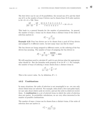
Balka ISE 1.10 6.2. PROPERTIES OF CONTINUOUS PROBABILITY DISTRIBUTIONS 143
6.2 Properties of Continuous Probability Distributions
There are a few properties common to all continuous probability distributions:
• The value of f(x) is the height of the curve at point x. The curve cannot
dip below the x axis (f(x) ≥ 0 for all x).
• The value of f(x) is not a probability, but it helps us find probabilities, since
for continuous random variables probabilities correspond to areas under
the curve. The probability that the random variable X takes on a value
between two points a and b is the area under the curve between a and b,
as illustrated in Figure 6.3.
P(a X b)
a b
x
Figure 6.3: P(a X b) is the area under the curve between a and b.
• The area under the entire curve is equal to 1. This is the continuous analog
of the discrete case, in which the probabilities sum to 1.
The next few points require a basic knowledge of integral calculus.
• Areas under the curve are found by integrating the probability density
function:
P(a X b) =
R b
a f(x)dx.
• Since the area under the entire curve must equal 1:
R ∞
−∞ f(x)dx = 1.
• The expected value of a continuous random variable is found by integration:
E(X) =
R ∞
−∞ xf(x)dx.
• The expected value of a function, g(X), of a continuous random variable
is found by integration: E[g(X)] =
R ∞
−∞ g(x)f(x)dx.
• The variance of a continuous random variable is found by integration:

V ar(X) = E[(X − µ)2] =
R ∞
−∞(x − µ)2f(x)dx.
It is often easier to calculate the variance using the relationship:
E[(X − µ)2] = E(X2) − [E(X)]2. This is a very handy relationship that is
useful in both calculations and theoretical work.
There is one more important point. The probability that a continuous random
variable X takes on any specific value is 0. (P(X = a) = 0 for all a. For example,
P(X = 3.2) = 0, and P(X = 218.28342) = 0.) This may seem strange, as the
random variable must take on some value. But probabilities are areas under a
curve, and any constant a is just a point with an infinitesimally small area above
it, so P(X = a) = 0. In a discussion of continuous random variables, we will
only discuss probabilities involving a random variable falling in an interval of
values, and not the probability that it equals a specific value. Also note that for
any constant a, P(X ≥ a) = P(X a) and P(X ≤ a) = P(X a).
6.2.1 An Example Using Integration
Optional 8msl supporting videos available for this section:
Finding Probabilities and Percentiles for a Continuous Probability Distribution (11:59) (http://youtu.be/EPm7FdajBvc)
Deriving the Mean and Variance of a Continuous Probability Distribution (7:22) (http://youtu.be/Ro7dayHU5DQ)
If you are not required to use integration, this section can be skipped. (But
taking a quick look at the plots might be informative.)
Example 6.1 Suppose the random variable X has the probability density func-
tion:
f(x) =

cx2 for 1 x 2
0 elsewhere
Q: What value of c makes this a legitimate probability distribution?
A: We need to find the value c such that
R ∞
−∞ f(x)dx = 1. In other words, we
need to find c such that the area under the entire curve is 1. (See Figure 6.4).
The resulting pdf is:
f(x) =
3
7x2 for 1 x 2
0 elsewhere
Q: What is P(X 1.5)?

Z ∞
−∞
f(x)dx = 1
=⇒
Z 2
1
cx2
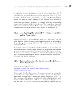
dx = 1
=⇒ c
Z 2
1
x2
dx = 1
=⇒ c[
x3
3
]2
1 = 1
=⇒ c[
8
3
−
1
3
] = 1
=⇒ c =
3
7
1 2
x
f(x) = cx2
This area must
equal 1
Figure 6.4: The area under the curve must equal 1.
P(X 1.5) =
Z 1.5
1
f(x)dx
=
Z 1.5
1
3
7
x2
dx
=
x3
7
|1.5
1
=
1.53
7
−
13
7
≈ 0.339 1.0 1.5 2.0
x
f(x) =
3
7
x2
P(X 1.5)
Figure 6.5: P(X 1.5) is the area to the left of 1.5.
A: P(X 1.5) is the area under f(x) to the left of 1.5, as illustrated in Figure 6.5.
Q: What is the 75th percentile of this distribution?
A: The 75th percentile is the value of x such that the area to the left is 0.75, as
illustrated in Figure 6.6.
Q: What is the mean of this probability distribution?
A: E(X) =
R ∞
−∞ xf(x)dx, illustrated in Figure 6.7.
There are many different continuous probability distributions that come up fre-
quently in theoretical and practical work. Two of these, the uniform distribution

Balka ISE 1.10 6.3. THE CONTINUOUS UNIFORM DISTRIBUTION 146
Let a represent the 75th per-
centile. Then:
Z a
−∞
f(x)dx = 0.75
=⇒
Z a
1
3
7
x2
dx = 0.75
=⇒
x3
7
|a
1
=⇒
a3 − 1
7
= 0.75
=⇒ a ≈ 1.842
1 2
x
f(x) =
3
7
x2
75th percentile
0.75
Figure 6.6: The 75th percentile.
E(X) =
Z ∞
−∞
xf(x)dx
=
Z 2
1
x ·
3
7
x2
dx
=
3
7
[
x4
4
]2
1
=
3
7
[
16
4
−
1
4
]
=
45
28
1.0 1.5 2.0
f(x) =
3
7
x2
E(X)
Figure 6.7: Expected value of X.
and the normal distribution, are described in the following sections.
6.3 The Continuous Uniform Distribution
Optional 8msl supporting video available for this section:
Introduction to the Continuous Uniform Distribution (7:03) (http://youtu.be/izE1dXrH5JA)
The simplest continuous distribution is the uniform distribution. For both theo-
retical and practical reasons it is an important distribution, but it also provides
a simple introduction to continuous probability distributions. For the continuous
uniform distribution, areas under the curve are represented by rectangles, so no
integration is required.

In the continuous uniform distribution, the random variable X takes on values
between a lower bound c and an upper bound d, and all intervals of equal length
are equally likely to occur. Figure 6.8 illustrates the most common continuous
uniform distribution (c = 0, d = 1). This is sometimes called the standard
uniform distribution.
0.0 0.5 1.0
0.0
0.5
1.0
1.5
x
f(x)
Figure 6.8: Uniform distribution with a lower bound of 0 and an upper bound
of 1.
The area under the entire curve must equal 1, so in this case the height of the
curve at its peak must equal 1. In the general case:
f(x) =



1
d − c
for c ≤ x ≤ d
0 elsewhere
For a continuous uniform distribution, µ = d+c
2 , and σ2 = 1
12(d − c)2.
The shape of the continuous uniform distribution will be a simple rectangle,
which makes it easy to calculate probabilities and discuss the basic concepts of
continuous probability distributions. Let’s look at a continuous uniform distri-
bution that has bounds different from 0 and 1, as this best illustrates a few
points.
Example 6.2 Suppose a continuous random variable X has the continuous uni-
form distribution with a minimum of 100 and a maximum of 150. This is illus-
trated in Figure 6.9.
The area under the entire curve is a rectangle with a base of 150 − 100 = 50,
and a height of f(x). We know that the area under the entire curve must equal
1, and we also know that the area of a rectangle is base × height. We can easily
find what the height of the curve must be: f(x) = 1
150−100 = 1
50. More formally,

80 100 125 150 170
0.00
0.01
0.02
0.03
x
f(x)
Figure 6.9: A uniform distribution with a lower bound of 100 and an upper
bound of 150.
for this distribution:
f(x) =



1
50
for 100 ≤ x ≤ 150
0 elsewhere
The random variable X can only take on values between 100 and 150. Let’s look
at a few calculations involving this distribution.
Q: What is P(X 130)?
A: Since probabilities are areas under the curve, P(X 130) is simply the area
to the right of 130, as illustrated in Figure 6.10. This area is a rectangle, with a
base of 150 − 130 = 20 and a height of f(x) = 0.02. The area to the right of 130
is P(X 130) = 20 · 0.02 = 0.40.
80 100 150 170
130
0.00
0.01
0.02
0.03
x
f(x)
P(X 130)
Figure 6.10: The probability that X takes on a value greater than 130.
Q: What is P(85 X 137.25)?
A: There is no area between 85 and 100 (P(85 X 100) = 0), and thus
P(85 X 137.25) = P(100 X 137.25)

P(100 X 137.25) is the area under the curve between 100 and 137.25,
P(100 X 137.25) = (137.25 − 100) · 0.02 = 37.25 · 0.02 = 0.745
80 100 150 170
137.25
0.00
0.01
0.02
0.03
x
f(x)
P(100 X 137.25)
Figure 6.11: The probability that X takes on a value between 100 and 137.5.
Q: What is the median of this probability distribution? Equivalently, what is
the median of the random variable X ?
A: The median is the value of the variable that splits the distribution in half (50%
of the area to the left, and 50% of the area to the right). For this distribution,
the median is 125.
Q: What is the mean of this probability distribution?
A: Finding the mean of a continuous probability distribution can be a little tricky,
as it often requires integration (E(X) =
R ∞
−∞ xf(x)dx). But it can be found for
the uniform distribution rather easily. For symmetric distributions the mean and
median are equal, and thus for this distribution, mean = median = 125.
Q: What is the 17th percentile of this distribution?
A: The 17th percentile is the value of x such that the area to the left of x is 0.17.
If we let a represent the 17th percentile, then by the definition of a percentile
the area to the left of a is 0.17, as illustrated in Figure 6.12. We also know that
the area to the left of a is the area of a rectangle with a base of (a − 100) and a
height of 0.02. So the area to the left of a is: base × height = (a − 100) · 0.02.
Combining these two pieces of information, we know that (a − 100) · 0.02 must
equal 0.17. This implies that a = 108.5, and thus the 17th percentile of this
distribution is 108.5.

Balka ISE 1.10 6.4. THE NORMAL DISTRIBUTION 150
80 100 150 170
0.00
0.01
0.02
0.03
x
f(x)
17th percentile
.17
Figure 6.12: 17th percentile for this uniform distribution.
The calculations for the continuous uniform distribution are straightforward, but
other continuous distributions have more complicated density functions. Find-
ing the area under these curves involves integrating the density function, which
sometimes requires numerical techniques. Finding areas under these distributions
often involves using statistical software, or looking up the appropriate values in
a table.
6.4 The Normal Distribution
An Introduction to the Normal Distribution (5:27) (http://youtu.be/iYiOVISWXS4)
The normal distribution2 is an extremely important continuous probability dis-
tribution. Many variables have distributions that are approximately normal, and
many statistical inference techniques are based on the normal distribution. The
normal distribution is sometimes called bell-shaped, as it resembles the profile of
a bell. Figure 6.13 illustrates a normal distribution with µ = 33.1 and σ = 2.1,
which is (approximately) the distribution of the total amount of fat in 100 grams
of cheddar cheese.3
The probability density function (pdf) of the normal distribution is:
f(x) =
1
√
2πσ
e− 1
2σ2 (x−µ)2
2
The normal distribution is often called the Gaussian distribution, in honour of Carl Friedrich
Gauss.
3
U.S. Department of Agriculture, Agricultural Research Service. 2013. USDA National Nu-
trient Database for Standard Reference, Release 26. Nutrient Data Laboratory Home Page,
http://www.ars.usda.gov/ba/bhnrc/ndl.

0.00
0.05
0.10
0.15
0.20
25 30 35 40 45
f(x)
Total Fat (x)
33.1
Figure 6.13: The distribution of the total amount of fat, in grams, in 100 grams
of cheddar cheese. (A normal distribution with µ = 33.1 and σ = 2.1.)
If a random variable X has the normal distribution, then it can take on any finite
value x: −∞ x ∞.4
The normal distribution has two parameters: µ and σ. The normal distribution
is symmetric about µ (see Figure 6.14a). µ is both the mean and median of the
distribution, and it can be any finite value: −∞ µ ∞.
Once again, σ represents the standard deviation of the probability distribution.
As illustrated in Figure 6.14, 68.3% of the area under the normal curve lies
within 1 standard deviation of the mean, 95.4% of the area lies within 2 standard
deviations of the mean, and 99.7% of the area lies within 3 standard deviations
of the mean.5 (We’ll learn how to find these areas in Section 6.4.1.)
The greater the standard deviation, the more spread out the distribution and
the lower the peak. Figure 6.15 shows two different normal distributions. The
two distributions have equal means but different standard deviations.
There are an infinite number of normal distributions—sometimes called a family
of normal distributions—corresponding to different values of µ and σ. If the
random variable X has a normal distribution with mean µ and variance σ2, we
write this as X ∼ N(µ, σ2).6
The standard normal distribution is a normal distribution with µ = 0 and
4
This may seem to be a problem for modelling variables that take on only positive values (total
grams of fat, for example), but it is not a problem in practice. There will always be some
positive probability that X 0 for a normally distributed random variable, but depending on
the parameters of the distribution it can be very, very, very close to 0.
5
The empirical rule, discussed in Section 3.3.3.1, is based on the normal distribution.
6
Some sources put the standard deviation (not the variance) as the second term in the paren-
theses: X ∼ N(µ, σ), so be careful if you are looking at different sources!

µ
(a) The normal distribution is symmetric
about µ.
µ µ + σ
µ − σ
0.683
(b) 68.3% of the area lies within 1 standard
deviation of the mean.
µ µ + 2σ
µ − 2σ
0.954
(c) 95.4% of the area lies within 2 standard
deviations of the mean.
µ µ + 3σ
µ − 3σ
0.997
(d) 99.7% of the area lies within 3 standard
deviations of the mean.
Figure 6.14: Illustration of µ and σ for the normal distribution.
µ
σ1
σ2 = 2σ1
Figure 6.15: Two normal distributions. The standard deviation of the distribu-
tion in red is double the standard deviation of the distribution in black.
σ = 1. We often represent standard normal random variables with the letter
Z (Symbolically, Z ∼ N(0, 1).) Figure 6.16 illustrates the standard normal
distribution.
Finding areas and percentiles for the normal distribution requires integrating the
probability density function. Unfortunately, there is no closed form solution and
the curve must be integrated numerically. Fortunately, any statistical software

-4 -3 -2 -1 0 1 2 3 4
Figure 6.16: The standard normal distribution.
will have a function that yields areas under the normal curve. We will find areas
and percentiles for the normal distribution using software, or by using tabulated
values for the standard normal distribution.
6.4.1 Finding Areas Under the Standard Normal Curve
At various points throughout the remainder of this text we will need to find
areas under the standard normal curve. We will find these areas using software
or a standard normal table. Our standard normal table gives the cumulative
distribution function of the standard normal distribution. In other words, if we
look up a value z in the table, the table yields F(z), the area to the left of z
under the standard normal curve, as illustrated in Figure 6.17.7
We can use the area to the left to find any area that we require. We need only
the important information that the area under the entire curve equals 1. It is
also useful to note that the standard normal distribution is symmetric about 0.
Let’s look at a few examples.
Q: What is P(Z 1.71)?
A: When faced with these problems, it is a good idea to first draw a quick sketch
of the standard normal distribution and shade the required area. The appropriate
plot is given in Figure 6.18a. Our standard normal table gives the area to the left
of the z value, so to find this area we look up 1.71 in the table (see Figure 6.18b).
The value in the table is our answer: P(Z 1.71) = 0.9564. We can also find
7
There are different table formats. This one is chosen because students find it easiest to use,
and it is consistent with the output from software. Be careful if you are looking up tables
online, as the table may be set up a little differently.

0 z
The table gives this area
Figure 6.17: Areas in the table.
this area using software (Figure 6.18c gives the R code that yields the area to
the left of 1.71). When possible, it is better to use software than the table.
0.9564
0 1.71
(a) The area we need to find.
(b) Finding the area using the standard normal table. (c) Finding the area using R.
Figure 6.18: The area to the left of 1.71 under the standard normal curve.
Q: What is P(Z 1.71)?
A: We should draw a picture, shading the area that we require. The required
area is illustrated in Figure 6.19.

0.9564
1 − 0.9564
0 1.71
Figure 6.19: P(Z 1.71)
Here we need the area to the right of 1.71. The table gives the area to the left
of 1.71. Since the area under the entire curve is 1, P(Z 1.71) = 1 − P(Z
1.71) = 1 − 0.9564 = 0.0436.
Verify the following probabilities using similar logic to that used above.
P(1.23 Z 2.27) = P(Z 2.27) − P(Z 1.23) = 0.9884 − 0.8907 = 0.0977
P(−2.00 Z 2.00) = P(Z 2) − P(Z −2) = 0.9772 − 0.0228 = 0.9544
In many situations we will need to find percentiles of the standard normal dis-
tribution. For example, we may need to find the value of z such that the area
to the left is 0.99. In the following questions we need to find percentiles (we are
given a probability, and we need to find the value z that makes the statement
true).
Q: Find the value z such that the area to the right is 0.1788.
A: It is best to illustrate the scenario with a plot, as in Figure 6.20. We cannot
.1788
The table gives this area
z
0
Figure 6.20: Table area when area to the right of z is 0.1788.

simply run off to the table and look up 0.1788. This is not how the table is set up;
our table gives the area to the left of z. If the area to the right of z is 0.1788, this
implies the area to the left of z is 1 − 0.1788 = 0.8212. If we look into the body
of the standard normal table and find 0.8212, we will see that the corresponding
value of z is 0.92 (see Figure 6.21b). This means that P(Z 0.92) = 0.8212 and
P(Z 0.92) = 0.1788, and thus the answer to the question is 0.92. We can also
find this z value using software (Figure 6.21c shows the R command that yields
the appropriate z value).
0
0.92
0.1788
0.8212
(a) We need to find the z value that yields an area to
the left of 0.8212.
(b) Finding the z value using the table. (c) Finding the z value with R.
Figure 6.21: Finding the z value with an area to the right of 0.1788.
Q: Find the 95th percentile of the standard normal distribution.
A: By the definition of a percentile, this is equivalent to finding the value of z
such that the area to the left is 0.95. The appropriate value of z is illustrated in
Figure 6.22.
If we look up 0.95 in the body of the table, we find that the two closest values are
0.9495 and 0.9505. These correspond to z values of 1.64 and 1.65, implying the
95th percentile of the standard normal distribution lies between 1.64 and 1.65.
Using software, we can find the correct value to 3 decimal places is 1.645.8
8
Under most circumstances, picking the nearest value in the table is good enough. There is
no need to average or linearly interpolate—if we need to be precise we should use software.

This area is 0.95
0
95th percentile
Figure 6.22: The 95th percentile of the standard normal distribution.
Q: Find the 5th percentile of the standard normal distribution.
A: Using a similar argument to the previous question, we can find from the table
that the 5th percentile is −1.645. We could also have used an argument based on
the symmetry of the normal distribution: Since the standard normal distribution
is symmetric about 0, the 5th percentile will have the same magnitude as the
95th percentile, but it will be negative. Thus, the 5th percentile is −1.645.
The notation za is often used to represent the value of a standard normal random
variable that has an area of a to the right. For example:
• z.05 = 1.645 (see Figure 6.23). The area to the right of 1.645 under the
standard normal curve is .05.
• z.95 = −1.645. The area to the right of −1.645 is .95.
z0.05
0.05
Figure 6.23: A commonly used notation (here z0.05 = 1.645).
It is strongly recommended that you work through the examples of this section
until you understand them and can do them perfectly. It is also strongly recom-
But the 95th percentile is an important number that comes up frequently, so we should get it
right.

mended that you always draw a picture, illustrating the problem at hand, before
running off to a table or software.
6.4.2 Standardizing Normally Distributed Random Variables
Standardizing Normally Distributed Random Variables (10:28)
(http://youtu.be/4R8xm19DmPM)
Suppose a random variable X is normally distributed with mean µ and standard
deviation σ. We can convert X into a random variable having the standard
normal distribution, allowing us to use the standard normal distribution for
probability calculations. If we let
Z =
X − µ
σ
then Z is a random variable having the standard normal distribution. Symbol-
ically, Z ∼ N(0, 1). Using this linear transformation, any normally distributed
random variable can be converted into a random variable that has the standard
normal distribution.
Example 6.3 Parents often want to know if their child’s growth is progressing
in a typical fashion. One characteristic of the size of a child is the length of their
upper arm. A study9 showed that the length of the upper arm in one-year-old
American girls is approximately normally distributed with a mean of 16.1 cm
and a standard deviation of 1.3 cm, as illustrated in Figure 6.24.
10 12 14 16 18 20 22
Upper Arm Length (cm)
Figure 6.24: The (approximate) distribution of upper arm length in one-year-old
American girls.
Q: What is the probability that a randomly selected one-year-old American girl
has an upper arm length less than 18.0 cm?
9
Fryar et al. (2012). Anthropometric reference data for children and adults: United states,
2007–2010. National Center for Health Statistics. Vital Health Stat., 11(252).

A: Let X represent the length of the upper arm. Then X is approximately
normally distributed with µ = 16.1 and σ = 1.3. In symbols, X ∼ N(16.1, 1.32).
P(X 18.0) = P(
X − µ
σ

18.0 − µ
σ
)
= P(Z
18.0 − 16.1
1.3
)
= P(Z 1.462)
= 0.928
(See Figure 6.25.)
10 12 14 16 18 20 22
Upper Arm Length (cm)
0.928
-4 -2 0 2 4
1.462
0.928
z
Figure 6.25: The area to the left of 18.0 under the distribution of upper arm
length is the same as the area to the left of 1.462 under the standard normal
curve.
Q: What is the 20th percentile of the upper arm length of one-year-old American
girls?
A: Here we need to:
1. Find the 20th percentile of the standard normal distribution.
2. Convert from Z to X. We know that Z =
X − µ
σ
, which implies X = µ+σZ.

From software or a standard normal table we can find that the 20th percentile
of the standard normal distribution is approximately −0.84. The 20th percentile
of arm length is thus: µ + σz = 16.1 + 1.3(−0.84) = 15.01 cm (see Figure 6.26.)
10 12 14 16 18 20 22
Upper Arm Length
20th percentile
(15.01)
0.20
-4 -2 0 2 4
0.20
z
20th percentile
(-0.84)
Figure 6.26: The 20th percentile of the standard normal distribution and the
20th percentile of the distribution of upper arm length.
Example 6.4 According to some sources, the length of human pregnancies has
an approximately normal distribution with a mean of 266 days, and a standard
deviation of 16 days.
Q: For a randomly selected pregnant woman, what is the probability that the
pregnancy lasts less than 238.0 days?
A: Let X be a random variable representing pregnancy length. X is distributed
approximately normally with a mean of µ = 266 and a standard deviation of
σ = 16.
P(X 238.0) = P(
X − µ
σ

238.0 − µ
σ
)
= P(Z
238.0 − 266
16
)
= P(Z −1.75)
= 0.0401

(See Figure 6.27).
0.0401
-1.75 0
Figure 6.27: The probability the pregnancy lasts less than 238.0 days.
Q: For a randomly selected pregnant woman, what is the probability that the
pregnancy lasts longer than 270.0 days?
A:
P(X 270.0) = P(Z
270.0 − 266
16
) = P(Z 0.25) = 1 − 0.5987 = 0.4013
Q: What is the 75th percentile of pregnancy length?
A: Figure 6.28 illustrates the 75th percentile of the distribution of pregnancy
lengths.
75th percentile
This area is 0.75
266
Figure 6.28: 75th percentile of pregnancy length.
Using software or a standard normal table, we can find that the 75th percentile of
the standard normal distribution is approximately 0.67. Since z = x−µ
σ , and thus

Balka ISE 1.10 6.5. NORMAL QUANTILE-QUANTILE PLOTS 162
x = µ + σz, the 75th percentile of human pregnancy lengths is approximately
266 + 16 · 0.67 = 276.7 days.
Example 6.5 Scores on a certain IQ test are approximately normally distributed
with a mean of 100.0, and a standard deviation of 14.5.
Q: If a randomly picked person takes the test, what is the probability they score
less than 130?
A: X is approximately normally distributed with a mean of 100, and a standard
deviation of 14.5, and thus:
P(X 130) = P(Z
130 − 100
14.5
) = P(Z 2.07) = 0.981
Q: What is the lowest score that would put a person in the top 5% of the
population?
A: This is equivalent to asking for the 95th percentile of scores on the test. We
need to find the 95th percentile of the standard normal, then convert back to X.
Using software or a standard normal table, we can find that the 95th percentile
of the standard normal is approximately 1.645. The 95th percentile of the IQ
scores is thus µ + σz = 100 + 14.5 · 1.645 = 123.85.
6.5 Normal Quantile-Quantile Plots: Is the Data Ap-
proximately Normally Distributed?
Normal Quantile-Quantile Plots (12:09) (http://youtu.be/X9_ISJ0YpGw)
The inference procedures encountered later in this text often require the as-
sumption of a normally distributed population. These inference procedures can
break down and perform poorly if the normality assumption is not true, so this
assumption should always be investigated.
In practice we will never know for certain whether a population is normally
distributed, but if the sample is approximately normal, that gives some indication
that the population may be approximately normal. To investigate normality in
the sample, we could plot a frequency histogram, but this is not as informative
as a normal quantile-quantile (QQ) plot. There are several different techniques
and plotting methods, but in all cases we end up with an approximately straight

line if the data is approximately normally distributed. Figure 6.29 illustrates a
normal quantile-quantile plot for a random sample of 50 values from a normally
distributed population.
-2 -1 0 1 2
-1.5
-1.0
-0.5
0.0
0.5
1.0
1.5
Theoretical Quantiles
Sample
Quantiles
Figure 6.29: Normal QQ plot for a random sample of 50 values from a normally
In a normal quantile-quantile plot the ordered data values from the sample are
plotted against the appropriate quantiles of the standard normal distribution.10
If the sample data is approximately normally distributed, this technique will re-
sult in points that lie on an approximately straight line. If the plot shows system-
atic deviations from linearity (curvature, for example) then this gives evidence
that the population is not normally distributed—inference procedures based on
the normal distribution may not be appropriate.
Normal QQ plots are typically carried out using software, so for us the calcula-
tions are not as important as properly interpreting the resulting plot.
6.5.1 Examples of Normal QQ Plots for Different
Distributions
Properly interpreting a normal QQ plot is difficult without some experience.
Let’s look at a few plots to get some perspective on what normal quantile-quantile
plots look like under normality and for some other distributions.
Figure 6.30 shows a normal distribution and normal quantile-quantile plots for 3
random samples of size 50 from a normal distribution. Note that there is some
variability from sample to sample, but overall the points fall close to a straight
line.
10
This can be carried out in a variety of related ways. The basic idea is that each ordered data
value from the sample is plotted against the value we would expect to get if the data were
normally distributed. One possibility is to plot the ith ordered data value against the value
of z that has an area of i
n+1
to the left, under the standard normal curve. You can see some
alternative possibilities in the Wikipedia article: http://en.wikipedia.org/wiki/Q-Q_plot

Figure 6.31 illustrates a uniform distribution and normal quantile-quantile plots
for 3 random samples of size 50 from a uniform distribution. Note the curvature
in the tails of the normal QQ plot—the tails of the uniform distribution are
truncated, and shorter relative to the normal distribution,
Figure 6.32 shows an exponential distribution and normal quantile-quantile plots
for 3 random samples of size 50 from an exponential distribution. Note the cur-
vature in the normal QQ plots—curvature of this type indicates right skewness.
There are a variety of other deviations from normality that are encountered, such
as extreme outliers and tails that are heavier than normal.
Normal quantile-quantile plots will be encountered at various points for the re-
mainder of this text.
0
x
f(x)
Sample
Quantiles
(b) Normal QQ plot for a random sam-
ple.
Sample
Quantiles
(c) Normal QQ plot for a random sam-
ple.
Sample
Quantiles
(d) Normal QQ plot for a random sam-
ple.
Figure 6.30: Normal QQ plots for 3 random samples of size 50 from a normally

0
x
f(x)
(a) A uniform distribution.
Sample
Quantiles
(b) Normal QQ plot.
Sample
Quantiles
(c) Normal QQ plot.
Sample
Quantiles
(d) Normal QQ plot.
Figure 6.31: Normal QQ plots for 3 random samples of size 50 from a uniformly
0
x
f(x)
(a) An exponential distribution.
Sample
Quantiles
(b) Normal QQ plot.
Sample
Quantiles
(c) Normal QQ plot.
Sample
Quantiles
(d) Normal QQ plot.
Figure 6.32: Normal QQ plots for 3 random samples of size 50 from an exponen-
tial distribution.

Balka ISE 1.10 6.6. OTHER IMPORTANT CONTINUOUS PROBABILITY DISTRIBUTIONS 166
6.6 Other Important Continuous Probability Distri-
butions
There are several other continuous probability distributions that are frequently
encountered in statistical inference. Here three distributions are introduced:
the χ2 distribution, the t distribution, and the F distribution. All three are
related to the normal distribution, and arise when we are sampling from normally
distributed populations in different situations. We will use all 3 distributions later
in this text.
6.6.1 The χ2
Distribution
An Introduction to the Chi-Square Distribution (5:29) (http://youtu.be/hcDb12fsbBU)
The χ2 distribution11 is related to the standard normal distribution. If the
random variable Z has the standard normal distribution, then Z2 has the χ2
distribution with one degree of freedom. These distributions are illustrated in
Figure 6.33.
-4 -2 0 2 4
z
(a) The distribution of Z.
0 1 2 3 4 5 6
z2
(b) The distribution of Z2
.
Figure 6.33: The standard normal distribution and the χ2 distribution with 1
degree of freedom.
Also, the sum of squared independent standard normal random variables has a χ2
distribution. More formally, if Z1, Z2, . . . , Zk are independent standard normal
random variables, then Z2
1 +Z2
2 +. . .+Z2
k has the χ2 distribution with k degrees of
freedom. For example, if we add 3 squared independent standard normal random
variables, their sum has a χ2 distribution with 3 degrees of freedom. The pdf of
the χ2 distribution with k degrees of freedom is:
11
The symbol χ is the lowercase Greek letter chi (rhymes with sky). Read “χ2
” as “chi-square”.

f(x) =
(
xk/2−1e−x/2
2k/2Γ(k/2)
for x ≥ 0
0 otherwise
Where Γ represents the gamma function.12 This pdf might look intimidating,
but as with the normal distribution we will not be working with it directly. (We
will use software or tables to find areas and percentiles.) Figure 6.34 illustrates
the χ2 distribution for various degrees of freedom.
0
0 5 10 15 20 25
χ2
Density
3 DF
6 DF
12 DF
Figure 6.34: Three χ2 distributions.
A few points to note:
• The χ2 distribution has a minimum of 0.
• The distribution is skewed to the right. The skewness decreases as the
degrees of freedom increase.
• A χ2 distribution with k degrees of freedom has a mean of k and a variance
of 2k. Note that the mean increases as the degrees of freedom increase.
• For k ≥ 2, the mode of the χ2 distribution occurs at k − 2. For k ≤ 2 the
mode occurs at 0.
• Areas under the curve can be found using software or a χ2 table.
We will use the χ2 distribution in Section 12.3 when we discuss inference pro-
cedures for a single variance, and in Chapter 13, when we discuss χ2 tests for
count data.
12
For integer a, Γ(a) = (a − 1)!. In the general case, Γ(a) =
R ∞
0
e−t
ta−1
dt.

6.6.2 The t Distribution
An Introduction to the t Distribution (6:10) (http://youtu.be/T0xRanwAIiI)
The t distribution is a continuous probability distribution that arises in a vari-
ety of different statistical inference scenarios. The t distribution is often called
Student’s t distribution.13
The t distribution is strongly related to the standard normal distribution. Sup-
pose Z is a standard normal random variable, U is a χ2 random variable with ν
degrees of freedom, and Z and U are independent. Then:
T =
Z
p
U/ν
has the t distribution with ν degrees of freedom. The probability density function
of the t distribution is:
f(x) =
Γ(ν+1
2 )
√
νπΓ(ν
2 )
(1 +
x2
ν
)−ν+1
2 for −∞ x ∞
The t distribution has a single parameter, the degrees of freedom ν. The degrees
of freedom ν must be greater than 0, and in practical situations ν is typically a
positive integer.
We will not be working with the t distribution pdf directly, as we will use software
or a t table to find areas and percentiles.
The shape of the t distribution depends on the degrees of freedom ν. It has a
similar appearance to the standard normal distribution, but with heavier tails
and a lower peak, as illustrated in Figure 6.35.
• The t distribution has a median of 0 and is symmetric about 0.
• The mean of the t distribution is 0 (for ν 1).
• The variance of the t distribution is ν
ν−2 (for ν 2). Note that the variance
of the t distribution is greater than that of the standard normal distribu-
tion.
13
In honour of William Gosset, who played a fundamental role in its development, and who
published under the pseudonym Student.

-6 -4 -2 0 2 4 6
Standard Normal
t with 2 df
t with 4 df
Figure 6.35: The standard normal distribution, a t distribution with 2 degrees
of freedom, and a t distribution with 4 degrees of freedom.
• As the degrees of freedom increase, the t distribution tends toward the
standard normal distribution. A t distribution with infinite degrees of
freedom is equivalent to the standard normal distribution.
• Areas under the curve and percentiles can be found using software or a t
table.
The t distribution is very commonly used in statistical inference. It often arises in
statistical inference on means when we are sampling from a normally distributed
population. We will use the t distribution in several places in the text, beginning
in Section 8.3.
6.6.3 The F Distribution
An Introduction to the F Distribution (4:04) (http://youtu.be/G_RDxAZJ-ug)
The F distribution14 is another important continuous probability distribution
that is widely used in statistical inference. The F distribution is related to the
χ2 distribution. If we let the random variable U1 have the χ2 distribution with ν1
degrees of freedom, and we let the random variable U2 have the χ2 distribution
with ν2 degrees of freedom, and U1 and U2 are independent, then:15
F =
U1/ν1
U2/ν2
14
The F distribution was so named in honour of R.A. Fisher, the “father of modern statistics”.
15
In words, the F distribution arises as the distribution of the ratio of two independent χ2
random variables, divided by their respective degrees of freedom.

has the F distribution with ν1 degrees of freedom in the numerator, and ν2
degrees of freedom in the denominator.
An important implication of this is that the F distribution often arises when
we are working with ratios of variances. We will encounter this in Section 12.4
(Inference for Two Variances) and Chapter 14 (Analysis of Variance).
The pdf of the F distribution with ν1 and ν2 degrees of freedom:
f(x) =





Γ(
ν1+ν2
2
)(
ν1
ν2
)
ν1
2 x
ν1
2 −1
Γ(
ν1
2
)Γ(
ν2
2
)(1+
ν1
ν2
x)
ν1+ν2
2
for x ≥ 0
0 otherwise
As with the normal, t, and χ2 distributions, we will not be working with this pdf
directly. (We will use software or tables to find areas and percentiles for the F
distribution.)
The shape of the F distribution depends on the degrees of freedom. Figure 6.36
illustrates the F distribution for a few different sets of degrees of freedom.
0 1 2 3 4 5 6
Density
F
3 and 8 DF
8 and 3 DF
20 and 20 DF
Figure 6.36: Three F distributions.
• The F distribution has a minimum of 0.
• The F distribution has some right skewness (the extent of the skewness
depends on the degrees of freedom), as seen in Figure 6.36.
• An F distribution with ν1 degrees of freedom in the numerator and ν2
degrees of freedom in the denominator has a mean of µ = ν2
ν2−2 (provided
ν2 2).

• If ν1 = ν2, then the median is exactly 1. If ν1 6= ν2, then the median will
not be exactly 1, but it is often (roughly speaking) in the neighbourhood
of 1.
• Areas under the curve and percentiles can be found using software or an
F table.

6.7 Chapter Summary
A continuous random variable can take on an infinite number of possible values,
corresponding to all values in an interval. We model continuous random variable
with a curve, f(x), called a probability density function (pdf). The pdf helps us
find probabilities, since for continuous random variables probabilities are areas
under the curve. The probability that the random variable X lies between two
points a and b is the area under the curve between a and b: P(a X b) =
R b
a f(x)dx. The area under the entire curve is equal to one (
R ∞
−∞ f(x)dx = 1).
The simplest continuous probability distribution is the continuous uniform dis-
tribution, in which f(x) is constant over the range of x. For this distribution,
probability calculations are simple as we only need to find the areas of rectangles.
The normal distribution is an extremely important continuous probability dis-
tribution. Its pdf: f(x) = 1
√
2πσ
e− 1
2σ2 (x−µ)2
. This distribution is “bell shaped”,
0
x
f(x)
Figure 6.37: A normal distribution.
If a random variable X has the normal distribution, then it can take on any finite
value: −∞ x ∞
The normal distribution has two parameters, µ (the mean) and σ (the standard
deviation). Since the normal distribution is symmetric, the mean and median are
equal: Mean = Median = µ. The mean can be any finite value (−∞ µ ∞),
but the standard deviation must be positive (σ 0).
The standard normal distribution is a normal distribution with a mean of 0 and
a standard deviation of 1. Areas under the standard normal curve can be found
using an appropriate table or statistical software.
Suppose a random variable X is normally distributed with mean µ and and stan-
dard deviation σ. If we use the linear transformation:
Z =
X − µ
σ

then Z is a random variable having the standard normal distribution.
In a normal quantile-quantile plot, the observations are plotted in such a way
that the points fall on an approximately straight line if the data is approximately
normally distributed. This can help to determine whether it is reasonable to
think that a population is approximately normally distributed. This is important
because many of the inference procedures used later in the text assume a normally
The χ2, t, and F distributions are important continuous probability distributions
that were introduced in this chapter and will be used later in this text.

Chapter 7
Sampling Distributions
175

Balka ISE 1.10 176
• Sampling Distributions: Introduction to the Concept (7:52)
(http://youtu.be/Zbw-YvELsaM)
• The Sampling Distribution of the Sample Mean (11:40) (http://youtu.be/q50GpTdFYyI)
• Introduction to the Central Limit Theorem (13:14) (http://youtu.be/Pujol1yC1_A)
• Deriving the Mean and Variance of the Sample Mean (5:07)
(http://youtu.be/7mYDHbrLEQo)
• Proof that the Sample Variance is an Unbiased Estimator of the Population
Variance (6:58)
(http://youtu.be/D1hgiAla3KI)

7.1 Introduction
Sampling Distributions: Introduction to the Concept (7:52) (http://youtu.be/Zbw-YvELsaM)
The concept of the sampling distribution of a statistic is fundamental to much
of statistical inference. Properly interpreting the results of a statistical inference
procedure is much easier when one has a solid understanding of this important
topic. This chapter provides an introduction to sampling distributions, and the
sampling distribution of the sample mean is discussed in detail.
Recall that the population is the entire group of individuals or items that we
want information about, and the sample is the subset of the population that
we actually examine. We will soon use sample statistics to estimate and make
inferences about population parameters. For example, the sample mean X̄ is an
estimator of the population mean µ. We would like to know how close the value
of X̄ is to µ, but in most situations it is impossible to know the precise value
of the difference (since we do not typically know the value of parameters). How
will we measure how close the estimate is likely to be to the parameter? We use
arguments based on the sampling distribution of the statistic.
The sampling distribution of a statistic is the probability distribution of that
statistic (the distribution of the statistic in all possible samples of the same size).
This is often phrased in terms of repeated sampling: the sampling distribution of
a statistic is the probability distribution of that statistic if samples of the same
size were to be repeatedly drawn from the population.
Example 7.1 A professor thinks that they could prepare more appropriate
course materials if they knew the average age of the 16 students in their class.
The 16 students represent the entire population of interest to the professor, since
the professor is trying to produce better materials for these specific 16 students.1
The view from the professor’s perspective and the underlying reality of the situ-
ation are illustrated in Figure 7.1.
The professor asks the university for the students’ ages. The university is wary
of violating a privacy policy, and agrees only to supply the sample mean age of
3 randomly selected students from the class. The value of the sample mean will
depend on the students that are randomly selected. If we were to repeatedly
sample 3 students from the population, the value of the sample mean would vary
from sample to sample. This is illustrated in Figure 7.2.
The sample mean X̄ is a random variable, and like all random variables it has
a probability distribution. We can investigate the distribution of the sample
1
Populations are usually much larger than this in practice, and are often infinite.

234 241 233 227
251 227 242 239
241 238 230 246
231 243 238 276
1 2 3 4
5 6 7 8
9 10 11 12
13 14 15 16
(a) From the professor’s viewpoint: 16 students
with unknown ages.
234 241 233 227
251 227 242 239
241 238 230 246
231 243 238 276
(b) The ages, in months, of the students. This
underlying reality is unknown to the professor.
Figure 7.1: The professor’s viewpoint and the reality of the situation. The
population of 16 students has a mean of µ = 239.8 months, but this is not
known to the professor.
mean by drawing many samples of size 3, calculating the sample mean for each
sample, and plotting the resulting means in a histogram. A histogram of 100,000
sample means is illustrated in Figure 7.3. This histogram is (approximately)
the sampling distribution of the sample mean2. The sample mean is distributed
about the true value of the population mean.
234 241 233 227
251 227 242 239
241 238 230 246
231 243 238 276
1 2 3 4
5 6 7 8
9 10 11 12
13 14 15 16
233
227
238
(a) Individuals 3, 6, and 15 were selected in this
sample. x̄ = 232.67.
234 241 233 227
251 227 242 239
241 238 230 246
231 243 238 276
1 2 3 4
5 6 7 8
9 10 11 12
13 14 15 16
251
238 276
(b) Individuals 5, 15, and 16 were selected in this
sample. x̄ = 255.0.
Figure 7.2: Two random samples of size 3. These samples have sample means of
232.67 and 255.0.
It is important to note that repeated sampling is an underlying concept, and
not something that we actually carry out in practice. In practice we will draw
a single sample of size n, and the statistic will take on a single value. The
2
This example involved a finite population, and so we could determine the exact sampling
distribution of X̄ by calculating the sample mean for each of the 16
3

= 560 possible sam-
ples of size 3. But the histogram of sample means in Figure 7.3 very closely resembles the
exact sampling distribution, and we often use the repeated sampling argument in statistical
inference.

230 240 250 260
0.00
0.02
0.04
0.06
0.08 Values of the Sample Mean
Relative
Frequency
µ
(239.8)
Figure 7.3: A relative frequency histogram of 100,000 sample means for Exam-
ple 7.1. This is (approximately) the sampling distribution of the sample mean
for n = 3.
value of the statistic that we see in a sample is a single value sampled from that
statistic’s sampling distribution. Mathematical arguments based on the sampling
distribution will allow us to make statements like: “We can be 95% confident
that the population mean age of students in this class lies between 219 and 246
months.”
All statistics have sampling distributions. In many situations we can determine
a statistic’s sampling distribution using mathematical arguments, instead of ac-
tually sampling repeatedly. For example, if we are randomly sampling values
from a normally distributed population, the sampling distribution of X̄ and S2
can be mathematically derived. Figure 7.4 illustrates the sampling distributions
of X̄ and S2 if we are sampling 10 values from a normally distributed population
with µ = 50 and σ2 = 4.
47 48 49 50 51 52 53
Values of the Sample Mean
µ
(a) The sampling distribution of X̄.
0 2 4 6 8 10 12 14
Values of the Sample Variance
σ2
(b) The sampling distribution of S2
.
Figure 7.4: The sampling distribution of the sample mean and sample variance
if we are sampling 10 values from a normally distributed population with µ = 50
and σ2 = 4. A statistic will vary about the value of the parameter it estimates.

Balka ISE 1.10 7.2. THE SAMPLING DISTRIBUTION OF THE SAMPLE MEAN 180
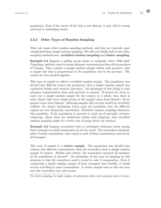
The remainder of this chapter will focus on the sampling distribution of the
sample mean. We will discuss the sampling distribution of the sample variance
and other statistics later on.
7.2 The Sampling Distribution of the Sample Mean
The Sampling Distribution of the Sample Mean (11:40) (http://youtu.be/q50GpTdFYyI)
In this section we will investigate properties of the sampling distribution of the
sample mean, including its mean (µX̄), its standard deviation (σX̄), and its
shape. It is assumed here that the population is infinite (or at least very large
compared to the sample size). This is almost always the case in practice. Slight
adjustments need to be made if we are sampling a large proportion of a finite
population.
Let X1, X2, . . . , Xn be n independently drawn observations from a population
with mean µ and standard deviation σ. Let X̄ be the sample mean of these n
independent observations: X̄ = X1+X2+...+Xn
n . Then:
• µX̄ = µ. (The mean of the sampling distribution of X̄ is equal to the mean
of the distribution from which we are sampling.)
• σX̄ =
σ
√
n
. (The standard deviation of the sampling distribution of X̄
is equal to the standard deviation of the distribution from which we are
sampling, divided by the square root of the sample size.)
• If the distribution from which we are sampling is normal, the sampling
distribution of X̄ is normal.
We can show that µX̄ = µ using the properties of expectation discussed in
Section 5.3.1.2:
E(X̄) = E(
X1 + X2 + . . . + Xn
n
)
=
1
n
E(X1 + X2 + . . . + Xn)
=
1
n
[E(X1) + E(X2) + . . . + E(Xn)]
=
1
n
nµ = µ

It can also be shown that σX̄ =
σ
√
n
, using properties of the variance:
Var(X̄) = Var(
X1 + X2 + . . . + Xn
n
)
=
1
n2
Var(X1 + X2 + . . . + Xn)
=
1
n2
[Var(X1) + Var(X2) + . . . + Var(Xn)]
=
1
n2
nσ2
=
σ2
n
and thus σX̄ =
p
Var(X̄) =
r
σ2
n
=
σ
√
n
.
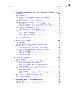
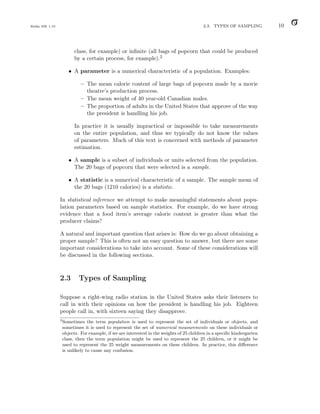
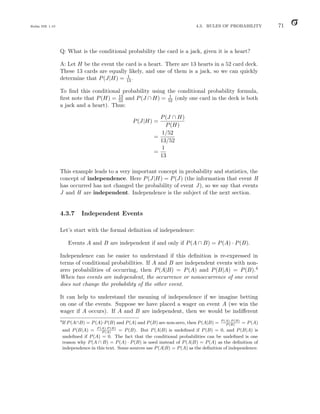
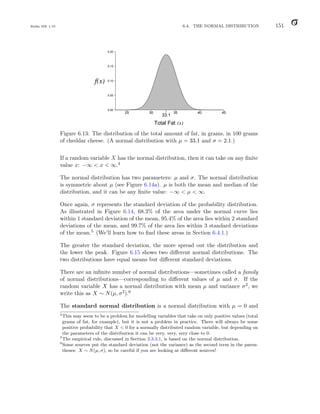
Figure 7.5 illustrates the sampling distribution of X̄ for n = 2 and n = 8 when
we are sampling from a normally distributed population with µ = 0 and σ = 10.
-40 -20 0 20 40
0.00
0.05
0.10
x
Density
n = 1
n = 2
n = 8
Figure 7.5: The sampling distribution of X̄ for n = 2 and n = 8 if we are
sampling from a normally distributed population with µ = 0 and σ = 10.
Sometimes we will need to find the probability that the sample mean falls within
a range of values. If the sample mean is normally distributed, the methods
are similar to those discussed in Section 6.4.2. But we need to take into account
that the standard deviation of the sampling distribution of X̄ is σX̄ = σ
√
n
. When
standardizing:
• As discussed in Section 6.4.2, if X is normally distributed with mean µ and
standard deviation σ, then Z = X−µ
σ has the standard normal distribution.
We will use this to find probabilities relating to a single observation.
• If X̄ is normally distributed with mean µX̄ and standard deviation σX̄ =

σ
√
n
, then Z =
X̄−µX̄
σX̄
= X̄−µ
σ/
√
n
has the standard normal distribution. We
will use this to find probabilities relating to the mean of n observations.
Example 7.2 It is well known that fast food tends to be high in sodium. The
online nutrition information at a famous fast food chain states that one of their
burgers contains 980 mg of sodium.3 There is of course some variability in the
amount of sodium in burgers of this type. Suppose that the amount of sodium
in these burgers is approximately normally distributed with a mean of 980 mg
and a standard deviation of 50 mg.4
Q: If a single burger of this type is randomly selected, what is the probability it
contains more than 1000 mg of sodium?
A: Since we are interested in a probability relating to a single observation, we
will standardize using Z =
X − µ
σ
:
P(X 1000) = P(Z
1000 − 980
50
) = P(Z 0.40) = 0.3446.
(We can find P(Z 0.40) = 0.3446 using software or a standard normal table.)
Q: If four burgers are randomly selected, what is the probability their average
sodium content exceeds 1000 mg?
A: This question is fundamentally different from the previous one. Here we need
to find a probability relating to the sample mean of four observations. In this
situation the sampling distribution of the sample mean has a standard deviation
of σX̄ = σ
√
n
= 50
√
4
= 25. We standardize using Z =
X̄ − µ
σ/
√
n
in our probability
calculation:
P(X̄ 1000) = P(Z
1000 − 980
50/
√
4
) = P(Z 0.80) = 0.2119.
These probabilities are the areas to the right of 1000 under the distributions
We have learned that if the distribution from which we are sampling is normal,
then X̄ is normally distributed. This is an important concept, but it is not
as important—and interesting—as the topic in the next section. The central
limit theorem tells us that the distribution of X̄ will be approximately normal,
regardless of the distribution from which we are sampling, provided the sample
size is large. This is extremely important in the world of statistics.
3
For a little perspective, the Institute of Medicine in the United States recommends a “tolerable
upper limit” of 2300 mg of sodium per day.
4
The standard deviation is based on information from the USDA National Nutrient Database.

Balka ISE 1.10 7.3. THE CENTRAL LIMIT THEOREM 183
830 880 930 980 1030 1080 1130
1000
The distribution of the amount
of sodium in a single burger
The distribution of the mean
amount of sodium in 4 burgers
Sodium (mg)
Figure 7.6: The distribution of sodium content.
7.3 The Central Limit Theorem
Introduction to the Central Limit Theorem (13:14) (http://youtu.be/Pujol1yC1_A)
The central limit theorem is an extremely important concept in statistics. There
are formal definitions of the central limit theorem, but in this section we will
focus more on the consequences of the central limit theorem.
As discussed in Section 7.2, if the population from which we are sampling is
normally distributed, then the sampling distribution of the sample mean will
be normal, regardless of the sample size. But there is a much more interesting
fact: for large sample sizes the sampling distribution of the sample mean will be
approximately normal, regardless of the distribution from which we are sampling.
That is the gist of the central limit theorem, but let’s fill in a few details.
Let X1, X2, . . . , Xn be n independent and identically distributed random vari-
ables. The central limit theorem tells us that the distribution of their mean X̄ is
approximately normal, regardless of the distribution of the individual variables,
provided n is sufficiently large.
The distribution of X̄ tends toward the normal distribution as n increases,5 and
can be considered approximately normal under most conditions for n 30. In
most practical situations, n 30 is a reasonable rough guideline, but it is not
5
More formally, if X̄ is the mean of n independent observations from a distribution with a
finite mean µ and finite variance σ2
, then
X̄ − µ
σ/
√
n
→ N(0, 1) as n → ∞

a strict rule.6 There is nothing magical or mystical about the number 30. As a
wise man once said (well, it was my brother, but he has his moments), “30 is one
more than 29, one less than 31.”
Example 7.3 Suppose that selling prices of houses in a large city are known to
have a mean of $382,000 and a standard deviation of $150,000.
Q: In a randomly picked sale, what is the probability the house sold for more
than $400,000?
A: Although it might be tempting to try to find this probability in the usual
way:
P(X 400, 000) = P(Z
400000 − 382000
150000
) = P(Z 0.12),
this probability cannot be found by finding an area under the standard normal
curve. The question does not state that selling prices are approximately normal,
and in fact, house prices tend to be right-skewed. So this standardized Z variable
is not normally distributed, and we cannot find this probability using the normal
distribution. This question cannot be answered without knowing the distribution
of selling prices.
Q: In 100 randomly selected sales, what is the probability the average selling
price is more than $400,000?
A: We could not answer this type of question for a single house, but the central
limit theorem allows us to answer this question about the mean selling price of
100 houses. (We can get an approximate answer.) Since the sample size is fairly
large, the distribution of the sample mean is approximately normal. We can thus
use our usual techniques:
P(X̄ 400, 000) = P(Z
400000 − 382000
150000/
√
100
) = P(Z 1.2) ≈ 0.115.
The central limit theorem allows us to use methods based on the normal distribu-
tion in a wide variety of situations. It is the major reason why so many variables
are approximately normally distributed, and why the normal distribution is used
so often in statistical inference.
6
We can even construct scenarios in which a sample size of 100 trillion or more is not enough
to achieve approximate normality!

7.3.1 Illustration of the Central Limit Theorem
Suppose we are sampling from the exponential distribution illustrated in Fig-
ure 7.7. (For this distribution, the mean and standard deviation are both equal
to 1.)
0 1 2 3 4 5
x
0.0
0.2
0.4
0.6
0.8
1.0
f(x)
Figure 7.7: An exponential distribution.
The exponential distribution is skewed to the right, but what is the sampling
distribution of the sample mean when samples are drawn from this distribution?
For the exponential distribution there are ways of deriving the sampling distri-
bution of X̄ mathematically, but let’s approximate it here through simulation.
Suppose we draw a sample of size 2, calculate the mean, draw another sample
of size 2, calculate the mean, and repeat this process 1,000,000 times. After a
million runs the histogram of sample means will very closely resemble the true
sampling distribution of the sample mean. This simulation was carried out and
the resulting histogram of sampled means is illustrated in Figure 7.8. A normal
distribution with appropriate values of µ and σ has been superimposed on the
plot.
The purpose of these plots is to illustrate the changing shape of the distribution
of X̄. (The scaling on the x and y axes changes in these plots, so they do not
illustrate the changing variability very well.) For n = 2 the distribution of X̄ is
still very skewed, but not as skewed as the distribution of a single value. As the
sample size increases, the distribution of the sample mean becomes less and less
skewed (see Figure 7.9). When the sample size is 20, the distribution is getting
close to normal. When the sample size is 50, almost all of the skewness is gone
and we have a very normal-looking distribution (although if you look closely you
can still see a tiny bit of right-skewness in the plot).

-2 0 2 4 6
0.0
0.2
0.4
0.6
x
Density
-2 0 2 4 6
Figure 7.8: Histogram of sample means when n = 2.
-1 0 1 2 3 4
0.0
0.4
0.8
x
Density
-1 0 1 2 3 4
(a) Histogram of sample means when n = 4.
-0.5 0.0 0.5 1.0 1.5 2.0 2.5
0.0
0.5
1.0
x
Density
-0.5 0.0 0.5 1.0 1.5 2.0 2.5
(b) Histogram of sample means when n = 10.
0.0 0.5 1.0 1.5 2.0
0.0
0.5
1.0
1.5
x
Density
0.0 0.5 1.0 1.5 2.0
(c) Histogram of sample means when n = 20.
0.5 1.0 1.5
0
1
2
x
Density
0.5 1.0 1.5
(d) Histogram of sample means when n = 50.
Figure 7.9: Histograms of the sample means for various sample sizes.

Balka ISE 1.10 7.4. SOME TERMINOLOGY REGARDING SAMPLING DISTRIBUTIONS 187
7.4 Some Terminology Regarding Sampling Distribu-
tions
7.4.1 Standard Errors
The true standard deviation of the sampling distribution of X̄ is σX̄ = σ
√
n
.
Since in practice σ is almost always unknown, the true standard deviation of the
sampling distribution of X̄ is almost always unknown. The estimated standard
deviation of the sampling distribution of X̄ is s
√
n
. This is often called the
standard error of the sample mean: SE(X̄ ) = s
√
n
. The standard error of
a statistic is the estimate of the standard deviation of that statistic’s sampling
distribution. (There is not a universal consensus on this terminology. Some
sources use the term “standard error” to refer to the true standard deviation
of the sampling distribution of the sample mean. If you are referring to other
sources, you may find either definition for the standard error.)
7.4.2 Unbiased Estimators
A statistic is said to be an unbiased estimator of a parameter if its expected
value is equal to the parameter it estimates.
In this chapter we have learned that E(X̄) = µX̄ = µ. Since the expected value
of the sample mean is equal to the population mean, we say that the sample
mean is an unbiased estimator of µ.
The sample variance S2 =
P
(Xi−X̄)2
n−1 is an unbiased estimator of the population
variance (E(S2) = σ2). This is the reason we divide by n − 1 instead of n;
dividing by n − 1 yields an unbiased estimator of the population variance.
Unbiasedness is a good property for an estimator to have. We would also like
our estimators to have low variance. The smaller the variance of an unbiased
estimator, the more precisely we can pin down the value of the parameter it
estimates. The most useful statistics are unbiased estimators that have low
variability. A minimum variance unbiased estimator is a statistic that has
the smallest possible variance among all unbiased estimators of the parameter.
This is a very good property for a statistic to have.

7.5 Chapter Summary
In this chapter we discussed the concept of the sampling distribution of a statistic.
The sampling distribution of a statistic is the probability distribution of that
statistic. Suppose we repeatedly sampled from the population, calculated the
statistic for each sample, and plotted the histogram of values of the statistic.
That histogram would resemble the sampling distribution of the statistic.
Let X1, X2, . . . , Xn be n independently drawn observations from a population
with mean µ and standard deviation σ. Let X̄ be the sample mean of these n
independent observations: X̄ = X1+X2+...+Xn
n . Then:
• µX̄ = µ. (The mean of the sampling distribution of the sample mean is
equal to the mean of the distribution from which we are sampling.)
• σX̄ =
σ
√
n
. (The standard deviation of the sampling distribution of X̄
is equal to the standard deviation of the distribution from which we are
sampling, divided by the square root of the sample size.)
• If the distribution from which we are sampling is normal, the sampling
distribution of X̄ is normal.
When standardizing:
• If X is normally distributed with mean µ and standard deviation σ, then
Z = X−µ
σ has the standard normal distribution. We will use this to find
probabilities relating to a single observation.
• If X̄ is normally distributed with mean µX̄ and standard deviation σX̄ =
σ
√
n
, then Z =
X̄−µX̄
σX̄
= X̄−µ
σ/
√
n
has the standard normal distribution. We
will use this to find probabilities relating to the mean of n observations.
The central limit theorem is an extremely important concept in statistics. The
gist of the central limit theorem: for large sample sizes the sampling distribution
of the sample mean will be approximately normal, regardless of the distribution
from which we are sampling. The distribution of X̄ tends toward the normal
distribution at n increases, and can be considered approximately normal under
most conditions for n 30. Note that n 30 is only a very rough guideline!
The central limit theorem allows us to carry out probability calculations and
statistical inference procedures based on the normal distribution, even when the
population from which we are sampling is not normally distributed.
A statistic is said to be an unbiased estimator of a parameter if its expected
value is equal to the parameter it estimates.

E(X̄) = µ, so the sample mean X̄ is an unbiased estimator of the population
mean µ.
E(S2) = σ2, so the sample variance S2 is an unbiased estimator of the population
variance σ2.

Chapter 8
Confidence Intervals
“We have to remember that what we observe is not nature herself, but nature
exposed to our method of questioning.”
- Werner Heisenberg
191

Balka ISE 1.10 192
• Introduction to Confidence Intervals (6:42) (http://youtu.be/27iSnzss2wM)
• Deriving a Confidence Interval for the Mean (6:40) (http://youtu.be/-
iYDu8flFXQ)
• Intro to Confidence Intervals for One Mean: (Sigma Known) (10:37)
(http://youtu.be/KG921rfbTDw)
• Confidence Intervals for One Mean: Interpreting the Interval (6:02)
(http://youtu.be/JYP6gc–sGQ)
• What Factors Affect the Margin of Error? (4:05) (http://youtu.be/NQtcGOhUWB4)
• Intro to the t Distribution (non-technical) (8:55)
(http://youtu.be/Uv6nGIgZMVw)
• Confidence Intervals for One Mean: Sigma Not Known (t Method) (9:46)
(http://youtu.be/bFefxSE5bmo)
• Confidence Intervals for One Mean: Assumptions (8:57) (http://youtu.be/mE5vH2wDoIs)
• Confidence Intervals for One Mean: Determining the Required Sample Size
(5:15) (http://youtu.be/7zcbVaVz_P8)
• Finding the Appropriate z Value for the Confidence Interval Formula (5:37)
(http://youtu.be/grodoLzThy4)

8.1 Introduction
Introduction to Confidence Intervals (6:42) (http://youtu.be/27iSnzss2wM)
There are two main types of statistical inference procedures: confidence in-
tervals and hypothesis tests. In this section we will start our journey into
statistical inference with an introduction to confidence intervals. Confidence in-
tervals are calculated using sample data, and give a range of plausible values for
a parameter.
Example 8.1 Polling agencies like the Gallup organization often conduct tele-
phone polls investigating public opinion of the president of the United States.
The president’s approval rating is the percentage of adults responding positively
to a question that is similar to, “Do you approve or disapprove of the way the
president is handling his job?” These polls are often conducted by calling ran-
domly selected phone numbers until a certain number of adults respond to the
question. (There are often between 1000 and 1500 adult respondents.) Suppose
on one of these surveys, 645 of the 1500 respondents said that they approve of
the way the president is handling his job.
Here we have a sample size of 1500. The sample proportion p̂ = 645
1500 = 0.43
estimates the population proportion p.1 In this example p represents the true
proportion of all adult Americans that, if contacted by the pollsters, would say
they approve of the way the president is handling his job.2
The value of the sample proportion (0.43) is a point estimate of p. (A point
estimate is a single value that is an estimate of a parameter.) In statistics, a point
estimate alone is not considered to be sufficient information—a measure of the
uncertainty associated with that estimate is required. Is it likely that the true
value of p is 0.02? 0.46? 0.42? A point estimate does not provide any indication
of how close the estimate is likely to be to the true value of the parameter.
There are many possible ways of expressing the uncertainty associated with the
estimate, and confidence intervals are a very common way of going about it.
When estimating parameters, it is very common to provide the point estimate
as well as the associated confidence interval for the parameter being estimated.
How close is p̂ to p? Here we encounter a fundamental problem—in practical
situations we will never know the value of p. If we knew the value of the param-
eter p we would not be estimating it with a statistic in the first place! So we
1
Read p̂ as “p hat”. This is common notation in statistics. A letter with a hat represents an
estimator of the parameter represented by the letter.
2
But we should be cautious here, without further information, as the method of sampling may
have introduced some bias into the study.

Balka ISE 1.10 8.2. INTERVAL ESTIMATION OF µ WHEN σ IS KNOWN 194
will never know exactly how close p̂ is to p. But we use mathematical arguments
based on the sampling distribution of p̂ to make statements like:
The poll is believed to be accurate to within 0.03, 19 times out of 20.
The quantity 0.03 is called the 95% margin of error. The interval 0.43 ± 0.03
is a 95% confidence interval for p. This interval can also be written as (0.40,
0.46). We will learn how to calculate these values a little later on.
The interpretation of the confidence interval is very important. (If we cannot
properly interpret the interval, then calculating it does not serve much of a
purpose.) We will discuss the proper interpretation of a confidence interval in
greater detail in Section 8.2.1. For now, based on the given values, we can be
95% confident that the true value of the parameter p lies between 0.40 and 0.46.
Examples of confidence intervals:
• We may be 95% confident that µ lies in the interval (−0.27, 3.14).
• We may be 99% confident that σ lies in the interval (2.5, 13.4).
These intervals are made up; they simply illustrate that we construct confidence
intervals for parameters (µ, σ, p, etc.). We will never create a confidence interval
for a statistic. So the proper interpretation of a confidence interval will always
relate to a parameter.
Associated with the confidence interval is a confidence level (95%, 99%, etc.).
This is the probability the interval we calculate will capture the true value of the
parameter.3 The choice of confidence level is up to us—we choose the confidence
level that we feel is appropriate for a given situation. But there are reasons to
prefer certain confidence levels over others, and we will discuss this in more detail
in Section 8.2.2. In practice the most common choice of confidence level, by far,
is 95%.
The remainder of this chapter involves calculating and properly interpreting con-
fidence intervals for the population mean µ. We will discuss confidence intervals
for the proportion p and other parameters later in this text.
8.2 Interval Estimation of µ when σ is Known
Deriving a Confidence Interval for the Mean (6:40) (http://youtu.be/-iYDu8flFXQ)
3
I’m treading on dangerous ground with this wording. We’ll discuss this in greater detail in
Section 8.2.1.

Intro to Confidence Intervals for One Mean: (Sigma Known) (10:37)
(http://youtu.be/KG921rfbTDw)
In this section we will investigate confidence intervals for the population mean
µ. To construct the confidence interval for µ, we start with the sample mean and
add and subtract the margin of error:4
X̄ ± Margin of Error
In order to construct and interpret the confidence interval, we will need to make
a few assumptions. (We cannot extrapolate from a sample to a larger population
without assuming a few things along the way, so all statistical inference proce-
dures have assumptions.) Inference procedures work well if their assumptions
are true, but not so well if the assumptions are false. In order for the confi-
dence interval methods introduced in this section to work perfectly, the following
assumptions must hold:
1. The sample data must be a simple random sample from the population of
interest.
2. The population must be normally distributed.
In practice, we are not always able to obtain a simple random sample. If we
do not have a random sample then any generalization to a larger population is
dubious, as there may be strong biases present. This is true regardless of the
sample size.
The normality assumption is important only for small sample sizes. As we will see
below, the derivation of the confidence interval for µ assumes that the sampling
distribution of X̄ is normal. If the population from which we are sampling is
normal, then these methods will work well for any sample size. If the population
is not normally distributed, then a larger sample size is needed in order for these
procedures to be reasonable.5 For now let’s assume that we are sampling from
a normally distributed population, and return to discuss assumptions in greater
detail in Section 8.3.3.
In this section we will assume that the population standard deviation σ is known.
This is rarely the case in practice, but it is a useful starting point. What to do
when σ is not known will be discussed in Section 8.3.
4
For the remainder of this text, the sample mean will be represented by X̄ (with a capital X),
which will sometimes represent the random variable and sometimes a value of the random
variable. The sample standard deviation will be represented by a lower case s, which will
sometimes represent the random variable and sometimes a value of the random variable.
5
Recall that the central limit theorem tells us that the sampling distribution of the sample
mean is approximately normal for large sample sizes, even when the population from which
we are sampling is not normal.

The most common choice of confidence level is 95%. Let’s now derive a 95% con-
fidence interval for µ, then generalize the method to any confidence level. If we let
Z represent a standard normal random variable, then P(−1.96 Z 1.96) = 0.95.
(See Figure 8.1 and verify this for yourself this using software or a standard nor-
mal table.)
1.96
-1.96 0
0.95 0.025
0.025
Figure 8.1: The area between −1.96 and 1.96 under the standard normal curve
is 0.95.
We know that Z = X̄−µ
σX̄
has the standard normal distribution (recall that
σX̄ = σ
√
n
). Thus, P(−1.96 X̄−µ
σX̄
1.96) = 0.95. (The true mean µ is a fixed,
unknown quantity, whereas X̄ is a random variable. The uncertainty rests in the
fact that X̄ will vary from sample to sample.) Since we’d like to say something
about µ, we should rearrange this formula to isolate µ:
P(X̄ − 1.96σX̄ µ X̄ + 1.96σX̄ ) = 0.95
When we are about to draw a sample there is a 95% chance that the population
mean µ will be captured between X̄ −1.96σX̄ and X̄ +1.96σX̄ . Once we draw the
sample and obtain a value for X̄, we call this interval of values a 95% confidence
interval for µ. In summary, the endpoints of a 95% confidence interval for µ are
given by:
X̄ ± 1.96σX̄
where σX̄ = σ
√
n
is the standard deviation of X̄ in repeated sampling.
We may wish to choose a confidence level that is different from 95%. To change
the confidence level, we simply change the value 1.96 in the formula to the appro-
priate value from the standard normal distribution. In general, a (1 − α)100%6
6
This notation can be confusing at first, but it is a necessary evil as the confidence level is tied
in with the z value. In the end, (1 − α)100% will be a value like 95% or 99%. For example, if
α = 0.05, the confidence level is (1 − 0.05)100% = 95%.

confidence interval for µ is given by:
X̄ ± zα/2σX̄
where zα/2 is the value of a standard normal random variable such that the area
to the right of zα/2 is α/2. This is illustrated in Figure 8.2.
zα 2
−zα 2 0
1 − α
α
2
α
2
Figure 8.2: The appropriate value of z for a (1 − α)100% confidence interval.
The quantity zα/2σX̄ is called the margin of error. It is sometimes referred to
by other names, such as the bound on error, error bound, or the maximum
error of estimate.
Here are the zα/2 values for some common confidence levels:
• For a 90% confidence interval, z.05 = 1.645 (see Figure 8.3a).
• For a 95% confidence interval, z.025 = 1.96 (see Figure 8.1).
• For a 99% confidence interval, z.005 = 2.576 (see Figure 8.3b).
1.645
−1.645 0
0.90
0.05 0.05
(a) The value of z for a 90% interval.
2.576
−2.576 0
0.99
0.005 0.005
(b) The value of z for a 99% interval.
Figure 8.3: The appropriate values of z for 90% and 99% intervals.
The most common choice of confidence level, by far, is 95%. The next two most
commonly used confidence levels are 90% and 99%. These three confidence levels
make up the vast majority of confidence levels that you will ever see.

Example 8.2 A sample of size 64 is drawn from a normally distributed pop-
ulation where σ = 10. The sample mean is 20.26. What is a 95% confidence
interval for µ?
First let’s calculate σX̄ : σX̄ = σ
√
n
= 10
√
64
= 1.25. The 95% confidence interval
for µ is:
X̄ ± zα/2σX̄
20.26 ± 1.96 × 1.25
20.26 ± 2.45
Which can be written as (17.81, 22.71).
Calculating the interval is rarely problematic. In practice, the calculation is
usually done by software and the interval is part of the output. The most im-
portant thing for us to do is properly interpret the interval. The interpretation
of confidence intervals is discussed in the next section.
8.2.1 Interpretation of the Interval
Confidence Intervals for One Mean: Interpreting the Interval (6:02)
(http://youtu.be/JYP6gc–sGQ)
The proper interpretation of a confidence interval is of fundamental importance.
A simple interpretation is:
We can be 95% confident that the true value of µ lies within the interval.
Although this statement is simple and true, it is a touch unsatisfying. What,
precisely, is meant by “95% confident”? A slightly more complicated interpreta-
tion:
In repeated sampling, 95% of the 95% confidence intervals calculated using this
method will contain µ.
What is meant by repeated sampling? If we were to repeatedly draw samples from
the population, and calculate a 95% confidence interval for each sample, 95% of
these intervals would capture the true value of the population mean µ. We do
not actually repeatedly sample from the population; in practice we draw only one
sample. But the proper interpretation of the interval can best be explained using
the repeated sampling argument.

We view the parameter µ as a fixed, unknown quantity. The population mean
µ is either in an interval or it is not. The uncertainty rests in the fact that the
sample mean varies from sample to sample, and thus the intervals vary from
sample to sample. Some of these intervals would capture the true value of µ,
some would not. The underlying mathematical theory tells us that 95% of the
intervals would contain µ. To illustrate, consider Figure 8.4.
µ
This sample mean is unusually small,
and the resulting interval missed µ
Sample
mean
Lower
bound
Upper
bound
Figure 8.4: Ten simulated intervals. Nine intervals captured µ (the intervals
represented by solid black lines), and one interval missed (the interval represented
by a red dashed line).
Example 8.3 Suppose at a large high school, 340 of the seniors take the SAT
exam. We draw a random sample of 10 of these students, and obtain their scores
on the exam. These 10 students had a mean score of 1580, with a corresponding
95% confidence interval for µ of (1456, 1704).
What is a reasonable interpretation of this interval? If it is reasonable to assume
a normally distributed population, and the sample can be considered to be a
simple random sample from all senior SAT writers at this school, then a simple
interpretation of the interval is: We can be 95% confident that the true mean
SAT score of all 340 senior writers at this school lies between 1456 and 1704.
We can also say: In repeated sampling, 95% of the 95% confidence intervals
calculated in this manner would capture the true mean SAT score of the population
of 340 writers.
Two common misconceptions that are not true:
• We can be 95% confident that the sample mean SAT score of the 10 students
lies between 1456 and 1704. (This is wrong, since the interpretation of a
confidence interval always relates to a parameter, and never a statistic.)

• 95% of senior SAT writers at this school have SAT scores that lie between
1456 and 1704. (This is wrong, since a confidence interval for the mean
does not inform us about the proportion of the population that lies within
the interval. It is conceivable that 0% of the population lies within the 95%
confidence interval for the mean.)
8.2.2 What Factors Affect the Margin of Error?
What Factors Affect the Margin of Error? (4:05) (http://youtu.be/NQtcGOhUWB4)
We would like to pin down the value of a parameter as precisely as possible,
so ideally, we would like a confidence interval to have a small margin of error.
(Equivalently, we would like the width of the interval (the difference between the
upper and lower bounds) to be small. For the intervals discussed in this chapter,
the width is double the margin of error.)
What factors affect the margin of error? The value of the margin of error
(zα/2
σ
√
n
), is determined by:
1. The standard deviation σ.
2. The sample size n.
3. The confidence level (1 − α).
All other factors being equal, the greater the standard deviation, the greater the
margin of error. The greater the standard deviation, the greater the uncertainty,
and the more difficult it is to pin down the value of a parameter. Sometimes we
can use more advanced statistical methods to help control for various factors
and reduce the variability. But often, we must simply accept the value of the
standard deviation and properly account for it in our calculations. The rela-
tionship between the standard deviation and the margin of error is illustrated in
Figure 8.5a.
All other factors being equal, the greater the sample size, the smaller the margin
of error. The greater the sample size, the more information we have, and the
more precisely we can pin down the value of the populate mean. The margin of
error involves the square root of the sample size (to cut the margin of error in
half, we would need to quadruple the sample size). The relationship between the
sample size and the margin of error is illustrated in Figure 8.5b.
As long as the sample is a relatively small proportion of the population the
population size does not affect the margin of error. It is the sample size that
matters, and not the population size. A sample of 100 people from a population

of 30 million, say, can be very informative, even if it only represents a tiny
proportion of the population.
All other factors being equal, the greater the confidence level, the greater the
margin of error. Why wouldn’t we choose a 100% confidence level? The only
way to ensure a 100% confidence level is to choose an interval of (−∞, ∞). This
is not a very informative interval, to say the least. On the other side of things,
if we choose a very low confidence level (0.001%, say) then the resulting margin
of error would be very small. But this interval would be of little use. There is
a trade-off between the confidence level and the margin of error (see Figure 8.5c
and Table 8.1). In many applications, we feel that a confidence level of 95%
provides a good balance between high confidence and a reasonable margin of
error.
0 5 10 15 20
0
0.5
1.5
2.5
3.5
4.5
Standard Deviation
Margin
of
Error
(a) Effect of σ on the margin of error.
20 200 400 600 800
0.0
0.5
1.5
2.5
3.5
4.5
Sample Size
Margin
of
Error
(b) Effect of n on the margin of error.
80% 85% 90% 95% 99.99%
1.5
2.5
3.5
4.5
Confidence Level
Margin
of
Error
(c) Effect of the confidence level on the margin of
error.
Figure 8.5: The effect of σ, n, and the confidence level on the margin of error.
(For the values given in Example 8.2, but similar relationships would hold in
general.)

Confidence Level zα/2
Margin of Error
95% Margin of Error
90% 1.645 0.84
95% 1.960 1.00
99% 2.576 1.31
99.9% 3.291 1.68
99.99% 3.891 1.99
Table 8.1: Margin of error for various confidence levels relative to the 95% margin
of error.
8.2.3 Examples
Example 8.4 A study7 investigated physical characteristics of a species of lizard
(Phrynocephalus frontalis) found in a region of Inner Mongolia. Researchers
captured these lizards in the wild by hand or by noose, and measured various
physical characteristics of the captured lizards. In one part of the study, it was
found that a sample of 44 adult female lizards had a mean tail length of 63.825
mm.
Suppose the researchers wish to report a 90% confidence interval for the popula-
tion mean tail length for adult female P. frontalis lizards in this region. Recall
that the confidence interval methods discussed in this chapter assume that the
sample is a simple random sample from a normally distributed population. Is it
reasonable to assume normality in this situation? To investigate this, we can use
software to plot a normal quantile-quantile plot (first discussed in Section 6.5
on page 162). In a normal quantile-quantile plot, the data points are plotted in
such a way that if the sample is approximately normally distributed, the points
will form (roughly) a straight line. Figure 8.6 illustrates the boxplot and normal
quantile-quantile plot for the 44 tail lengths. The normal quantile-quantile plot
shows that the tail lengths appear to be roughly normally distributed (there are
only small deviations from normality in the tails), so it is reasonable to use an
inference procedure that is based on the assumption of a normally distributed
population.
Suppose it is known that σ, the population standard deviation, is 3.5 mm. (In
reality, we would never know σ in a situation like this, and here the value 3.5 is
an estimate based on sample data. But for the purposes of this example, assume
that it is the known standard deviation of the population of tail lengths. In the
next section, we will learn how to construct a confidence interval for µ when σ
7
Qu et al. (2011). Sexual dimorphism and female reproduction in two sympatric toad-headed
lizards, Phrynocephalus frontalis and P. versicolor (Agamidae). Animal Biology, 61:139–151.
The values used in this example are estimated from their Figure 2.

60
65
70
Tail
Length
(mm)
55
60
65
70
75
-3 -2 -1 0 1 2 3
Sample
Quantiles
Figure 8.6: The boxplot and normal quantile-quantile plot of the tail lengths
(mm) of 44 adult female P. frontalis lizards.
is unknown and is estimated from sample data.)
The 90% confidence interval for µ is given by X̄ ± 1.645σX̄ , where σX̄ = σ
√
n
. For
this data σX̄ = 3.5
√
44
= 0.5276 mm. This results in a 90% confidence interval for
µ of:
63.825 ± 1.645 × 0.5276
63.825 ± 0.868
or (62.96, 64.69). We can be 90% confident that the true mean tail length of
adult female P. frontalis lizards in this region of Inner Mongolia lies between
62.96 mm and 64.69 mm.
It is important to note that the confidence level (90%) reflects the uncertainty
resulting from the variability in the sample mean given the assumptions of an
unbiased sampling design and a normally distributed population are true. It does
not account for problems involving biased samples, or violations of the normality
assumption. So we need to be a touch cautious with our conclusions here, as
some sampling bias may have been introduced by the sampling design. The
researchers in this study would have an easier time catching certain types of
lizard, and thus certain types of lizard would tend to be overrepresented in the
sample. (Perhaps larger lizards are easier to catch, or perhaps smaller lizards
are easier to catch. It is tough to say without talking with the people doing the
field work.) It is probably not far off the mark to think of the 44 lizards in the
sample as a random sample of adult female P. frontalis lizards from this region,
but any time the sample is not a simple random sample from the population of
interest, we are playing guessing games as to what sorts of bias may have been
introduced.
Example 8.5 How much cereal is in bags with a stated weight of 368 grams?
During a sale of 368 gram bags of Sally’s Sweet Wheat Bundles at a grocery

store, your author picked 15 bags from a large selection of bags that were on
sale.8 (Yes, I do eat a lot of cereal!) The measurements in Table 8.2 represent
the weights of the cereal in the bags (just the cereal, without the bag).
370 372 372 372 373
373 374 374 375 375
375 376 376 379 381
Table 8.2: Weights (g) of the cereal in 15 bags of Sweet Wheat Bundles with a
nominal weight of 368 grams.
The average weight of the cereal in these 15 bags is 374.47 grams. It looks like we
may be getting more bang for our buck than the weight stated on the bag would
suggest. Suppose we wish to report a 95% confidence interval for the true mean
weight of cereal in 368 g bags of Sweet Wheat Bundles on sale at that grocery
store.
Figure 8.7 illustrates the boxplot and normal quantile-quantile plot of the cereal
weights.
370
372
374
376
378
380
Weight
(g)
Sample
Quantiles
-1 0 1
370
372
374
376
378
380
Figure 8.7: The boxplot and normal quantile-quantile plot of the weights (g) of
cereal in 15 bags of Sweet Wheat Bundles.
The boxplot and normal quantile-quantile plot show a distribution that is roughly
normal, with one or two mild outliers. (The largest two values in the data set
are a little larger than would be expected under normality.) Overall, the weights
look roughly normal, so it is reasonable to use methods based on a normally
distributed population to construct a confidence interval for the population mean.
(We will briefly investigate what effect outliers have on confidence intervals in
Section 8.3.3.3.)
Suppose that the population standard deviation of the weight of cereal in these
bags is known to be σ = 2.8 grams. (In reality, we would never know σ in a
8
These bags were picked randomly, by the English definition of the word. We sometimes call
this type of sample a haphazard sample.

Balka ISE 1.10 8.3. CONFIDENCE INTERVALS FOR µ WHEN σ IS UNKNOWN 205
situation like this, and here the value 2.8 is an estimate based on sample data.
But for the purposes of this example, assume that it is the known population
standard deviation.)
The 95% confidence interval for µ is given by X̄ ±1.96σX̄ , where σX̄ = σ
√
n
. Here,
σX̄ = 2.8
√
15
= 0.723. This results in a confidence interval of:
374.47 ± 1.96 × 0.723
Which works out to 374.47 ± 1.417, or (373.05, 375.89).
We can be 95% confident that the true mean weight of cereal in all 368 gram bags
of Sweet Wheat Bundles on sale at that store on that day lies between 373.05 g
and 375.89 g.
Note that the interpretation of the interval applies directly only to the popu-
lation from which the sample was drawn. (While the sampled bags were just
haphazardly grabbed from a large pile of bags, it is probably reasonable to con-
sider them a random sample of bags from that store on that day.) We may wish
to make statements about the true mean weight of cereal in all 368 gram bags
of Sweet Wheat Bundles (not just the ones at that store on that day). But the
bags available at that store may very well be systematically different from bags
available elsewhere. And the amount of fill that the cereal producer puts in bags
of this type may very well change through time, and it may differ between pro-
duction facilities. This sample does provide some information about 368 gram
bags of this type of cereal in general, but if we consider our population to be all
bags of this type, then our sample of 15 bags may very well be biased in some
way.
In this section we investigated confidence intervals for µ in the rare case when
σ is known. In the next section we look at the much more common situation in
which σ is unknown and must be estimated using sample data.
8.3 Confidence Intervals for µ When σ is Unknown
8.3.1 Introduction
Intro to the t Distribution (non-technical) (8:55) (http://youtu.be/Uv6nGIgZMVw)
Confidence Intervals for One Mean: Sigma Not Known (t Method) (9:46) (http://youtu.be/bFefxSE5bmo)
In Section 8.2 we learned that if we are sampling from a normally distributed
population, and the population standard deviation σ is known, then a (1 −

α)100% confidence interval for µ is given by:
X̄ ± zα/2
σ
√
n
We derived the appropriate interval formula in Section 8.2 based on the argu-
ment that the quantity X̄−µ
σ/
√
n
has the standard normal distribution (when we are
sampling from a normally distributed population).
If the population standard deviation σ is unknown, as is almost always the case
in practice, then we cannot use it in the formula. In practice we estimate the
population standard deviation σ with the sample standard deviation s, but we
run into a problem, as the quantity X̄−µ
s/
√
n
does not have the standard normal
distribution. Estimating the parameter σ with the statistic s results in added
uncertainty and thus greater variability. If we are sampling from a normally dis-
tributed population, then the quantity X̄−µ
s/
√
n
has a distribution called Student’s
t distribution (or simply the t distribution).
The t distribution was introduced in Section 6.6.2, but let’s briefly review some
of its important characteristics. The t distribution is very closely related to
the standard normal distribution. Like the standard normal distribution, the t
distribution is symmetric about 0 and bell shaped, but it has more area in the
tails and a lower peak. See Figure 8.8 for a visual comparison of the standard
normal and t distributions.
-6 -4 -2 0 2 4 6
Standard Normal
t with 2 df
t with 4 df
Figure 8.8: The standard normal distribution, a t distribution with 2 degrees of
freedom, and a t distribution with 4 degrees of freedom.
There are an infinite number of t distributions, corresponding to different val-
ues of its single parameter, the degrees of freedom. As the degrees of freedom
increase, the t distribution tends toward the standard normal distribution. A t

distribution with infinite degrees of freedom is equivalent to the standard normal
distribution.
It can be shown mathematically that if we are sampling from a normally dis-
tributed population, then t = X̄−µ
s/
√
n
has the t distribution with n − 1 degrees of
freedom.9
We can derive the appropriate confidence interval formula using a similar argu-
ment to the one used in Section 8.2 (where σ was known). But let’s skip the
details and go straight to the result. If we are sampling from a normally dis-
tributed population, and σ is not known, the appropriate (1−α)100% confidence
interval for µ is given by:
X̄ ± tα/2SE(X̄)
where SE(X̄) = s
√
n
is the standard error of X̄ (the estimate of the standard
deviation of the sampling distribution of X̄). tα/2 is the value that has an area
to the right of α/2 under a t distribution with n − 1 degrees of freedom, as
illustrated in Figure 8.9. We can find the appropriate tα/2 value using software
or a t table.
tα 2
−tα 2 0
1 − α
α
2
α
2
t distribution with
n − 1 degrees of freedom
Figure 8.9: Appropriate t value for a (1 − α)100% interval.
Example 8.6 If n = 10, what is the appropriate t value for a 95% confidence
interval?
Since n = 10, the degrees of freedom are 10 − 1 = 9. Since the confidence level
is (1 − α)100% = 95%, this implies that α = 1 − 0.95 = 0.05, and α/2 = 0.025.
If we use software or a t table, we can find that with 9 degrees of freedom,
t.025 = 2.262.
9
Recall that the denominator in the formula for the sample variance s2
is also n−1. This is not
a coincidence. In practical problems, the appropriate degrees of freedom for the t distribution
are the degrees of freedom for the sample variance. (The degrees of freedom are n − 1 here,
but will be different in other inference scenarios.)

Table 8.3 illustrates how t.025 compares to z.025 = 1.96 for various degrees of
freedom.
Sample Size (n) Degrees of Freedom t.025
2 1 12.706
6 5 2.571
11 10 2.228
31 30 2.042
51 50 2.009
101 100 1.984
∞ ∞ 1.960
Table 8.3: Comparison of t and z values for a 95% confidence interval.
As the degrees of freedom increase, the appropriate t value from the t distribution
is tending toward the z value from the standard normal distribution. At infinite
degrees of freedom, the t distribution and the standard normal distribution are
equivalent. In years past, before we had access to t values on our computers
and smartphones, the standard normal distribution was often used in place of
the t distribution when n 30 (the t distribution and the standard normal
distributions were considered to be “close enough” at that point). Now that we
have easy access to t values, we should use them whenever it is appropriate,
regardless of the sample size.10
8.3.2 Examples
Example 8.7 A study11 investigated per diem fecundity (number of eggs laid
per female per day for the first 14 days of life) for a strain of Drosophila melanogaster.
Per diem fecundity was measured for 25 females, and the results are listed in Ta-
ble 8.4.
14.9 19.3 20.3 22.6 23.4
27.4 28.2 29.2 29.5 30.4
33.7 33.8 34.4 35.4 36.6
36.9 37.3 37.6 37.9 40.4
41.7 41.8 42.4 47.4 51.8
Table 8.4: Per diem fecundity for a sample of 25 fruit flies.
10
Optional: Watch Jimmy and Mr. Snoothouse talk about the t versus z issue
(http://www.youtube.com/watch?v=QxcYJKETvD8).
11
Sokal, R. and Rohlf, F. (1981). Biometry. W.H. Freeman, San Francisco.

These 25 values have a sample mean of X̄ = 33.372, and a standard deviation of
s = 8.942.
Data should be plotted before using a statistical inference procedure. Boxplots,
histograms, and normal quantile-quantile plots can help us visualize the distri-
bution of the data. The plots can also aid in our decision of whether or not it
is reasonable to use a particular inference procedure. Figure 8.10 illustrates the
boxplot and normal quantile-quantile plot for this data.
20
30
40
50
Per
Diem
Fecundity
(a) Boxplot.
20
30
40
50
-2 0
(b) Normal quantile-quantile plot.
Figure 8.10: Per diem fecundity example for 25 fruit flies.
The boxplot and normal quantile-quantile plot show no major violations of the
normality assumption. There is no evidence of outliers or skewness, and the
t procedure should perform well here. Let’s find a 95% confidence interval for
µ, the population mean per diem fecundity of this type of fruit fly under the
conditions of the study.
The standard deviation s is based on sample data. (The population standard de-
viation σ is not known.) We should therefore use the confidence interval method
based on the t distribution:
X̄ ± tα/2SE(X̄)
The sample size is 25, which yields n − 1 = 25 − 1 = 24 degrees of freedom.
From the table or software we can find that t.025 = 2.064. The standard error is
SE(X̄) = s
√
n
= 8.942
√
25
= 1.788. Putting these values into the confidence interval
formula:
X̄ ± tα/2SE(X̄)
33.372 ± 2.064 × 1.788
33.372 ± 3.691
Which works out to approximately (29.7, 37.1).

What is the appropriate interpretation of this interval? We can say that we are
95% confident that the population mean per diem fecundity of this type of fruit
fly under the conditions of the study lies between 29.7 and 37.1 eggs per day.12
Generalizations to a larger population are a bit dubious.)
In practice we use software to carry out most statistical calculations. Here is the
output from the statistical software R for this example.
One-sample t-Test
data: fruitfly
t = 18.6602, df = 24, p-value = 0
alternative hypothesis: mean is not equal to 0
95 percent confidence interval:
29.68092 37.06308
sample estimates:
mean of x
33.372
The confidence interval given in the output is very similar to what we obtained.
The small difference is due to the software carrying out the calculations with no
rounding error.
Example 8.8 Accurately estimating the age at death of unidentified human re-
mains is important in forensic science. Is there bias in the procedures used to
estimate it? A study13 investigated the validity of 3 dental methods for estimat-
ing age at death. In one part of the study, the Bang and Ramm (BR) method was
used to estimate the ages of 11 individuals that had a known age of 22. (These
were individuals that donated their bodies for science and medical education, or
they were from remains in the Weisbach Collection, which is a collection of skele-
tal material of known age and sex.) The difference between the BR estimate and
the true age was recorded (BR estimate − true age), and the average difference
was found to be 11.073 years and the standard deviation was found to be 7.784
years. The results are illustrated in Figure 8.11.
If the BR estimation method is unbiased in this situation (the estimated age
is correct, on average), then the true (theoretical) mean difference is 0. Let’s
construct a 95% confidence interval for the true mean difference. The boxplot
and normal quantile-quantile plot show observations that are (roughly) normally
12
Optional: Watch Jimmy and Mr. Snoothouse discuss a confidence interval interpretation.
13
Meinl et al. (2008). Comparison of the validity of three dental methods for the estimation
of age at death. Forensic Science International, 178:96–105. Values in this example are
estimated from their Figure 2. Since the bias of the different aging techniques depends on
the real age, this study looked at teeth belonging to bodies of various ages at death. In this
example we are looking only at individuals with a true age of 22.

0
5
10
15
20
BR
estimate
-
true
age
-1.5 -1.0 -0.5 0.0 0.5 1.0 1.5
0
5
10
15
20
Sample
Quantiles
Figure 8.11: Boxplot and normal QQ plot of the 11 differences (BR estimate −
true age, in years).
distributed, so it is not unreasonable to use the t procedures to construct the
interval.
The degrees of freedom are n − 1 = 11 − 1 = 10, and using software or a t table
we can find that t.025 = 2.228. The endpoints of a 95% confidence interval for
the true mean µ are given by:
X̄ ± t.025SE(X̄) where SE(X̄) =
s
√
n
11.073 ± 2.228 ×
7.784
√
11
11.073 ± 5.229
which works out to approximately (5.8, 16.3). We can be 95% confident that
the true mean difference between the estimated age and actual age lies between
5.8 and 16.3 years. This interval gives some indication that the BR estimation
method tends to overestimate age at death for individuals who died in their early
20s.
Once again, we need to be a touch cautious with our conclusions. Without
knowing more details about the sample, we cannot speak to the possible sampling
biases that may be present. The accuracy of the BR estimation method may
possibly depend on a number of factors, including the sex and ethnic background
of the individuals.
Example 8.9 The ratio of the length of the index finger to the length of the
ring finger is called the 2D:4D ratio. This ratio is believed to be influenced by
fetal exposure to testosterone, and it has been linked to characteristics such as
aggression and to diseases such as certain types of cancer. The distribution of
the 2D:4D ratio differs between the sexes and between groups of different ethnic
backgrounds.

A study14 investigated the 2D:4D ratio in students of European descent at West-
ern Washington University. In one part of the study, a sample of 52 male students
had an average 2D:4D ratio on the left hand of 0.981 and a standard deviation
of 0.036. Suppose it is reasonable to think of the study participants as a random
sample of male students of European descent at Western Washington University.
Let’s construct a 95% confidence interval for µ, the population mean 2D:4D ratio
on the left hand of male students of European descent at Western Washington
University. (The 2D:4D ratios were approximately normally distributed, so it is
reasonable to use the t procedure to construct the interval.) The endpoints of
the confidence interval are given by:
X̄ ± tα/2SE(X̄)
where SE(X̄) = s
√
n
. Using software, we can find that with n − 1 = 52 − 1 = 51
degrees of freedom, t.025 = 2.008. (Your t table may not list 51 degrees of
freedom, so there may be some rounding error if you use a table to find t.025.)
The 95% confidence interval for µ is given by:
X̄ ± t.025SE(X̄)
0.981 ± 2.008 ×
0.036
√
52
0.981 ± 0.010
which works out to (0.971, 0.991). We can be 95% confident that the mean 2D:4D
ratio (on the left hand) of all male students of European descent at Western
Washington University lies between 0.971 and 0.991. (While this interval does
give us a hint about the mean 2D:4D ratio in men of European descent in general,
strictly speaking the interpretation of the interval applies only to the population
from which we sampled.)
Now let’s take a closer look at the assumptions of the t procedures.
8.3.3 Assumptions of the One-Sample t Procedures
Confidence Intervals for One Mean: Assumptions (8:57) (http://youtu.be/mE5vH2wDoIs)
The t procedures discussed in this chapter assume that we have a simple random
sample from a normally distributed population. We want to obtain samples that
14
Stevenson et al. (2007). Attention deficit/hyperactivity disorder (ADHD) symptoms and
digit ratios in a college sample. American Journal of Human Biology, 19:41–50

are representative of our population, and we randomly select wherever possible.
But we are not always able to obtain a simple random sample. If we do not
have a random sample then any generalization to a larger population is dubious.
If our sampling design is biased, then the results of our analysis may be very
misleading.
8.3.3.1 If the Population is Not Normally Distributed,
What are the Implications?
What if the population is not normally distributed? How does this affect the
effectiveness and validity of the t procedures? In this section we will investigate
these questions.
A statistical procedure is called robust to violations of an assumption if the
procedure still performs reasonably well when the assumption is violated. Ro-
bustness is a very good property for a statistical procedure to have. It is rare
that the assumptions are perfectly true, so procedures that work well in a variety
of situations are most useful.
The good news is that the t procedures of this chapter are robust to many
violations of the normality assumption. (They work well in a wide variety of
situations.) But the procedures start to break down in the presence of outliers
or strong skewness. As a very rough guideline:
• If n 40 the t procedures perform well in most practical situations. If
the sample size is greater than 40 we are in good shape in most commonly
encountered situations.
• If 15 n 40 the t procedures usually perform reasonably well, but the
presence of outliers or strong skewness can cause problems.
• If n 15 we need to be confident that the population is approximately
normal before using the t procedures.
These are not exact ranges; they give a rough indication of when a violation of
the normality assumption is a major problem.
If we feel that the assumptions of the t procedures are not justified, we have two
main options:
1. Use the t procedures on a transformation of the data (For example,
perhaps the logs of the data values, or the square roots of the data values
are approximately normal. If so, the assumptions of the t procedure will
be reasonable after transforming the data.)

2. Use distribution-free procedures (sometimes called nonparametric pro-
cedures). These procedures do not require the assumption of a normally
distributed population and are valid in a wide variety of situations. The
downside is that distribution-free procedures do not work as well as the t
procedures when the normality assumption is justified.
What do we mean when we say a procedure is valid, or that it performs reasonably
well? In short, we mean that the true confidence level is close to the stated
(nominal) confidence level. For example, the 95% confidence interval will in
fact contain the desired parameter 95% of the time in repeated sampling. We
can always calculate a 95% confidence interval, even when the assumptions are
violated. We can crank through the numbers and come up with something we
call a 95% interval. Whether that interval truly has a 95% chance of capturing
the parameter of interest is another story. Let’s look at the consequences of a
violations of the assumptions through simulation.
8.3.3.2 Investigating the Normality Assumption Using Simulation
Methods based on the t distribution work perfectly when the assumption of a
normally distributed population is true. For example, in repeated sampling, 95%
of the 95% confidence intervals for µ will actually contain µ.
What are the consequences if the assumption of a normally distributed popula-
tion is not true? In practice, nothing has a perfectly normal distribution, so in a
sense, the normality assumption is always violated. What happens if the t pro-
cedures are used when the normality assumption is violated? The true coverage
probability of the interval will be different from the stated confidence level. How
much will they differ? Let’s investigate this through simulation. To examine the
effect of different distributions on the performance of the t procedures, we will
run simulations that sample from the five distributions illustrated in Figure 8.12.
Simulations of 100,000 runs were carried out for different sample sizes and distri-
butions. For each sample, a 95% confidence interval for µ was calculated using
the t procedures, based on the assumption of a normally distributed population.
If the t procedures are reasonable, then the percentage of intervals in the simu-
lation that contain µ should be close to the stated value of 95%. The greater the
difference between the observed percentage of intervals that contain µ and the
stated value of 95%, the worse the procedure is performing. Table 8.5 illustrates
the results of the simulation. If the table percentage differs a great deal from
95%, then the reported interval may be very misleading in that scenario.
Points to note:

x
x
x
(c) An exponential distribution.
x
(d) A lognormal distribution.
Normal
Heavier tails
x
(e) Heavier tails than normal.
Figure 8.12: The distributions used in the simulations.
Sample size (n) Normal Uniform Exponential Lognormal Heavier Tails
5 95.1% 93.5% 88.3% 82.3% 96.8%
10 95.0% 94.6% 89.8% 84.0% 96.5%
20 95.0% 94.9% 91.8% 86.5% 96.2%
50 95.0% 95.0% 93.5% 89.8% 96.0%
100 95.0% 94.9% 94.1% 91.8% 95.9%
500 95.1% 95.1% 94.8% 94.0% 95.7%
Table 8.5: Percentage of intervals that contain µ for different distributions.
• The procedures work perfectly if we are sampling from a normally dis-
tributed population. The theoretical percentages for the normal distribu-
tion are exactly 95%. (The slight differences from 95% in this table are
due to randomness in the simulation.)
• The procedures break down when the population is skewed (exponential,
lognormal). The effect is greatest for small sample sizes, and starts to
disappear as the sample size increases.
• If the distribution is not normal, but symmetric (the uniform distribution,
for example), the procedures work reasonably well even for smaller sample
sizes.
In practical situations if the normality assumption appears to be violated, then we
should consider using an appropriate transformation of the data or a distribution-
free procedure.

8.3.3.3 The Effect of Outliers
Let’s look at an example to illustrate the effect of an outlier on a confidence
interval.
Example 8.10 Tantius et al. (2014) investigated tensile properties of human
umbilical cords. In one part of this study, 23 human umbilical cords were
stretched until they broke, and their elongation (the percentage increase in
length) at the breaking point was recorded.15 The elongation percentages are
20
40
60
80
100
120
Elongation
(%)
Sample
Quantiles
-2 -1 0 1 2
0
20
40
60
80
100
120
Figure 8.13: A boxplot and normal quantile-quantile plot of the elongation per-
centages.
There is one large outlier in the data (the largest value in the data set is 120%, and
the next largest is 55%). To illustrate the effect of the outlier on the confidence
interval calculations, let’s construct a confidence interval for the population mean
twice, once based on all observations, and once with the outlier omitted from the
calculations. Table 8.6 and Figure 8.14 illustrate the results.
X̄ s Margin of Error 95% CI for µ
All observations 36.6 22.0 9.5 (27.2, 46.2)
Outlier omitted 32.9 12.7 5.6 (27.3, 38.5)
Table 8.6: The sample mean, standard deviation, 95% margin of error, and a
95% confidence interval for µ.
Note the effect that the outlier has on both the sample mean and sample standard
deviation, and the resulting effect on the confidence interval for µ. Including the
outlier results in roughly a 70% increase in the standard deviation, margin of
error, and width of the interval. Outliers can have a strong effect on the results,
15
The study states that the breaking point of umbilical cords is of interest in forensic science,
as mothers accused of killing a newborn might claim that an umbilical cord broke during
childbirth and the newborn baby bled to death.

Elongation (%)
0 20 40 60 80 100 120 140
95% CI for µ based on all observations
95% CI for µ after removing the outlier
Figure 8.14: The elongation percentages (×) and the 95% confidence intervals
for µ.
and can even result in a change to the overall conclusions of a study. Conclusions
that depend heavily on a single observation are suspect, so outliers can be very
problematic.
Before we spend too much time wondering what to do with an outlier, we should
ensure that the value represents a real observation, and is not simply an obser-
vation that was recorded incorrectly. (In the umbilical cord example, we should
ensure that the extreme observation was in fact 120%, and not an incorrectly
recorded 10% or 20%.) We should also ensure that an outlier is an observation
from the same sampled population as the rest of the observations (and not, for
example, a value from a different sex or different species of animal).
There is usually no easy answer to the question of how best to deal with outliers,
but there are a few guidelines. We should be very wary of omitting observa-
tions solely because they do not suit us in some way. An observation contains
meaningful information, and omitting an observation loses that information and
can bias the results. If an outlier is excluded from the reported results, then
a statement to that effect should be reported alongside the results, along with
the rationale for omitting the outlier. When carrying out statistical inference
when the data contains outliers, it is wise to use an inference procedure that is
resistant to the effect of outliers. The t procedures can be strongly influenced by
outliers, especially if the sample size is small, but many nonparametric statistical
inference procedures are not strongly affected by outliers.

Balka ISE 1.10 8.4. DETERMINING THE MINIMUM SAMPLE SIZE N 218
8.4 Determining the Minimum Sample Size n
Confidence Intervals for One Mean: Determining the Required Sample Size (5:15)
(http://youtu.be/7zcbVaVz_P8)
In this section we will discuss how to find the minimum sample size required to
estimate µ to within a desired amount.
Before we draw a sample or perform an experiment, how do we decide how large
a sample is needed? Do we need a sample of 1,000,000 people? Will a sample
of 15 suffice? We first need to decide what it is that we are trying to show. Do
we feel that it is necessary to estimate µ to within some very small amount? Or
is a rough ballpark estimate good enough for our purposes? Suppose that we
wish to estimate µ to within an amount m, with a certain level of confidence. In
other words, we want the margin of error of the confidence interval for µ to be
no more than an amount m. What value of n is required to achieve this?
Suppose that we happen to know the population standard deviation σ. This will
not usually be the case, but we may have a rough estimate from previous studies
or previous experience.
If we want the margin of error to be no more than m: zα/2
σ
√
n
≤ m, we can solve
for n:
n ≥

zα/2σ
m
2
(We require a sample size of at least n =

zα/2σ
m
2
individuals.)
Example 8.11 Suppose we are sampling from a normally distributed popula-
tion. If σ is known to be 15, what sample size is required to estimate µ within
1, with 95% confidence?
n ≥
z.025 × σ
m
2
n ≥
1.96 × 15
1
2
n ≥ 864.4
Since n must be an integer, and we need at least 864.4 observations, we must
round up to 865. We would need a sample size of at least 865 observations to
estimate µ within 1 with 95% confidence.

If we are willing to decrease the confidence level to 90%:
n ≥
z0.05 × σ
m
2
n ≥
1.645 × 15
1
2
n ≥ 608.9
We need a sample size of at least 609 observations to estimate µ within 1 with
90% confidence. (Lowering the confidence level reduced the required sample
size.)
Sample size calculations are often used to roughly approximate the required
sample size. We may decide that we can afford to play it safe and get more ob-
servations than the formula suggests, or we may decide that the required sample
size is simply not practical, and we need to change our study plans or abandon
them altogether.

8.5 Chapter Summary
A point estimate is a single value that estimates a parameter. The sample mean
is a point estimator of the population mean. The value of the sample mean (14.2,
for example) is a point estimate of the population mean µ. Reporting a point
estimate is usually not sufficient, as there is uncertainty attached to the estimate.
A confidence interval is a commonly used method of displaying the uncertainty
associated with a point estimate. A confidence interval is based on sample data
and gives us a range of plausible values for a parameter.
When calculating a confidence interval for a population mean µ, the methods
of this section require that we have a simple random sample from a normally
There are two interval methods discussed here.
1. If the population standard deviation σ is known, we use methods based on
the standard normal distribution (we use a z value).
2. If the population standard deviation σ is not known, and must be esti-
mated by the sample standard deviation, we use methods based on the t
distribution (we use a t value).
If σ is known, a (1 − α)100% confidence interval for µ is given by: X̄ ± zα/2σX̄ ,
where zα/2 is the value of a standard normal random variable such that the area
to the right of zα/2 is α/2.
If σ is unknown, and must be estimated by the sample standard deviation, we
use methods based on the t distribution. A (1 − α)100% confidence interval for
µ is given by X̄ ± tα/2SE(X̄), where SE(X̄) = s
√
n
is the standard error of X̄.
(The standard error of a statistic is the estimate of the standard deviation of that
statistic’s sampling distribution.) The tα/2 value is found from the t distribution,
with n − 1 degrees of freedom.
The t distribution is similar to the standard normal distribution, but it has
heavier tails and a lower peak. As the degrees of freedom (which are related to
the sample size) increase, the t distribution tends toward the standard normal
distribution.
Interpretations of a 95% confidence interval for µ:
• A simple interpretation: We are 95% confident that the true value of µ lies
in our interval.
• In repeated sampling, 95% of the 95% confidence intervals calculated using
this method will contain µ.

If the normality assumption is not correct (we are not sampling from a normally
distributed population), then the true confidence level will be different from the
stated value. For example, we may say we have a 95% interval, but in reality it
may be closer to 89%, or some other value. This becomes less of a problem as
the sample size increases, due to the central limit theorem.
Suppose we are sampling from a normally distributed population, and we want
the margin of error of an interval for µ to be no more than an amount m:
zα/2
σ
√
n
≤ m. To achieve this, we require a sample size of at least n = (
zα/2σ
m )2
individuals.

Chapter 9
Hypothesis Tests (Tests of
Significance)
“If he’s that good a hitter, why doesn’t he hit better?”
-Oakland A’s General Manager Billy Beane, in Moneyball

Balka ISE 1.10 224
• An Introduction to Hypothesis Testing (9:54) (http://youtu.be/tTeMYuS87oU)
• Z Tests for One Mean: Introduction (11:13) (http://youtu.be/pGv13jvnjKc)
• Z Tests for One Mean: The Rejection Region Approach (10:24) (http://youtu.be/60x86lYtWI4)
• Z Tests for One Mean: The p-value (10:02) (http://youtu.be/m6sGjWz2CPg)
• Z Tests for One Mean: An Example (6:26) (http://youtu.be/Xi33dGcZCA0)
• What is a p-value? (Updated and Extended Version) (10:51) (http://youtu.be/UsU-
O2Z1rAs)
• Type I Errors, Type II Errors, and the Power of the Test (8:11) (http://youtu.be/7mE-
K_w1v90)
• Calculating Power and the Probability of a Type II Error (A One-tailed Example)
(11:32) (http://youtu.be/BJZpx7Mdde4)
• Calculating Power and the Probability of a Type II Error (A Two-tailed Example)
(13:40) (http://youtu.be/NbeHZp23ubs)
• What Factors Affect the Power of a Z Test? (12:25) (http://youtu.be/K6tado8Xcug)
• One-Sided Test or Two-Sided Test? (9:25) (http://youtu.be/VP1bhopNP74)
• Statistical Significance versus Practical Significance (4:47) (http://youtu.be/_k1MQTUCXmU)
• The Relationship Between Confidence Intervals and Hypothesis Tests (5:36)
(http://youtu.be/k1at8VukIbw)
• t Tests for One Mean: Introduction (13:46) (http://youtu.be/T9nI6vhTU1Y)
• t Tests for One Mean: An Example (9:43) (http://youtu.be/kQ4xcx6N0o4)
• Assumptions of the t Test for One Mean (7:54) (http://youtu.be/U1O4ZFKKD1k)
• Hypothesis Testing in 17 Seconds (0:17) (http://youtu.be/wyTwHmxs4ug)
• Hypothesis tests on one mean: t test or z test? (6:58)
(http://youtu.be/vw2IPZ2aD-c)
• Using the t Table to Find the P-value in One-Sample t Tests (7:11)
(http://youtu.be/tI6mdx3s0zk)

9.1 Introduction
An Introduction to Hypothesis Testing (9:54) (http://youtu.be/tTeMYuS87oU)
There are two main types of statistical inference procedures: confidence intervals
and hypothesis tests.1 In Chapter 8, we discussed an introduction to confidence
intervals, which give a range of plausible values for a parameter. In this chapter
we will focus on hypothesis testing.
In hypothesis testing we translate a question of interest into a hypothesis about
the value of a parameter, then carry out a statistical test of that hypothesis.
Some examples of questions that hypothesis testing may help to answer:
• Do more than half the adults in a certain region favour legalization of
marijuana?
• Can a person who claims to have ESP guess the suit of a randomly selected
playing card more than one-quarter of the time on average?
• Does the mean highway fuel consumption of a new model of car differ from
what the manufacturer claims?
These examples involve only a single variable in each case, but hypothesis testing
is typically more useful and informative when we are investigating relationships
between variables. Consider the following examples.
Example 9.1 Do Cairo traffic officers tend to have greater lead levels in their
blood than officers from the suburbs? Consider again Example 1.2, in which
researchers drew random samples of 126 Cairo traffic officers and 50 officers from
the suburbs. Lead levels in the blood (µg/dL) were measured. The boxplots in
Figure 9.1 illustrate the data.
The boxplots seem to show that Cairo officers tend to have a higher blood lead
level concentration. But is this a statistically significant difference? A statisti-
cally significant difference means it would be very unlikely to observe a difference
of this size, if in reality the groups had the same true mean. (Thus giving strong
evidence the observed effect is a real one.)
After formulating the research question of interest, we will turn it into appropri-
ate null and alternative hypotheses. The alternative hypothesis, denoted by
1
The terms hypothesis tests and tests of significance are sometimes used to represent two
different schools of thought regarding statistical testing. These notes teach a blend of the two
approaches (as do many other sources). The terms hypothesis tests and tests of significance
will be used interchangeably.

10
20
30
40
Lead
Concentration
Ha, is often the hypothesis the researcher is hoping to show. (The alternative
hypothesis is sometimes called the research hypothesis.) The null hypothesis,
denoted by H0, is the hypothesis of no effect or no difference. (The null hypoth-
esis is sometimes called the status quo hypothesis.) It can be helpful to formulate
the hypotheses in words, but in the end the hypotheses will always involve a
parameter or parameters.
Let µc represent the true mean blood lead level of the population of Cairo traffic
officers, and µs represent the true mean blood lead level of the population of
officers from the suburbs. Then we might wish to test:
H0 : µc = µs (The true mean blood lead levels are equal.)
Ha : µc 6= µs (The true mean blood lead levels are not equal.)
This is an example of a hypothesis involving two population means, and we will
learn how to carry out this type of test in Chapter 10. We will see in Chapter 10
that the observed data yields very strong evidence against the null hypothesis
and in favour of the alternative hypothesis. (There is very strong evidence that
the true mean blood lead level of Cairo traffic officers differs from the true mean
blood lead level of officers from the suburbs.)
We may wish to test hypotheses about parameters other than the population
mean. For example, suppose we wish to investigate whether males and females
have different variability in their scores on the SAT exam. The appropriate
hypotheses would be:
H0 : σ2
M = σ2
F (The population variances for males and females are equal.)
Ha : σ2
M 6= σ2
F (The population variances for males and females are not equal.)
One characteristic that all hypotheses share is that they always involve param-
eters, and never statistics. Another characteristic they all share is that the null

Balka ISE 1.10 9.2. THE LOGIC OF HYPOTHESIS TESTING 227
hypothesis is given the benefit of the doubt from the start. We will only reject
the null hypothesis in favour of the alternative hypothesis if the evidence is very
strong.
Let’s look at the choice of hypotheses in an example of hypothesis testing for a
single mean, which is the main topic of this chapter.
Example 9.2 A mining company has been ordered to reduce the mean arsenic
level in the soil on one of its properties to no more than 100 ppm.
Suppose an environmental organization strongly suspects that the mining com-
pany has not complied with the order. If the burden of proof is on the environ-
mental organization to show that the mining company has not complied, then
the mining company would be given the benefit of the doubt in the hypotheses:2
H0 : µ = 100 (The true mean arsenic level is 100 ppm.)
Ha : µ 100 (The true mean arsenic level is greater than 100 ppm.)
If the environmental organization finds strong evidence against the null hypoth-
esis and in favour of the alternative, then there would be strong evidence that
the mining company has not complied with the order.
Suppose the situation was a little different, and the burden of proof was on the
mining company to show that there is less than 100 ppm of arsenic on average.
They may wish to test:
H0 : µ = 100 (The true mean arsenic level is 100 ppm.)
Ha : µ 100 (The true mean arsenic level is less than 100 ppm.)
If they can show strong evidence against the null hypothesis and in favour of
the alternative hypothesis, then there is strong evidence that they have complied
with the order.
9.2 The Logic of Hypothesis Testing
How do we decide whether or not there is strong evidence against the null hy-
pothesis? That will depend on the test we are carrying out. Let’s look at one of
the simpler situations, one involving a test on a single proportion.
2
In a sense, we are really testing H0: µ ≤ 100 against Ha: µ 100, and it is perfectly legitimate
to write the hypotheses in this way. However, in the end we must test a single hypothesized
value, so we will stick with the simpler notation and write the null hypothesis as H0: µ = 100.

Balka ISE 1.10 9.2. THE LOGIC OF HYPOTHESIS TESTING 228
Example 9.3 Suppose you have a friend Tom who has what he calls a “special”
quarter. He says that it looks and feels exactly like a regular quarter, but has a
probability of 0.70 of coming up heads. You see some amazing profit potential
in owning such a coin and pay him $200 for it. You run home, toss the coin 100
times, and find that it comes up heads only 54 times. Does this result provide
strong evidence that Tom’s claim is false?
If Tom’s claim is true (the coin comes up heads with probability 0.7), then the
number of heads in 100 tosses will have a binomial distribution with parameters
n = 100 and p = 0.7. What is the probability of getting 54 or fewer heads if Tom’s
claim is true? We can use the binomial distribution to find P(X ≤ 54) ≈ 0.0005.
(It’s best to do the calculations using software. By hand, we’d need to calculate
55 binomial probabilities and add them!)
This probability is very small, and one of two things occurred:
1. Tom’s claim is true (the coin comes up heads with probability 0.70), and
we had a very unusual run of tosses.
2. Tom’s claim is false (the probability the coin comes up heads is in fact less
than 0.70).
Since the calculated probability is very small (it was very unlikely to observe what
was observed, if Tom’s claim is true), we can say there is very strong evidence
against Tom’s claim.
We just (informally) carried out a hypothesis test of:
H0 : p = 0.70 (Tom’s claim is true.)
Ha : p 0.70 (Toms claim is false, and the coin comes up heads less often.)
We found strong evidence against the null hypothesis and in favour of the alter-
native hypothesis.
In this chapter we will formalize this line of thinking and carry out hypothesis
tests on a single population mean. In other chapters we will learn how to carry
out tests for means, variances, proportions and other parameters.
Hypothesis testing consists of:
• Formulating a null hypothesis (H0) and an alternative hypothesis (Ha).
These hypotheses are based on the research question of interest, and not
on the observed sample data.
• Choosing and calculating an appropriate test statistic. The value of the
test statistic will be based on sample data.

Balka ISE 1.10 9.3. HYPOTHESIS TESTS FOR µ WHEN σ IS KNOWN 229
• Giving an assessment of the strength of the evidence against the null hy-
pothesis, based on the value of the test statistic.
• Properly interpreting the results in the context of the problem at hand.
For the remainder of this chapter we will investigate hypothesis tests for a single
mean.
9.3 Hypothesis Tests for a Population Mean µ
When σ is Known
Z Tests for One Mean: Introduction (11:13) (http://youtu.be/pGv13jvnjKc)
In this section it is assumed that we are sampling from a normally distributed
population with a known value of the population standard deviation σ. In prac-
tice, σ is almost always unknown and we will use a slightly different approach
(one that is based on the t distribution). The case where σ is unknown will be
discussed in Section 9.10.
9.3.1 Constructing Appropriate Hypotheses
Is there strong evidence that the population mean µ differs from a hypothesized
value? We will test the null hypothesis:
H0: µ = µ0
where µ represents the true mean of the population, and µ0 represents a hypoth-
esized value that is of interest to us. We will choose one of three alternative
hypotheses:
• Ha: µ µ0 (This is a one-sided (one-tailed) alternative.)
• Ha: µ µ0 (This is a one-sided (one-tailed) alternative.)
• Ha: µ 6= µ0 (This is a two-sided (two-tailed) alternative.)
As a guideline, choose a two-sided alternative (Ha: µ 6= µ0) unless there is a
strong reason to be interested in only one side. Some sources go so far as to say
that one should always choose a two-sided alternative hypothesis. Although that
may not be too far off the mark, it is overstating the case. (The pros and cons of
choosing a two-sided alternative over a one-sided alternative will be a little more

clear after we have looked at a few examples, and we will discuss the choice in
greater detail in Section 9.7.)
9.3.2 The Test Statistic
Recall that if we are sampling from a normally distributed population, then
Z =
X̄ − µ
σX̄
=
X̄ − µ
σ/
√
n
has the standard normal distribution. This leads to the appropriate test statistic
to test H0: µ = µ0 when we are sampling from a normally distributed population
and σ is known. In this situation, the appropriate test statistic is:
Z =
X̄ − µ0
σX̄
=
X̄ − µ0
σ/
√
n
Recall that σX̄ =
σ
√
n
is the standard deviation of the sampling distribution of
X̄. The observed value of the test statistic tells us how many standard deviations
X̄ is from the hypothesized value of µ.
If the null hypothesis is true (and the assumptions are true) this Z test statistic
has the standard normal distribution. In hypothesis testing we construct a test
statistic that has a known distribution assuming the null hypothesis is true. Then
if the observed value of the test statistic is a very unusual value to get from this
distribution, we can say there is strong evidence against the null hypothesis.
In practical scenarios, it is almost always the case that the population standard
deviation (σ) is unknown. When sampling from a normally distributed popula-
tion and σ is unknown, the appropriate test statistic is:
t =
X̄ − µ0
SE(X̄)
=
X̄ − µ0
s/
√
n
This t statistic will be discussed in greater detail in Section 9.10. Until then,
we will discuss hypothesis testing in the context of Z tests, as some hypothesis
testing concepts are more easily understood in this setting.
Example 9.4 Does the mean amount of cereal in cereal bags differ from the
weight stated on the bag? Let’s return to Example 8.5, where we investigated
the weight of cereal in bags of Sally’s Sweet Wheat Bundles. During a sale on

Sally’s Sweet Wheat Bundles at a grocery store, your author picked 15 bags from
a large selection of bags that were on sale. Each of these bags had a stated weight
of 368 grams. The measurements in Table 9.1 represent the weights of the cereal
in the bags (just the cereal, without the bag).
370 372 372 372 373
373 374 374 375 375
375 376 376 379 381
Table 9.1: Weights (g) of the cereal in 15 bags of Sweet Wheat Bundles with a
nominal weight of 368 grams.
These 15 bags have a mean weight of 374.47 grams. It looks like consumers may
be getting more bang for their buck than the weight stated on the bag would
suggest. Does this sample yield strong evidence that the true mean weight of
Sweet Wheat Bundles in bags of this type differs from the stated value of 368
grams?
Figure 9.2 illustrates the boxplot and normal quantile-quantile plot of the cereal
weights. The boxplot and normal quantile-quantile plot show a distribution that
365
370
375
380
Weight
(g)
(a) A boxplot of the 15 weights, with a line
at the stated weight of 368 grams.
Sample
Quantiles
-1 0 1
370
372
374
376
378
380
(b) Normal quantile-quantile plot of the 15
weights.
Figure 9.2: A boxplot and a normal quantile-quantile plot of the weights (g) of
cereal in 15 bags of Sweet Wheat Bundles.
is roughly normal, with one or two mild outliers. (The largest two values in the
data set are a little larger than would be expected under normality, but nothing
too extreme.) Overall, the weights look roughly normal, and so it is reasonable
to use procedures based on the assumption of a normally distributed population.
Suppose that the population standard deviation of the weight of cereal in these
bags is known to be σ = 2.8 grams. (In reality, we would never know σ in a
situation like this, and here the value 2.8 is an estimate based on sample data.
But as a starting point, let’s assume that it is the known population standard
deviation.)

Q: What are the appropriate hypotheses?
H0: µ = 368 (the true mean weight of the cereal in bags of this type is 368
grams).
Ha: µ 6= 368 (the true mean weight of the cereal in bags of this type differs from
368 grams).
Q: What is the value of the test statistic?
Z =
X̄ − µ0
σX̄
=
X̄ − µ0
σ/
√
n
=
374.47 − 368
2.8/
√
15
= 8.95
What information does the value of the test statistic give us? Recall that if
the null hypothesis is true (and we are sampling from a normally distributed
population), then the Z test statistic has the standard normal distribution. So,
if the null hypothesis is true, the observed value of the test statistic is a randomly
sampled value from the standard normal distribution. If the observed value of the
test statistic is a common value from the standard normal distribution (something
near 0, in the range of −2 to 2, say), then this is what we would expect to get
if the null hypothesis were true, and so there is little or no evidence against the
null hypothesis. On the other hand, if the observed value of the test statistic is a
very unusual value for a standard normal random variable to take on, something
far out in the tails of the distribution, then that gives strong evidence against
the null hypothesis.
-4 -2 0 2 4 6 8 10
8.95
Figure 9.3: For the Sweet Wheat Bundles example, the observed value of the test
statistic is extreme, far out in the right tail of the standard normal distribution.
For the cereal example, the observed value of 8.95 falls far out in the right tail
of the standard normal distribution, as illustrated in Figure 9.3. Since this an

extreme value, far out in the right tail, we say there is strong evidence against
the null hypothesis. There is strong evidence that the true mean weight of cereal
in bags of this type is greater than the weight stated on the bag.3
How far out in the tail must the value of the test statistic be to be considered
extreme? There are two main approaches at this point: the rejection region
method and the p-value method. Many people have a strong preference for the
p-value approach and conclusions will be expressed using that approach for the
remainder of this text. But the rejection region approach is still important and
will be used in this text from time to time. Before moving on to the p-value
method, let’s look at an introduction to the rejection region method.
9.3.3 The Rejection Region Approach to Hypothesis Testing
Z Tests for One Mean: The Rejection Region Approach (10:24) (http://youtu.be/60x86lYtWI4)
The rejection region approach is one method of determining whether the evidence
against the null hypothesis is statistically significant. After constructing appro-
priate hypotheses, the rejection region approach involves the following steps.
1. Decide on an appropriate value of α, the significance level of the test.
This is typically chosen to be a small value (often 0.05), and is the probabil-
ity of rejecting the null hypothesis, given it is true. This will be discussed
in greater detail in Section 9.6.
2. Find the appropriate rejection region.
3. Calculate the value of the appropriate test statistic.
4. Reject the null hypothesis in favour of the alternative hypothesis if the test
statistic falls in the rejection region.
Suppose we wish to test the null hypothesis H0: µ = µ0 against Ha: µ 6= µ0.
Since the alternative hypothesis is two-sided, the rejection region will be made
up of two regions, one in each tail of the distribution. This scenario is outlined
in Figure 9.4.
The critical value is the dividing point between the rejection region and the
region in which we do not reject the null hypothesis. The critical value depends
on the value of α, and the appropriate choice of α depends on several factors and
is often subject to debate.
3
There are some statistical issues that arise when we wish to reach a directional conclusion
from a two-sided alternative, but if we conclude only that a difference exists, the test was
essentially useless. In practical situations, we are almost always interested in the direction of
the difference. This will be discussed in greater detail in Section 9.7.2.

Critical Value Critical Value
α 2
α 2
Reject H0
Reject H0
Do Not
Reject H0
Figure 9.4: Rejection region for a Z test with a two-sided alternative hypothesis.
For now let’s illustrate the appropriate rejection region if α = 0.05. In this situ-
ation both tail areas combined have an area of 0.05, which means the individual
tail areas are 0.05/2 = 0.025. This is illustrated in Figure 9.5. In this case we
-1.96 1.96
0
0.025
0.025
Reject H0
Reject H0
Do Not
Reject H0
Figure 9.5: Rejection region for a Z test with α = 0.05 and a two-sided alterna-
tive.
would reject the null hypothesis if the observed value of the test statistic lies in
the tails, beyond −1.96 or 1.96 (Z ≤ −1.96 or Z ≥ 1.96). If the test statistic
falls in one of these regions, we can reject the null hypothesis at α = 0.05. Where
did the value 1.96 come from? It is the value that yields an area to the right
of 0.025 under the standard normal curve, and it can be found using statistical
software or a standard normal table.
Suppose we choose a one-sided alternative hypothesis instead. The appropriate
rejection regions for the two possible one-sided alternatives are illustrated in
Figure 9.6. Note that we reject H0 for values in the left tail of the distribution
if the alternative is Ha: µ µ0, and we reject H0 for values in the right tail of
the distribution if the alternative is Ha: µ µ0.
In some ways the rejection region approach with a fixed level of α is a little silly.

0
-1.645
0.05
Reject H0
Do Not
Reject H0
(a) Rejection region if Ha: µ µ0 at α = 0.05.
0 1.645
0.05
Reject H0
Do Not
Reject H0
(b) Rejection region if Ha: µ µ0 at α = 0.05.
Figure 9.6: Rejection regions for the one-sided alternative hypotheses at α =
0.05.
For example, if we get a Z statistic of 1.961, we would reject the null hypothesis
at α = 0.05, and if we get a Z statistic of 817.237 we would reject the null
hypothesis at α = 0.05. The conclusions are exactly the same, but in reality the
much larger Z value gives much stronger evidence against the null hypothesis.
It is also problematic that two very similar Z values can lead to very different
conclusions. For example, if Z = 1.9601 we would reject the null hypothesis at
α = 0.05, and if Z = 1.9599 we would not reject the null hypothesis at α = 0.05.
Our conclusions are very different, even though the values of the test statistic
are nearly identical. (The evidence against the null hypothesis is nearly identical
in the two situations, but the stated conclusions would tell a different story.)
Many people feel it is better to use the p-value approach rather than the rejection
region method (p-values are discussed in the next section). The p-value method
results in exactly the same conclusion as the rejection region method for a given
α level, but it gives a better summary of the strength of the evidence against
the null hypothesis. It is also the easiest approach when interpreting output
from statistical software, which is usually how hypothesis tests are carried out.
(A preference for the p-value approach over the rejection region approach is not
universal. There are arguments against using the p-value approach, including the
fact that p-values are a bit of a tricky concept and they are often misinterpreted.)
9.3.4 P-values
Z Tests for One Mean: The p-value (10:02) (http://youtu.be/m6sGjWz2CPg)
Consider a hypothesis testing scenario in which α = 0.05, H0: µ = µ0, and
Ha: µ µ0. As illustrated in Figure 9.6, the appropriate rejection region is

Z ≥ 1.645. Now consider two different values of the Z test statistic: 2.1 and
8.5. Both of these values would result in a rejection of the null hypothesis at
α = 0.05.
Reject H0
Do Not
Reject H0
0 2.1 8.5
Figure 9.7: Test statistics of 2.1 and 8.5 when the rejection region is Z ≥ 1.645.
But if the null hypothesis is true, it is much less likely to get a value as far out as
8.5 than one near 2.1. The p-value approach takes into consideration how extreme
the value of the test statistic is. We will discuss what the p-value represents in a
moment, but for this example, the p-value corresponding to 8.5 is much smaller
than the one corresponding to 2.1, implying much stronger evidence against the
null hypothesis.
The p-value of a test is a measure of the strength of the evidence against the null
hypothesis. The definition of a p-value:
The p-value is the probability of getting a test statistic at least as extreme as the
one observed, assuming the null hypothesis is true.
There are some slightly different ways of phrasing the definition, but none of
them is very simple or intuitive for most people.4 It is best if you can fully grasp
the true meaning of the p-value, but it is not absolutely essential. It is very
important to remember that the smaller the p-value, the stronger the evidence
against the null hypothesis.
If there is a prespecified significance level α, then the evidence against H0 is
statistically significant at the α level of significance if:
p-value ≤ α
(If p-value ≤ α, we might also say that we reject the null hypothesis at the α level
of significance.) For any value of α, this method results in the same conclusion
4
I’ve sometimes used: The p-value is the probability of getting the observed value of the test
statistic, or a value with greater evidence against the null hypothesis, assuming the null hy-
pothesis is true.

as the rejection region approach. If there is no prespecified value of α, then
the situation is not as clear. Interpreting the p-value in these situations will be
discussed in greater detail in Section 9.5.
9.3.4.1 Finding p-values
The p-value depends on the value of the test statistic and on the alternative
hypothesis. Consider again the form of the Z test statistic:
Z =
X̄ − µ0
σX̄
If the sample mean X̄ is much greater than the hypothesized value of the pop-
ulation mean µ0, then the test statistic will be large and fall in the right tail of
the distribution. If the sample mean is much less than the hypothesized value of
the population mean, then the test statistic will be negative and fall in the left
tail of the distribution. If the sample mean is close to the hypothesized value
of the population mean, then the test statistic will fall near the middle of the
distribution (near 0).
In the following discussion zobs will represent the observed value of the test
statistic.
Suppose we are testing:
H0: µ = µ0
Ha: µ µ0
Values of the test statistic far out in the right tail of the distribution give
strong evidence against the null hypothesis and in favour of the alternative
hypothesis. The p-value is the probability, under the null hypothesis, of get-
ting the observed value of the test statistic or something farther to the right:
p-value = P(Z ≥ zobs). In other words, the p-value is the area to the right of the
observed value of the test statistic under the standard normal curve.
H0: µ = µ0
Ha: µ µ0
Values of the test statistic far out in the left tail of the distribution give strong
evidence against the null hypothesis and in favour of the alternative hypothesis.
The p-value is the probability, under the null hypothesis, of getting the observed
value of the test statistic or something farther to the left: p-value = P(Z ≤ zobs).

In other words, the p-value is the area to the left of the observed value of the
test statistic under the standard normal curve.
H0: µ = µ0
Ha: µ 6= µ0
Values of the test statistic far out in either the left or right tail of the distribution
give strong evidence against the null hypothesis and in favour of the alternative
hypothesis. The p-value is the probability, under the null hypothesis, of getting
the observed value of the test statistic or something more extreme. There are
various ways of expressing this, one being p-value = 2 × P(Z ≥ |zobs|). The p-
value is double the area to the left or right (whichever is smaller) of the observed
value of the test statistic.
Suppose the value of the test statistic for a given problem is Z = 2.0. Figure 9.8
illustrates the p-values for the different alternative hypotheses. Why do we double
the area to the right of 2.0 for a two-sided alternative hypothesis? The observed
value of the test statistic is 2.0, but we would have thought it just as unusual
(the same amount of evidence against the null hypothesis) had we observed a
test statistic of Z = −2.0. For the two-sided alternative, the p-value is the area
to the right of 2.0, plus the area to the left of −2.0. This works out to double
the area in the tail, beyond the observed value of the test statistic.
2.0
0
p-value (0.9772)
(a) p-value for Ha: µ µ0.
2.0
0
p-value (0.0228)
(b) p-value for Ha: µ µ0.
2.0
-2.0 0
p-value is the sum of these areas
(2 × 0.0228 = 0.0456)
(c) p-value for Ha: µ 6= µ0.
Figure 9.8: p-values for different alternative hypotheses if Z = 2.0.

9.4 Examples
Z Tests for One Mean: An Example (6:26) (http://youtu.be/Xi33dGcZCA0)
Example 9.5 A manufacturer sells small containers of a very expensive liquid
that have a stated volume of 20 ml. They do not want to leave their customers
unhappy, so in an effort to ensure that each container has at least 20 ml of the
liquid, they set the mean amount of fill at 20.3 ml. (They know from a large body
of past experience that the population standard deviation of the fill amounts is
approximately 0.1 ml, and setting the fill at 20.3 ml will result in only a small
proportion of underfilled containers.) As part of their quality control protocol,
they periodically check to see whether the mean has drifted from 20.3 ml. In one
of these quality control checks, they randomly select 25 containers from a large
lot and measure the amount of liquid in each container. The results are shown
in Table 9.2.
20.34 20.42 20.05 20.40 20.28
20.18 20.27 20.30 20.31 20.37
20.20 20.28 20.40 20.22 20.28
20.29 20.14 20.44 20.22 20.14
20.28 20.33 20.15 20.48 20.27
Table 9.2: Amount of fill (ml) in 25 containers.
These 25 values have a mean of X̄ = 20.2816 ml. The sample mean is less than
the desired mean of 20.3 ml, but is this difference statistically significant? Let’s
test the appropriate hypothesis at the α = 0.05 level of significance. (Suppose it
is reasonable to assume that σ = 0.1 ml.)
Here the manufacturer cares about a difference from 20.3 in either direction, so
we will carry out a test of the hypotheses:
H0: µ = 20.3 (the true mean is at the desired level of 20.3 ml)
Ha: µ 6= 20.3 (the true mean differs from the desired level of 20.3 ml)
Figure 9.9a shows a boxplot of the data values. There does not appear to be
much evidence that the population mean differs from 20.3 ml, but let’s see what
a formal hypothesis test has to say.
An assumption of the Z test is that we are sampling from a normally distributed
population, and this assumption should always be investigated. The normal
quantile-quantile plot is given in Figure 9.9b. It shows that the points fall

20.1
20.2
20.3
20.4
Volume
(ml)
(a) A boxplot of the fill amounts. The red line
indicates the hypothesized mean of 20.3 ml.
-2 -1 0 1 2
20.1
20.2
20.3
20.4
Sample
Quantiles
(b) Normal quantile-quantile plot of the fill
amounts.
Figure 9.9: The boxplot and normal quantile-quantile plot of the 25 fill amounts.
(roughly) on a straight line, indicating that the fill amounts are approximately
normally distributed, and so it is reasonable to carry out a Z test.
The Z statistic is:
Z =
X̄ − µ0
σ/
√
n
=
20.2816 − 20.3
0.1/
√
25
= −0.92
Since the alternative hypothesis is two-sided, the p-value is twice the area to the
left of −0.92 under the standard normal curve (see Figure 9.10). Using software
-0.92
-4 -3 -2 -1 0 1 2 3 4
The p-value is twice the
area to the left of -0.92
Figure 9.10: The p-value for the expensive liquid example.
or a standard normal table, we can find that the area to the left of −0.92 under
the standard normal curve is 0.1788, and so the p-value is 0.3576.
Recall that before carrying out the test, we decided on a significance level of
α = 0.05. Since the p-value is greater than 0.05, the evidence against H0 is
not significant at the α = 0.05 level. There is not significant evidence that the
population mean fill of containers in this lot differs from 20.3 ml.

Note that although there is no evidence against the null hypothesis, this does not
imply that the null hypothesis is true. The observed data is consistent with the
null hypothesis being true, but no evidence of a difference does not imply strong
evidence of no difference. The true mean fill of containers of this type may very
well differ from 20.3 ml, but we do not have any evidence of this.
Example 9.6 The nutrition information published by a popular fast-food chain
claims that their biscuits contain an average of 8.5 g of fat. Suppose that re-
searchers from a consumer group strongly believe that this chain’s biscuits con-
tain more than 8.5 grams of fat on average, and they wish to draw a sample and
see if the sample data supports their hypothesis. The researchers care only if the
fat content is greater than what the company claims5, so they wish to test the
hypotheses:
H0: µ = 8.5 g (the true mean fat content equals 8.5 g)
Ha: µ 8.5 g (the true mean fat content is greater than 8.5 g)
A random sample of 6 biscuits was analyzed, and the results are illustrated in
Figure 9.11. The sample mean fat content of these 6 biscuits is 9.21 g. For the
purposes of this question, assume that it is known that σ = 0.61 g.6
Total fat (g)
8.0 8.5 9.0 9.5 10.0
µ0
Figure 9.11: The amount of fat in 6 biscuits from a major fast-food chain.
The sample mean is greater than the hypothesized mean, and visually it appears
as though there may tend to be more fat in biscuits of this type than the company
claims. But let’s see what a formal hypothesis test has to say. Suppose that we
feel that a significance level of α = 0.05 is reasonable here.
5
The researchers believe that companies likely have a tendency to understate the amount of
fat in their products.
6
The values in this example are based on information from the USDA nutrient database. In
practical situations, σ would not be known, and so we would use an estimate based on sample
data and carry out a t test. But for the purposes of this question assume that 0.61 g is the
known value of the population standard deviation σ.

The normal quantile-quantile plot of the 6 observations is given in Figure 9.12.
While normal quantile-quantile plots are not that informative when the sample
size is small, these observations show no obvious deviations from normality, and
there are no outliers. We would prefer a larger sample size, but it is reasonable
to carry out a Z test here. The test statistic is:
-1.0 -0.5 0.0 0.5 1.0
8.5
9.0
9.5
Sample
Quantiles
Figure 9.12: Normal QQ plot of the amount of fat in biscuits from a major
fast-food chain.
Z =
X̄ − µ0
σ/
√
n
=
9.21 − 8.5
0.61/
√
6
= 2.851
Since the alternative hypothesis is that µ is greater than 8.5 g, the p-value is
the area to the right of 2.851 under the standard normal curve (see Figure 9.13).
Using software or a standard normal table, we can find that the p-value is 0.0022.
-4 -3 -2 -1 0 1 2 3 4
2.851
The p-value is the area
to the right of 2.851
Figure 9.13: The alternative hypothesis is Ha: µ 8.5, so the p-value is the area
to the right 2.851.
(If the true mean fat content was 8.5 g, then it would be very unlikely to observe
what was observed in this sample.) Since the p-value is less than the significance
level of 0.05, there is statistically significant evidence against the null hypothesis
(we can reject the null hypothesis at α = 0.05). There is statistically significant

Balka ISE 1.10 9.5. INTERPRETING THE P-VALUE 243
evidence that the true mean amount of fat in this chain’s biscuits is greater than
the claimed value of 8.5 g.7
9.5 Interpreting the p-value
What is a p-value? (Updated and Extended Version) (10:51) (http://youtu.be/UsU-O2Z1rAs)
In some hypothesis testing scenarios we need to make a decision. For example, we
may use a hypothesis test to decide whether or not to include a certain variable
in a statistical model. When a decision needs to be made based on the results
of a hypothesis test, we pick an appropriate value for the significance level α,
before carrying out the test. We then reject the null hypothesis in favour of the
alternative hypothesis if p-value ≤ α.
But in many hypothesis testing scenarios we do not need to make a decision, and
we simply wish to assess the strength of the evidence against the null hypothesis.
In these situations we do not need to explicitly choose a value of the significance
level α. We can simply report the p-value, discuss the strength of the evidence
against the null hypothesis and its practical implications, and let the reader make
up their own mind.8 (Opinions differ greatly on this matter. Some sources state
that a significance level must be chosen for every test. Many people always pick
α = 0.05 and proceed from there. But this is a little unsatisfying, to say the
least.)
Without a specified significance level α, properly interpreting a p-value can be
a little tricky. We know that the smaller the p-value, the stronger the evidence
against H0, but what does small mean in the context of p-values? Knowing the
p-value’s distribution can help us interpret the size of the p-value. The next 2
sections discuss the distribution of the p-value.
9.5.1 The Distribution of the p-value When H0 is True
Suppose that we are about to conduct an ordinary Z test like the one discussed
in this chapter. Suppose also that the assumptions are true, and in reality, the
null hypothesis is true. Under these conditions, the p-value will be a random
7
This study gives strong evidence that the company’s claim is false, but we should conduct a
larger scale investigation before accusing the company of any wrongdoing.
8
The use of the term statistically significant implies that there is a chosen significance level.
(e.g. The observed difference is statistically significant at α = 0.05.) If we are simply reporting
a p-value without a value of α, then it is best to avoid use of the term statistically significant.

Balka ISE 1.10 9.5. INTERPRETING THE P-VALUE 244
variable having a continuous uniform distribution between 0 and 1, as illustrated
in Figure 9.14.
0.0 0.5 1.0
0.0
0.5
1.0
p-value
Density
Figure 9.14: The distribution of the p-value if H0 is true.
If the null hypothesis is true, then the observed p-value will be a randomly
selected value from the continuous uniform distribution between 0 and 1. On
average, the p-value will equal 0.5. If the null hypothesis is false, then the p-
value will have a different distribution, and it will tend to be closer to 0. (How
close to 0? That depends on factors such as the sample size and the true value of
µ. This is illustrated in Section 9.5.2.) We are more likely to get a p-value near
0 when the null hypothesis is false than when it is true. This implies that small
p-values give strong evidence against the null hypothesis. As a rough guideline,
consider the p-value ranges given in Table 9.3.
p-value Evidence against H0
p 0.01 Very strong evidence against H0
0.01 p 0.05 Moderate to strong evidence against H0
0.05 p 0.10 Some evidence against H0, but it is not very strong
0.10 p 0.20 Little or no evidence against H0
p 0.20 No evidence against H0
Table 9.3: The meaning of different p-values.
The p-value is a summary of the strength of the evidence against the null hy-
pothesis that is provided by our sample data. If the p-value is very small, that
means there was very little chance of seeing what we actually saw in the sample if
the null hypothesis is true. And since there was very little chance of seeing what
we actually saw if the null hypothesis is true, there is strong evidence against
H0. If a test results in a very small p-value, we either observed a very unusual
event or the null hypothesis is not true.

Balka ISE 1.10 9.6. TYPE I ERRORS, TYPE II ERRORS, AND THE POWER OF A TEST 245
9.5.2 The Distribution of the p-value When H0 is False
When the null hypothesis and the assumptions are true, the p-value has a contin-
uous uniform distribution, as illustrated in Figure 9.14. Under these conditions,
any value between 0 and 1 is no more likely than any other. But when the null
hypothesis is false, the p-value has a different distribution. The distribution of
the p-value will move toward 0, with small values becoming more likely. The
degree of movement towards 0 depends on several factors, including the sample
size, the magnitude of the difference between the hypothesized mean µ0 and the
true mean µ, and the variance of the population. What does the distribution of
the p-value look like when H0 is false? Let’s investigate this via simulation.
The plots in Figure 9.15 represent histograms of the p-values resulting from
simulations of 100,000 runs. In all of the simulations, the p-value is a two-sided
p-value of the test H0: µ = 0. Three sample sizes (5,20,50) and 3 values of
µ (0,2,4) are used in the simulation. For all of the simulations, σ = 10. The
movement of the p-value towards 0 is greater for larger sample sizes, and greater
when the true value of µ is farther from the hypothesized value.
9.6 Type I Errors, Type II Errors, and the Power of a
Test
Type I Errors, Type II Errors, and the Power of the Test (8:11) (http://youtu.be/7mE-
K_w1v90)
When we carry out a hypothesis test at a fixed value of α, there are two types
of errors we can make. They are not errors in the sense that we make a mistake,
but errors in the sense that we reach a conclusion that is not consistent with the
underlying reality of the situation. The two types of errors are called Type I
errors and Type II errors. A Type I error is rejecting H0 when, in reality, it
is true. A Type II error is failing to reject H0 when, in reality, it is false. The
different possibilities are illustrated in Table 9.4. In practical situations we will
not know for certain if we made the correct decision or if we made one of these
two errors.
The probability of a Type I error, given H0 is true, is called the significance level
of the test and is represented by α. Symbolically, P(Type I error|H0 is true) =
α. The probability of a Type II error is represented by β. The value of β depends
on a number of factors, including the choice of α, the sample size, and the true
value of the parameter µ.

p-value
0.0 0.2 0.4 0.6 0.8 1.0
(a) n = 5, µ = 0.
p-value
0.0 0.2 0.4 0.6 0.8 1.0
(b) n = 5, µ = 2.
p-value
0.0 0.2 0.4 0.6 0.8 1.0
(c) n = 5, µ = 4.
p-value
0.0 0.2 0.4 0.6 0.8 1.0
(d) n = 20, µ = 0.
p-value
0.0 0.2 0.4 0.6 0.8 1.0
(e) n = 20, µ = 2.
p-value
0.0 0.2 0.4 0.6 0.8 1.0
(f) n = 20, µ = 4.
p-value
0.0 0.2 0.4 0.6 0.8 1.0
(g) n = 50, µ = 0.
p-value
0.0 0.2 0.4 0.6 0.8 1.0
(h) n = 50, µ = 2.
p-value
0.0 0.2 0.4 0.6 0.8 1.0
(i) n = 50, µ = 4.
Figure 9.15: The distribution of the p-value of the test of H0: µ = 0 in different
scenarios. (The scaling of the vertical axis changes from plot to plot.)
We choose the value of α, so why not choose α = 0.000000001 or an even smaller
value? It is because of the relationship between α and β. If α is chosen to be
very small, then it will be difficult to reject the null hypothesis when it is true.
It will also be difficult to reject the null hypothesis when it is false and so we
will be making a lot of Type II errors (β will be large). If we increase α, it
becomes easier to reject the null hypothesis and we will reduce the number of
Type II errors we make (β will decrease). This relationship between α and β is
illustrated in Figure 9.16. In any given problem, we could try to determine an
appropriate balance between α and β, but in most situations we simply choose
a reasonable value for α and let β fall where it may.
A related concept is the power of a test, which is the probability of rejecting
the null hypothesis, given it is false. (Power is a measure of the ability of the

Underlying reality
H0 is false H0 is true
Conclusion from test
Reject H0 Correct decision Type I error
Do not reject H0 Type II error Correct decision
Table 9.4: Possible outcomes of a hypothesis test.
0 0.5 1
0
0.5
1
α
β
Figure 9.16: The relationship between α and β. (Here β is calculated for the test
H0: µ = µ0 against Ha: µ µ0, when µ is 1 unit greater than µ0 and σX̄ = 1.)
test to detect a false null hypothesis.)
Power = P(Reject H0|H0 is false)
= 1 − P(Do not reject H0|H0 is false)
= 1 − β
As with β, the power of a test depends on several factors, including the choice
of α, the sample size, and the true value of the parameter µ. We’ll look at an
example of calculating power in Section 9.6.1. But first let’s look at an illustrative
example, the decision in a criminal trial, which is analogous to the decision in a
hypothesis test.
In a criminal trial, the defendant is considered innocent until proven guilty. In a
hypothesis test, the null hypothesis is given the benefit of the doubt, and is only
rejected if there is very strong evidence against it. In a criminal trial, we test
the hypotheses:
H0: The defendant did not commit the crime.
Ha: The defendant committed the crime.
A Type I error is rejecting the null hypothesis when it is true (convicting a person
who, in reality, did not commit the crime). A Type II error is not rejecting the
null hypothesis when it is false (not convicting a person who, in reality, committed
the crime).
Our society deems a Type I error to be the worse error in this situation. (Nobody

likes the thought of going to jail for a crime they did not commit.) So we make
the probability of a Type I error very small (the person must be found guilty
beyond a reasonable doubt, or similar language along those lines). We realize that
this can result in a fairly high probability of committing a Type II error (not
convicting a person who in fact committed the crime), but this is the trade-off
we must live with.
If a person is not convicted of the crime, this means the jury felt there was not
enough evidence to convict. It does not imply there is strong evidence of their
innocence—it means there was not strong evidence of their guilt. We must keep
this in mind in hypothesis testing. If we do not reject the null hypothesis, that
means there is not strong evidence against it. It does not imply there is strong
evidence the null hypothesis is true.9
Type I errors, Type II errors, and power are important concepts in hypothesis
testing. Understanding the concepts is of primary importance, but it can be
illustrative to look at examples of calculating power and the probability of a
Type II error. Section 9.6.1 gives detailed examples of these calculations.
9.6.1 Calculating Power and the Probability of a Type II Error
9.6.1.1 Examples Involving a One-Sided Alternative Hypothesis
Calculating Power and the Probability of a Type II Error (An Example) (11:32) (http://youtu.be/BJZpx7Mdde4)
Example 9.7 Suppose we are sampling 25 observations from a normally dis-
tributed population where it is known that σ = 8, but µ is unknown. We wish
to test H0: µ = 100 against Ha: µ 100 at α = 0.05. Suppose, in reality, the
null hypothesis is false and µ = 98. What is the probability of a Type II error,
and what is the power of the test?
Using the rejection region approach with α = 0.05, we reject the null hypothesis
if Z ≤ −1.645. It will help with the power calculations if we express the rejection
9
In fact, and somewhat curiously, we are often faced with the situation where we know the
null hypothesis is false, even though we did not reject it. This is one criticism of hypothesis
testing, and will be discussed in Section 9.12.

region in terms of X̄. We reject the null hypothesis if:
Z ≤ −1.645
X̄ − 100
8/
√
25
≤ −1.645
X̄ ≤ 100 +
8
√
25
(−1.645)
X̄ ≤ 97.368
Here we have expressed the rejection region in terms of the sample mean (X̄ ≤ 97.368)
instead of the test statistic (Z ≤ −1.645). The rejection region is illustrated in
Figure 9.17.
100
97.368
α = 0.05
Distribution of X if µ = 100
Reject H0
Figure 9.17: Rejection region in terms of X̄ for α = 0.05.
What is the probability of a Type II error when µ = 98?
P(Type II error|µ = 98) = P(Do not reject H0|µ = 98)
= P(X̄ 97.368|µ = 98)
Figure 9.18 illustrates the area corresponding to a Type II error.
To find this area we standardize in the usual way:
P(X̄ 97.368|µ = 98) = P(Z
97.368 − 98
8/
√
25
)
= P(Z −0.395)
= 0.65
The probability of a Type II error is approximately 0.65. We will fail to reject
the null hypothesis H0: µ = 100 approximately 65% of the time if the true value

100
97.368
98
P(Type II error)
Figure 9.18: The probability of a Type II error if µ = 98.
of µ is 98 (for the given sample size, α level, and value of σ). Here the power of
the test is:
Power = P(Reject H0|µ = 98)
= 1 − P(Do not reject H0|µ = 98)
= 1 − P(Type II error|µ = 98)
= 1 − 0.65
= 0.35
When µ = 98 the power is approximately 0.35. What is the power for a different
value of µ? Figure 9.19 illustrates the area corresponding to the power of the
test when µ = 96.
100
97.368
96
Power
Figure 9.19: The power of the test if µ = 96.
We can calculate the power directly (and not rely on the relationship Power =

1 − P(Type II error)). The direct power calculation:
Power = P(Reject H0|µ = 96)
= P(X̄ ≤ 97.368|µ = 96)
= P(Z ≤
97.368 − 96
8/
√
25
)
= P(Z ≤ 0.855)
= 0.80
The power of the test is greater if µ = 96 (0.80) than if µ = 98 (0.35). The value
96 is farther from the hypothesized value of 100, and thus the test has greater
power. The effect of various factors on the power of the test is investigated in
Section 9.6.2.
The power calculations in this section were done under the alternative hypoth-
esis Ha: µ µ0. If this were changed to Ha: µ µ0, or Ha: µ 6= µ0, then
the appropriate areas will change. When calculating power, one must carefully
think through the underlying logic of hypothesis testing to find the appropriate
probabilities.
9.6.1.2 An Example Involving a Two-Sided Alternative Hypothesis
Calculating Power and the Probability of a Type II Error (A Two-tailed Example) (13:40)
(http://youtu.be/NbeHZp23ubs)
A warning up front: The power example in this section is meaningful only if we
do not wish to reach a directional conclusion in the hypothesis test (we intend
to either reject H0 or not reject H0). Interpreting power can be tricky when the
alternative hypothesis is two-sided and we want to reach a directional conclusion.
Example 9.8 Suppose we are about to sample 16 observations from a normally
distributed population where it is known that σ = 8, but µ is unknown. We wish
to test H0: µ = 75 against Ha: µ 6= 75 at α = 0.05. Suppose, in reality, µ = 76.
What is the power of the test, and what is the probability of a Type II error?
Recall that for a two-sided alternative hypothesis and α = 0.05, we reject H0 if
Z ≤ −1.96 or Z ≥ 1.96. To carry out the power calculation, we first express the

rejection region in terms of X̄. We reject H0 if:
Z ≤ −1.96 or Z ≥ 1.96
X̄ − µ0
σ/
√
n
≤ −1.96
X̄ − µ0
σ/
√
n
≥ 1.96
X̄ − 75
8/
√
16
≤ −1.96
X̄ − 75
8/
√
16
≥ 1.96
X̄ ≤ 71.08 X̄ ≥ 78.92
The power of the test if µ = 76 is the total area in these two regions under the
sampling distribution of X̄.10These areas are illustrated in Figure 9.20.
75
71.08 78.92
Distribution of X if µ = 75 Distribution of X if µ = 76
Figure 9.20: Areas representing the power of the test in Example 9.8.
The power of the test is the sum of the two shaded areas in Figure 9.20:
Power = P(X̄ ≤ 71.08|µ = 76) + P(X̄ ≥ 78.92|µ = 76)
= P(Z ≤
71.08 − 76
8/
√
16
) + P(Z ≥
78.92 − 76
8/
√
16
)
= P(Z ≤ −2.46) + P(Z ≥ 1.46)
= 0.0069 + 0.0721
= 0.079
In this example the true value of µ is close to the hypothesized value, so the test
has very low power.
Should we want the probability of a Type II error:
P(Type II error|µ = 76) = 1 − Power = 1 − 0.079 = 0.921
10
There is a problem with power calculations when the alternative hypothesis is two-sided,

9.6.2 What Factors Affect the Power of the Test?
What Factors Affect the Power of a Z Test? (12:25) (http://youtu.be/K6tado8Xcug)
In this section we will investigate the effect of various factors (n, σ, µ, α) on the
power of the test.
In Example 9.7 we calculated the power of the test of H0: µ = 100 against
Ha: µ 100 when n = 25, σ = 8, and α = 0.05. The power was calculated
for two values of µ (µ = 98 and µ = 96), but the power can be calculated for
any value of µ covered by the alternative hypothesis. Figure 9.21 is a plot of
the power corresponding to various values of µ. This type of curve is sometimes
92 94 96 98 100
0.0
0.2
0.4
0.6
0.8
1.0
Power
µ
Figure 9.21: The power of the test for different values of µ. (H0: µ = 100,
Ha: µ 100, n = 25, σ = 8, and α = 0.05.)
called a power function. The power increases as the true value of µ gets farther
from the hypothesized value. When the true value of the population mean is very
far from the hypothesized value, the power is nearly 1. (If the true value of µ is
far enough away from the hypothesized value, we will almost always reject the
null hypothesis.) Power is also affected by α, n, and σ. All else being equal,
power increases as:
• α increases.
• n increases.
• σ decreases.
• µ gets further from the hypothesized value µ0.
These effects are illustrated in Figure 9.22.
since one of the two areas included in the power corresponds to an error. (On one of the sides
we are rejecting an incorrect null hypothesis, but for the wrong reason (on the wrong side).
This is sometimes called a Type III error.) This is not a problem if we do not care about
the direction of the difference, but it is problematic if we are trying to reach a directional
conclusion from a two-sided alternative.

Balka ISE 1.10 9.7. ONE-SIDED TEST OR TWO-SIDED TEST? 254
92 94 96 98 100
0.0
0.2
0.4
0.6
0.8
1.0
Power
µ
α = 0.01
α = 0.05
α = 0.10
(a) The power of the test for different values
of α (n = 25, σ = 8).
92 94 96 98 100
0.0
0.2
0.4
0.6
0.8
1.0
Power
µ
n = 10
n = 25
n = 50
(b) The power of the test for different values
of n (α = 0.05, σ = 8).
92 94 96 98 100
0.0
0.2
0.4
0.6
0.8
1.0
Power
µ
σ = 16
σ = 8
σ = 4
(c) The power of the test for different values
of σ (α = 0.05, n = 25).
Figure 9.22: The power of the test of H0: µ = 100 against Ha: µ 100 for varying
values of µ, α, n, and σ.
9.7 One-sided Test or Two-sided Test?
Optional 8msl supporting video for this section:
One-Sided Test or Two-Sided Test? (9:25) (http://youtu.be/VP1bhopNP74)
9.7.1 Choosing Between a One-sided Alternative and a Two-
sided Alternative
In this text the two-sided alternative hypothesis is strongly recommended; we
choose a one-sided alternative only when there is a compelling reason to be
interested in only one side. In this section we will investigate the choice of
alternative hypothesis in greater detail. The choice should never be based on
what is observed in the sample or on which alternative yields a statistically
significant result. We should be able to construct hypotheses before collecting or
analyzing data.
Example 9.9 Suppose a company claims that cans of one of their soft drinks
contain no more than 140 calories on average. You believe that this company’s

claim is false, and that the average number of calories is greater than 140. Here
we will give the company the benefit of the doubt and test: H0: µ = 140 against
Ha: µ 140. (The hypotheses could also be written as: H0: µ ≤ 140 and
Ha: µ 140.) Only values greater than 140 give evidence against the company’s
claim, and so we are interested in only this side.
Example 9.10 Suppose a company sells bags of potato chips with a nominal
weight of 160 grams. The company wants all bags to have a weight that is at
least the stated weight, so they set the mean of the filling process at 170 grams.
As part of their quality control process, they periodically draw a sample and test
whether the true mean has drifted from 170 grams.
Here the company is interested in a difference from the hypothesized value in
either direction, so they test H0: µ = 170 against Ha: µ 6= 170. The company
is still very interested in the direction of the difference, even under a two-sided
alternative. If they believe the true mean has drifted greater than the hypothe-
sized value, they will take action to lower it. If they believe the true mean has
drifted lower, they will take action to raise it.
Example 9.11 Suppose a pharmaceutical company has developed a new drug
that they believe will reduce blood pressure. They carry out an experiment,
giving a group of mice the drug and recording the change in blood pressure. They
wish to test the null hypothesis that the drug has no effect on blood pressure
(H0: µ = 0, where µ represents the true mean change in blood pressure). But the
appropriate choice of alternative hypothesis is not obvious. The company believes
the drug will reduce blood pressure, but if they are wrong and it actually increases
blood pressure, they would likely find that interesting as well. (They may have
an application for such a drug, or it may help in future drug development.)
Unexpected results are often the most interesting results.
In this case one could argue for either of two alternatives: Ha: µ 0 or Ha: µ 6= 0.
What are the pros and cons of choosing the one-sided alternative over the two-
sided alternative? The main benefit of choosing a one-sided alternative is that
it is easier to detect a difference from the hypothesized value in the direction
specified by the alternative hypothesis. (The test will have greater power in that
direction.) But if we are gaining something, we must also be giving something
up. When choosing the one-sided alternative, we lose the ability to detect a
difference on the other side (the unexpected side). (The test will have no power
in the opposite direction.) These notions are illustrated in Figure 9.23.
The reality is that even though we should not pick the alternative hypothesis
based on the observed sample data, results are written up after the fact. Re-
searchers do not typically let anybody know their choice of hypotheses or signif-
icance level before conducting their study. If a one-sided alternative hypothesis

-1.96 1.96
0
0.025
0.025
Reject H0
Reject H0
Do Not
Reject H0
(a) Rejection region for Ha: µ 6= µ0 at α = .05.
0
-1.645
0.05
Reject H0
It is easier to reject
on this side
(compared to the
two-sided test)
It is impossible to
reject on this side
Do Not
Reject H0
(b) Rejection region for Ha: µ µ0 at α = .05.
Figure 9.23: For a given α (here, α = .05), the one-sided alternative makes it
easier to reject in the direction of the alternative hypothesis, but impossible to
reject in the other direction.
better serves their purpose after looking at the data, then a researcher may be
tempted to choose that one-sided alternative. It may not seem like a big problem
if the test is carried out this way, but if a researcher picks a one-sided alternative
based on what was observed in the data, they are, in effect, carrying out two one-
sided tests and using the one that suits them. In these situations, the reported
significance level and p-value will be half of what they are in reality. So when a
researcher chooses a one-sided alternative in a case where it’s not obvious to do
so, people get suspicious. It is safest to choose a two-sided alternative hypothesis
unless there is a strong reason to be interested in only one side.
9.7.2 Reaching a Directional Conclusion from a Two-sided Al-
ternative
Suppose we wish to compare the six-month survival rates for two cancer treat-
ments. If we find evidence of a difference in the survival rates, we would also like
to know which treatment results in the greatest survival rate. Evidence that a
difference exists, in and of itself, is not helpful. In practical situations, we are
almost always interested in the direction of the difference from the hypothesized

Balka ISE 1.10 9.8. STATISTICAL SIGNIFICANCE AND PRACTICAL SIGNIFICANCE 257
value, even if the alternative hypothesis is two-sided. It is difficult to conceive
of a situation in which we care whether a parameter differs from a hypothesized
value, but we do not care about the direction of the difference.
Opinions differ on this matter, and there can be some subtle statistical issues
when one wishes to reach a directional conclusion from a two-sided test. (For
example, the power calculation for a two-sided alternative discussed in Sec-
tion 9.6.1.2 can be misleading if we are attempting to reach a directional con-
clusion.) But these problems are usually minor, and the two-sided alternative
hypothesis is usually the best choice.
9.8 Statistical Significance and Practical Significance
Statistical Significance versus Practical Significance (4:47) (http://youtu.be/_k1MQTUCXmU)
There is an important difference between statistical significance and practical
significance. Statistical inference techniques test for statistical significance.
Statistical significance means that the effect observed in a sample is very unlikely
to occur if the null hypothesis is true. (It would be very unlikely to obtain the
observed sample data if the null hypothesis were true.) Whether this observed
effect has practical importance is an entirely different question.
As an example, suppose a manufacturer claims that 90% of their customers are
satisfied with their products. If the percentage of satisfied customers in a random
sample is 89%, say, this difference of 1% will be found to be statistically signif-
icant if the sample size is large enough, but it is of little practical importance.
If the sample size is large enough, even tiny, meaningless differences from the
hypothesized value will be found statistically significant. In hypothesis testing
we determine if the results of a study are statistically significant, and let ex-
perts in the field of interest determine whether these results have any practical
importance.
Example 9.12 Consider the two sets of boxplots in Figure 9.24. In the first set
the sample size is 10 for each of the 3 samples. The given p-values are for the
test of H0: µ = 10 for each individual sample. In the second set of boxplots the
sample size is n = 5, 000 for each of the 3 samples. The given p-values are for
the test of H0: µ = 10 for each individual sample. The hypothesized mean is
illustrated with a line on the plot. The variances for the 6 samples are set to be
exactly equal.
The sample mean is close to 10 for every sample, and any difference is small

Balka ISE 1.10
9.9. THE RELATIONSHIP BETWEEN HYPOTHESIS TESTS AND
CONFIDENCE INTERVALS 258
6
8
10
12
A B C
x = 10.05
p = 0.88
x = 10.1
p = 0.76
x = 10.2
p = 0.54
(a) Small sample sizes (n = 10).
6
8
10
12
D E F
x = 10.05
p = .0004
x = 10.1
p 10−11
x = 10.2
p 10−15
(b) Very large sample sizes (n = 5, 000).
Figure 9.24: Boxplots for 6 simulated data sets.
relative to the overall variability. But when the sample sizes are very large,
that small difference yields a tiny p-value. (The evidence against H0 would
be significant at any reasonable value of α.) Whether the difference has any
practical importance is an entirely different question. It may very well be that
there is no practical difference between 10.00 and 10.02. Or this may be a very
important difference; it depends on the problem at hand. It is often best to give
an appropriate confidence interval in addition to the p-value of the hypothesis
test—the confidence interval will give a better indication of the estimated size of
the effect.
9.9 The Relationship Between Hypothesis Tests and
Confidence Intervals
The Relationship Between Confidence Intervals and Hypothesis Tests (5:36)
(http://youtu.be/k1at8VukIbw)
Suppose we are sampling from a normally distributed population where σ is
known, and we find a (1 − α)100% confidence interval for µ using:
X̄ ± zα/2
σ
√
n
Also suppose that we wish to carry out a test of H0: µ = µ0 against a two-
sided alternative hypothesis with a significance level of α, using our usual Z test
statistic:
Z =
X̄ − µ0
σ/
√
n
We could simply carry out the test in the usual way. But if we have already
constructed the interval we can quickly see what the results of the test would

Balka ISE 1.10
9.9. THE RELATIONSHIP BETWEEN HYPOTHESIS TESTS AND
CONFIDENCE INTERVALS 259
be, since the confidence interval will be made up of all values of µ0 for which we
would not reject H0: µ = µ0.
This relationship holds as long as the α levels are the same for both the test and
the interval, and we are using two-sided tests and confidence intervals.11 (And
we’re using the same data of course!)
Example. Suppose we find a 95% confidence interval of (5.1, 9.2).
• If we were to test H0: µ = 6.0 against a two-sided alternative at α = 0.05,
the null hypothesis would not be rejected (since 6.0 falls within the 95%
interval). The p-value of this test would be greater than 0.05.
• If we were to test H0: µ = 15.2 against a two-sided alternative at α = 0.05,
the null hypothesis would be rejected (since 15.2 falls outside of the 95%
interval). The p-value of this test would be less than 0.05.
To see why this relationship between tests and confidence intervals holds, recall
that using the rejection region approach, we would reject H0 at a significance
level of α = 0.05 if:
Z ≤ −1.96 or Z ≥ 1.96
and since Z = X̄−µ0
σ/
√
n
, we would reject H0 if:
X̄ − µ0
σ/
√
n
≤ −1.96 or
X̄ − µ0
σ/
√
n
≥ 1.96
Isolating µ0, we would reject H0 if:
µ0 ≥ X̄ + 1.96
σ
√
n
or µ0 ≤ X̄ − 1.96
σ
√
n
but X̄ + 1.96 σ
√
n
is the upper bound of the 95% interval, and X̄ − 1.96 σ
√
n
is the
lower bound of the 95% interval. Thus we would reject H0: µ = µ0 at α = 0.05
if and only if the hypothesized value µ0 falls outside of the 95% interval.
This relationship between confidence intervals and hypothesis tests also holds in
many other statistical inference scenarios.
11
It also holds for one-sided tests and one-sided confidence intervals, but one-sided confidence
intervals are not discussed in this text.

Balka ISE 1.10 9.10. HYPOTHESIS TESTS FOR µ WHEN σ IS UNKNOWN 260
9.10 Hypothesis Tests for a Population Mean µ When
σ is Unknown
t Tests for One Mean: Introduction (13:46) (http://youtu.be/T9nI6vhTU1Y)
We have discussed appropriate methods for conducting a hypothesis test for µ
when the population standard deviation σ is known. If the population standard
deviation is known, and the assumptions are justified, we will be using the Z
statistic discussed above. If the population standard deviation is not known,
and is estimated by the sample standard deviation s, then we will use a similar
procedure based on the t distribution. In practical situations it would be a rare
case where we would know σ but not know µ, and so inference procedures for
means will usually be based on the t distribution.
The same logic behind hypothesis testing will apply here (construct appropriate
hypotheses, calculate a test statistic, find a p-value and reach an appropriate
conclusion). We will use a (slightly) different test statistic, and we will find
p-values using the t distribution, not the standard normal distribution.
To test the hypothesis H0: µ = µ0, the appropriate test statistic is
t =
X̄ − µ0
SE(X̄)
=
X̄ − µ0
s/
√
n
If the null hypothesis is true (and the normality assumption is true), this statistic
will have a t distribution with n − 1 degrees of freedom.
This form of a test statistic occurs very frequently in statistics—throughout this
text we will see test statistics of the form:
Test Statistic =
Estimator − Hypothesized Value
SE(Estimator)
After calculating the test statistic, we need to determine how much evidence
against the null hypothesis it yields. This can be accomplished with the rejec-
tion region approach or the p-value approach, but this text will use the p-value
approach almost exclusively. A summary of the rejection regions and p-value ar-
eas for the different hypotheses is given in Table 9.5. (In this table tobs represents
the observed value of the t statistic.)

Alternative Rejection region approach p-value
Ha : µ µ0 Reject H0 if tobs ≥ tα Area to the right of tobs
Ha : µ µ0 Reject H0 if tobs ≤ −tα Area to the left of tobs
Ha : µ 6= µ0 Reject H0 if
tobs ≥ tα/2 or tobs ≤ −tα/2
Double the area to the left or
right of tobs, whichever is smaller
Table 9.5: Appropriate rejection regions and p-value areas.
It is strongly recommended that you do not try to memorize the appropriate
areas, but instead try to understand the logic behind them. It is the same
underlying reasoning as for Z tests, discussed in detail in Sections 9.3.3 and
9.3.4.
9.10.1 Examples of Hypothesis Tests Using the t Statistic
t Tests for One Mean: An Example (9:43) (http://youtu.be/kQ4xcx6N0o4)
Example 9.13 Many electronic devices such as smartphones, tablets, and lap-
tops give off blue light, and a lot of research has gone in to the effect that blue
light exposure has on the human circadian rhythm. Various studies have shown
that exposure to blue light near bedtime can delay the onset of the hormone
melatonin, and this can impact a person’s ability to fall asleep. Figueiro et al.
(2013) investigated a possible effect of pulses of blue light through closed eyelids
on melatonin suppression. In this study, 16 subjects had their dim light mela-
tonin onset (DLMO) measured in dark conditions one night, and with blue light
pulses on another night, and the phase shift was recorded.12 A negative phase
shift indicates a delay in melatonin onset under blue light exposure. The results
are illustrated in Figure 9.25.
-80
-60
-40
-20
0
20
Phase
shift
(minutes)
Sample
Quantiles
-2 -1 0 1 2
-80
-60
-40
-20
0
20
Figure 9.25: Boxplot and normal QQ plot for the 16 phase shifts.
12
Phase shift = DLMODark − DLMOBlue light.

These 16 phase shifts have a mean of X̄ = −30.7 minutes, and a standard
deviation of s = 30.2043 minutes.
Suppose we wish to test the null hypothesis that the true mean phase shift is
0, and we feel that α = 0.05 is a reasonable significance level. Should we use a
one-sided or two-sided alternative hypothesis in this situation? This is debatable.
Past research would lead us to believe that, if it has any effect, the blue light
would result in a negative phase shift on average. But the researchers would
almost surely have found it interesting if the effect was in the opposite direction,
so one could also make a strong argument for a two-sided alternative. Let’s play
it safe and use the hypotheses:
H0: µ = 0. (The true mean phase shift is 0. In other words, the blue light pulses
have no effect.)
Ha: µ 6= 0. (The true mean phase shift differs from 0. In other words, the blue
light pulses have an effect.)
The boxplot and normal quantile-quantile plot in Figure 9.25 show that the
phase shifts are approximately normally distributed, so we can go ahead with
the t procedure. The test statistic is:
t =
X̄ − µ0
SE(X̄)
=
X̄ − µ0
s/
√
n
=
−30.7 − 0
30.2043/
√
16
= −4.0656
Since the alternative hypothesis is two-sided, the p-value is double the area to
the left of −4.0656 under a t distribution with n − 1 = 16 − 1 = 15 degrees
of freedom (see Figure 9.26). Using software, we can find that the p-value is
-4.0656
-5 -4 -3 -2 -1 0 1 2 3 4 5
The p-value is double the
area to the left of -4.0656
t distribution with
15 degrees of freedom
Figure 9.26: The test statistic and p-value for the blue light example.
approximately 0.001. (Using a t table, we can only pin down the p-value to an
interval of values, such as: 0.001 p-value 0.002.)
There is strong evidence (statistically significant at the chosen significance level
of α = 0.05) that the true mean phase shift differs from 0. Note that the sample

mean and test statistic are negative, indicating evidence that the true mean
phase shift is less than 0. There is strong evidence that exposure to pulses of
blue light though closed eyelids tends to delay the onset of melatonin.
In practice, we almost always carry out the analysis using statistical software.
The output from the software R for this example is:
One Sample t-test
data: phase_shift
t = -4.0656, df = 15, p-value = 0.001015
alternative hypothesis: true mean is not equal to 0
-46.79474 -14.60526
Note that the 95% confidence interval for µ of (−46.8,−14.6) lies entirely to the
left of 0. (We could have known that the interval would lie entirely to the left
of 0 before looking at the output, because of the relationship between confidence
intervals and hypothesis tests.)
Example 9.14 The nutrition information published by a popular fast-food chain
claims that, in their U.S. locations, a serving (97 g) of chicken nuggets contains
540 mg of sodium. Suppose that as part of an investigation into nutrition la-
belling in fast-foods, you wish to investigate whether the true mean sodium
content differs from the stated value of 540 mg. You may wish to carry out a t
test of the hypotheses:
H0: µ = 540. (The true mean sodium content is 540 mg.)
Ha: µ 6= 540. (The true mean sodium content differs from 540 mg.)
A random sample of 6 servings of chicken nuggets from this fast-food chain
contained the following amounts of sodium:13
463.7, 635.4, 508.0, 519.0, 574.1, 594.1
These 6 servings have a mean sodium content of X̄ = 549.05 mg and a standard
deviation of s = 63.2235 mg. The values are illustrated with a dot plot and
normal quantile-quantile plot in Figure 9.27.
Visually, there does not appear to be a great deal of evidence against the null
hypothesis. But let’s see what the hypothesis test has to say.
While normal quantile-quantile plots are not very informative when the sample
size is small, these observations show no obvious deviations from normality, and
13
Based on sample data found in the USDA National Nutrient Database.

Sodium (mg)
400 450 500 550 600 650 700
µ0
Sample
Quantiles
-2 -1 0 1 2
450
500
550
600
650
Figure 9.27: Dotplot and normal QQ plot of the sodium values.
there are no outliers. We would greatly prefer to have a larger sample size here,
but it is not unreasonable to carry out a t test. The test statistic is:
t =
X̄ − µ0
SE(X̄)
=
X̄ − µ0
s/
√
n
=
549.05 − 540
63.2235/
√
6
= 0.3506
the right of 0.3506 under a t distribution with n − 1 = 6 − 1 = 5 degrees of
freedom (see Figure 9.28).
0.3506
-5 -4 -3 -2 -1 0 1 2 3 4 5
The p-value is double the
area to the right of 0.3506
t distribution with
Figure 9.28: The test statistic and p-value for the chicken nuggets example.
Using software, we can find that the p-value is 0.74. (Using a t table, we can
only pin down the p-value to an interval of values, such as: p-value 0.40.)
This is a large p-value, and so there is absolutely no evidence against the null
hypothesis. There is no evidence that the true mean sodium content in servings
of this chain’s chicken nuggets differs from the stated value of 540 mg.
In practice, we almost always carry out the analysis using statistical software.
The output from the statistical software R for this example is:

data: chicken_nuggets
t = 0.3506, df = 5, p-value = 0.7402
482.701 615.399
Note that the 95% confidence for µ of (482.7, 615.4) contains the hypothesized
value of 540 mg. This should not come as a surprise, given the results of the
hypothesis test.
We need to be a touch careful with our conclusions from this test, as we were not
given details of the sampling design. The amount of sodium in chicken nuggets
from this chain may possibly differ between restaurants and between regions, and
we may wish to investigate this further before reaching a broad conclusion. But
in any event, this study yields no evidence that the mean sodium amount differs
from the stated value of 540 mg.
Example 9.15 Do pregnant Inuit women get enough calcium in their diet?
Some sources claim that pregnant women should get at least 1,000 mg of cal-
cium per day. A study investigated the calcium intake of pregnant women in the
Northwest Territories.14 In the study, a sample of 51 pregnant Inuit women had
a mean daily calcium intake of 750 mg. Does this sample provide strong evidence
that pregnant Inuit women in the area have a population mean calcium intake
that is less than the recommended daily intake? Let’s carry out a hypothesis
test with the hypotheses:15
H0: µ = 1,000. (The true mean daily calcium intake is 1000 mg.)
Ha: µ 1,000. (The true mean daily calcium intake is less than 1000 mg.)
It is good statistical practice to plot the data before carrying out the hypothesis
test, as a check to ensure the data does not have strong skewness, or outliers, or
other potential problems. Here we do not have the data to plot, but the sample
size is reasonably large (n = 51), so as long as the data is not strongly skewed
and does not contain extreme outliers, the t test should perform reasonably well.
The test statistic is:
t =
X̄ − µ0
SE(X̄)
=
750 − 1000
365/
√
51
= −4.89
14
Waiters, B., Godel, J., and Basu, T. (1999). Perinatal vitamin D and calcium status of
northern Canadian mothers and their newborn infants. Journal of the American College of
Nutrition, 18:122–126.
15
A one-sided alternative hypothesis is appropriate in this scenario, since we wish to see if the
women get less than the recommended intake on average. The recommended daily intake is
at least 1000 mg. It would also be reasonable to write these hypotheses as H0: µ ≥ 1,000
and Ha: µ 1,000.

Balka ISE 1.10 9.11. MORE ON ASSUMPTIONS 266
The alternative hypothesis is Ha: µ 1, 000, and so the p-value is the area to
the left of −4.89 under a t distribution with n − 1 = 51 − 1 = 50 degrees of
freedom (see Figure 9.29). The p-value is 5.4 × 10−6, or 0.0000054 (which can
-4.89
-5 -4 -3 -2 -1 0 1 2 3 4 5
The p-value is the area
to the left of -4.89
t distribution with
Figure 9.29: The p-value for the calcium intake problem.
be found using statistical software). Since the p-value is very small, there is very
strong evidence against the null hypothesis. There is very strong evidence that
the population mean calcium intake for pregnant Inuit women in the area is less
than 1,000 mg per day.
We need to be a little cautious with our conclusions in this example. The given
information does not tell us how the sample was drawn, and thus extrapolating
to a larger population is suspect as there could be strong biases present. As well,
having evidence that the average calcium intake is less than the recommended
intake is only a small part of the story. There are other important consider-
ations, such as the proportion of pregnant Inuit women who get less than the
recommended daily intake, and the impact that this may have on their health
and their baby’s health. Whether or not the mean is less than 1000 mg may not
be an important point of interest.
9.11 More on Assumptions
Assumptions of the t Test for One Mean (7:54) (http://youtu.be/U1O4ZFKKD1k)
The one-sample hypothesis test for µ has the same assumptions as the confidence
interval procedure: We are assuming that we have a simple random sample
from a normally distributed population. As per usual, for large sample sizes the
normality assumption becomes less important, due to the central limit theorem.
Recall the following rough guideline for the one-sample t procedures. (First

discussed in Section 8.3.3.1).
• If n 40 the t procedures perform well in most practical situations.
• If 15 n 40 the t procedures often perform reasonably well, but the
presence of outliers or strong skewness can cause problems.
• If n 15 we need to be confident that our population is approximately
normal before using the t procedures.
What are the consequences of a violation of the normality assumption? If the
normality assumption is violated and we use the t procedures anyway, then our
reported results may be misleading. In hypothesis testing, that means that our
stated significance level α may be quite different from the actual probability of
rejecting a true null hypothesis.
Let’s investigate this through simulation. To examine the effect of different
population distributions on the performance of the t procedures, we will sample
from the five different distributions illustrated in Figure 9.30.
x
x
x
(c) An exponential distribution.
x
Normal
Heavier tails
x
For each distribution 100,000 runs of the simulation were conducted, for each of
several sample sizes. The null hypothesis was true for every simulation, and the
table reports the percentage of times the null hypothesis was rejected at α = .05.
If the table value is close to 5%, the procedure is performing well in that situation.
If the table value is very different from 5%, then the procedure is breaking down,
and our reported results in that type of situation may be misleading.
Points to note:

Balka ISE 1.10 9.12. CRITICISMS OF HYPOTHESIS TESTING 268
Sample size (n) Normal Uniform Exponential Lognormal Heavier tails
5 5.07% 6.63% 11.56% 17.82% 3.25%
10 4.93% 5.44% 9.88% 16.07% 3.50%
20 4.88% 5.17% 8.12% 12.96% 3.74%
50 5.04% 5.16% 6.50% 10.11% 3.94%
100 4.96% 4.91% 5.70% 8.36% 4.17%
500 4.97% 4.97% 5.16% 5.98% 4.40%
Table 9.6: Percentage of Type I errors for different distributions.
• The procedures work perfectly if we are sampling from a normally dis-
tributed population. Theoretically, the percentages in the table for the
normal distribution are equal to exactly 5%. Any differences from 5%
observed in the table are due to randomness in the simulation.
• The procedures break down when the population is skewed (exponential,
lognormal). The effect is greatest for small sample sizes, and starts to
disappear as the sample size increases.
• If the distribution is not normal, but symmetric (such as with the uniform
distribution), the procedures work reasonably well even for smaller sample
sizes.
• These simulation results are the the same those obtained in the confidence
interval simulations (Section 8.3.3.2 ). The concepts are the same here, but
viewed from a different perspective.
In practical situations, if the normality assumption appears to be violated, then
we should consider using an appropriate transformation of the data or a distribution-
free procedure.
9.12 Criticisms of Hypothesis Testing
There are several problems associated with hypothesis testing, and in some sit-
uations it is downright silly. Here are a few things to ponder.
We often know the null hypothesis is false to begin with. Suppose I take a coin
out of my pocket and I wish to test the null hypothesis that it is a fair coin
(the coin comes up heads exactly half the time when tossed). We know that
the coin isn’t going to be perfectly balanced; it is not going to come up heads
exactly half the time. The true probability of heads is different from 0.5, and
thus the null hypothesis is false. If we reach a conclusion that there is strong

evidence against the null hypothesis, then we did not really get anywhere. If we
end up not rejecting the null hypothesis, then we know we made a Type II error,
and that doesn’t get us anywhere either. This is especially problematic if one
is of the school of thought that after a two-sided test, one can say only that a
difference exists, but not the direction of the difference. We are wasting our time
if the end result is, at best, stating something we knew to be true in the first
place. In tests with two-sided alternatives, the reality is that the null hypothesis
is almost always false. (Mini-Wheats boxes won’t have exactly 475 grams of
cereal on average. Two cholesterol-lowering drugs won’t have exactly the same
effect.) If we know going in that the null hypothesis is false, does rejecting it tell
us anything?
Many statisticians feel that more of the focus should be put on confidence inter-
vals rather than hypothesis tests. Intervals estimate the size of an effect, rather
than simply investigating if an effect exists. There are fewer and less persuasive
arguments against confidence intervals. Many times we know that an effect exists
(although it may be miniscule), so hypothesis testing alone does not really get us
anywhere. If the sample size is large enough, even a miniscule, irrelevant differ-
ence will be found statistically significant. The confidence interval estimates the
size of the effect, and allows us to more easily judge if this observed difference is
of any practical importance.
The test contains only information from that particular sample, and does not
include relevant prior information. Suppose we draw a sample to test the hy-
pothesis that African Americans earn less than Caucasian Americans on average.
Using only our sample data, we may end up finding no significant difference be-
tween the groups. But a multitude of other studies have shown otherwise. If we
look at our results in isolation, we may be misleading ourselves.
P-values are often misinterpreted, with potentially harmful results. A p-value is
the probability of seeing the observed test statistic or a more extreme value, given
the null hypothesis is true. One cannot switch the direction of conditioning: a
p-value is not the probability the null hypothesis is true, given the value of the
test statistic. Many people do not have a fundamental grasp of what a p-value
truly means, and thus conclusions based on their interpretation of the p-value
may be misleading.
Side note: It is well known that there is a strong publication bias—a tendency
to publish only significant results (results significant at the magical α = .05).
This results in published works giving us a misleading view of reality. An impli-
cation of this is that some researchers care only if the results are significant at
α = .05.

It has even been argued16 that since “better” journals publish only the most
interesting results, results published in these journals are more likely to be wrong
than results published elsewhere. There are millions of people doing research
around the world, so it should not be surprising that some individual researchers
will see very strong evidence of very unusual effects due to chance alone. In
the absence of other information, the stranger the result, the more likely it is
that the effect is not real and it was simply an unusual sample that resulted in
the observed effect. The observed effect might be real, but it may simply be a
function of the fact that many people are doing research, so researchers as a whole
will observe interesting and unusual results due to chance on many occasions.
So the argument is, if the best journals are publishing only the most interesting
results, then results published in these journals are more likely to be wrong than
results published in less prestigious journals. This effect has not been proven,
but it is an interesting line of thought.
Hypothesis testing has its place in the world of statistics, but it is not without
its flaws. Care should always be taken to reach appropriate conclusions.
16
You can read the Economist article here: http://www.economist.com/node/12376658

This chapter was an introduction to hypothesis testing. More specifically, an
introduction to hypothesis testing for a population mean µ. A short summary
can’t possibly summarize all the information, but it may give you the gist of it.
We translate a question of interest into a statistical hypothesis. The null hypoth-
esis is that the population mean µ is equal to some value that is of interest to
us: H0: µ = µ0. The alternative hypothesis is that the null hypothesis is wrong
in some way. This can be phrased in one of three ways, with the appropriate one
depending on the problem.
• Ha: µ µ0. This is a one-sided (one-tailed) alternative.
• Ha: µ µ0. This is a one-sided (one-tailed) alternative.
• Ha: µ 6= µ0. This is a two-sided (two-tailed) alternative.
We then calculate a test statistic. There are two possibilities:
• If the population standard deviation σ is known, use Z = X̄−µ0
σX̄
, where
σX̄ = σ
√
n
.
• If the population standard deviation σ is not known, and is estimated using
sample data, use t = X̄−µ0
SE(X̄)
= X̄−µ0
s/
√
n
. The degrees of freedom are n − 1.
This form of a test statistic occurs very frequently in statistics:
Test Statistic =
Estimator − Hypothesized Value
SE(Estimator)
The evidence against H0 is summarized with a p-value. The smaller the p-value,
the greater the evidence against H0. To calculate a p-value:
1. If the alternative hypothesis is Ha: µ µ0, the p-value is the area to the
right of the observed test statistic.
2. If the alternative hypothesis is Ha: µ µ0 the p-value is the area to the
left of the observed test statistic.
3. If the alternative is Ha: µ 6= µ0, the p-value is double the area to the left
or right of the test statistic, whichever is smaller.
If we have a given significance level α, then we reject the null hypothesis in favour
of the alternative hypothesis if p-value ≤ α.
If we rejected the null hypothesis when it is true, we made a Type I error. If we
did not reject the null hypothesis when it is false, we made a Type II error.

There is a strong relationship between confidence intervals and hypothesis tests.
See the full notes for further information.
These procedures assume that we have a simple random sample from a normally
distributed population. If this is not true, and we use these procedures anyway,
then our reported results may be misleading. For example, if the normality
assumption is violated, then what we say is the significance level α may be very
different from the actual probability of rejecting the null hypothesis when it is
true.

Chapter 10
Inference for Two Means
273

Balka ISE 1.10 274
• Inference for Two Means: Introduction (6:21) (http://youtu.be/86ss6qOTfts)
• The Sampling Distribution of the Difference in Sample Means (X̄1 − X̄2)
(10:08) (http://youtu.be/4HB-FL529ag)
• Pooled-Variance t Tests and Confidence Intervals: Introduction (11:04)
(http://youtu.be/NaZBdj0nCzQ)
• Pooled-Variance t Tests and Confidence Intervals: An Example (12:41)
(http://youtu.be/Q526z1mz4Sc)
• Welch (Unpooled Variance) t Tests and Confidence Intervals: Introduction
(9:43) (http://youtu.be/2-ecXltt2vI)
• Welch (Unpooled Variance) t Tests and Confidence Intervals: An Example
(10:13) (http://youtu.be/gzrmHpA54Sc)
• Pooled or Unpooled Variance t Tests and Confidence Intervals? (To Pool
or not to Pool?) (11:52)
(http://youtu.be/7GXnzQ2CX58)
• An Introduction to Paired-Difference Procedures (8:34) (http://youtu.be/tZZt8f8URKg)
• An Example of a Paired-Difference t Test and Confidence Interval (12:06)
(http://youtu.be/upc4zN_-YFM)
• Pooled-Variance t Procedures: Investigating the Normality Assumption
(9:59)
(http://youtu.be/zoJ5jK1V7Sc)

10.1 Introduction
Inference for Two Means: Introduction (6:21) (http://youtu.be/86ss6qOTfts)
This chapter investigates inference procedures for the comparison of two popu-
lation means. These procedures are typically more interesting and informative
than one-sample procedures. We may wish to investigate questions like:
• Do two cholesterol-lowering drugs have the same effect?
• Are two marketing campaigns equally effective?
• Do males and females have a different mean body mass index?
In these scenarios, we typically have two main points of interest:
1. Using hypothesis tests to see if there is evidence of a difference in the means
of the two groups.
2. Estimating the true difference in the means of the two groups using confi-
dence intervals.
Example 10.1 Is there a difference in dopamine levels in the brains of psychotic
and nonpsychotic schizophrenia patients? Dopamine activity in psychotic pa-
tients may indicate a dopamine-sensitive brain disorder. A study1 investigated
dopamine levels in schizophrenia patients who remained psychotic or became
nonpsychotic after a neuroleptic (antipsychotic) treatment.
Table 10.1 summarizes the information for the 25 schizophrenia patients in the
study. The units are thousandths of nanomoles per millilitre-hour per milligram
(1000 × nmol/ml-h/mg). The corresponding boxplots are given in Figure 10.1.
Psychotic Nonpsychotic
14.5 20.2 20.8 22.3 22.6 10.4 10.4 11.4 11.7 12.8
24.7 27.6 27.2 30.7 31.9 14.3 15.2 15.5 17.4 18.3
20.1 20.0 20.9 23.3 25.4
X̄1 = 24.25 s1 = 5.27 n1 = 10 X̄2 = 16.47 s2 = 4.77 n2 = 15
Table 10.1: Dopamine levels for psychotic and nonpsychotic schizophrenia pa-
tients.
The boxplots and summary statistics show a difference between the groups. A
question one might ask is, is this difference statistically significant? This is
1
Sternberg, D., Van Kammen, D., Lerner, P., and Bunney, W. (1982). Schizophrenia: dopamine
beta-hydroxylase activity and treatment response. Science, 216:1423–1425. Values used in
these notes are estimated from their Figure 1.

Balka ISE 1.10 10.2. THE SAMPLING DISTRIBUTION OF THE DIFFERENCE IN SAMPLE MEANS 276
5
15
25
35
Dopamine
Figure 10.1: Dopamine levels in schizophrenia patients.
sample data after all, and although the sample means are different, perhaps
in reality the population means are equal. If the observed difference in sample
means is very unlikely to occur if the population means are equal, we say that
the observed difference is statistically significant.
We may wish to test the null hypothesis that the population mean dopamine
levels are equal (H0: µ1 − µ2 = 0), or calculate a confidence interval for the
difference in population means (µ1 − µ2). In either case, we will be using the
difference in sample means X̄1−X̄2 as an estimator of the difference in population
means µ1 − µ2. In order to derive appropriate inference procedures, we will first
need to know the characteristics of the sampling distribution of the difference in
sample means.
10.2 The Sampling Distribution of the Difference in
Sample Means
The Sampling Distribution of the Difference in Sample Means (X̄1 − X̄2) (10:08)
(http://youtu.be/4HB-FL529ag)
We learned in Section 7.2 that the distribution of X̄, the mean of a sample of
n observations from a population with mean µ and standard deviation σ, has a
mean of E(X̄) = µ and a standard deviation of σX̄ = σ
√
n
. Let’s now use these
properties to derive the distribution of the difference between two independent
sample means.
Let X̄1 be the mean of a random sample of size n1 from normally distributed
population with mean µ1 and standard deviation σ1, and let X̄2 be the mean of
an independent random sample of size n2 from normally distributed population

Balka ISE 1.10 10.3. INFERENCE FOR µ1 − µ2 WHEN σ1 AND σ2 ARE KNOWN 277
with mean µ2 and standard deviation σ2.
If we are sampling from a normally distributed population, then the sampling
distribution of the sample mean is normal. It is also true that linear combinations
of normally distributed independent random variables are themselves normally
distributed. This implies the sampling distribution of X̄1 − X̄2 is normal.
The mean of the sampling distribution of X̄1 − X̄2 is:
E(X̄1 − X̄2) = E(X̄1) − E(X̄2) = µ1 − µ2
We say that X̄1 − X̄2 is an unbiased estimator of µ1 − µ2. Since the samples are
independent, the variance of the sampling distribution of X̄1 − X̄2 is:
Var(X̄1 − X̄2) = Var(X̄1) + Var(X̄2) =
σ2
1
n1
+
σ2
2
n2
The standard deviation of the sampling distribution of X̄1 − X̄2 is therefore
σX̄1−X̄2
=
s
σ2
1
n1
+
σ2
2
n2
Combining these ideas, X̄1 − X̄2 ∼ N(µ1 − µ2,
σ2
1
n1
+
σ2
2
n2
).
The sampling distribution of X̄1 − X̄2 will be exactly normal if we are sampling
from normally distributed populations (regardless of the sample sizes). If we are
sampling from distributions that are not normal, but the sample sizes are large,
then the central limit theorem tells us that the sampling distribution of X̄1 − X̄2
will be approximately normal.
We will use these properties of the sampling distribution of the difference in
sample means in the inference procedures below.
10.3 Hypothesis Tests and Confidence Intervals for
Two Independent Samples (When σ1 and σ2 are
Known)
It would be a rare case where the population standard deviations σ1 and σ2 are
known, but the population means µ1 and µ2 are unknown. But learning the
appropriate methods in this situation is a useful starting point. We will then

Balka ISE 1.10 10.3. INFERENCE FOR µ1 − µ2 WHEN σ1 AND σ2 ARE KNOWN 278
look at the adjustments required when σ1 and σ2 are unknown and must be
estimated from sample data.
We often want to investigate a possible difference between the population means
of two groups. For example, do men and women have different mean scores on the
SAT exam? To investigate this, we may take two independent samples, a random
sample of men, and a random sample of women. We would then investigate their
scores on the SAT. Their sample means will almost surely differ, but will they
be significantly different? We can investigate a possible difference in population
means with hypothesis tests and confidence intervals.
We often want to test a hypothesis like H0: µ1 − µ2 = D0. In words, this is
testing the null hypothesis that the difference in population means is equal to
some hypothesized value D0. In practice, the vast majority of the time D0 =
0. For example, most often we want to test a null hypothesis such as there is
no difference (D0 = 0) in the population mean SAT scores between men and
women, or that there is no difference in the effectiveness of two drugs designed
to reduce cholesterol levels in the blood. Testing a hypothesis like “the difference
in population means between men and women is equal to 20” (D0 = 20) is a
situation that comes up far less frequently. Because of this, the following tests
will be phrased assuming that D0 = 0, but if we wish to test a different hypothesis
it is a straightforward adjustment.
We often want to test the null hypothesis that there is no difference in the
population means (H0: µ1 − µ2 = 0, or more simply H0: µ1 = µ2). We have a
choice of three alternative hypotheses:
• Ha : µ1 µ2
• Ha : µ1 µ2
• Ha : µ1 6= µ2
As per usual, the choice of appropriate alternative hypothesis depends on a few
factors, including the problem at hand and one’s statistical philosophy. If we
are interested in only one side (for example, if we are interested only if a new
drug performs better than a standard drug), then we may choose a one-sided
hypothesis. Most often we will be interested in a difference in either direction,
so we will choose a two-sided alternative hypothesis in most practical situations.
If σ1 and σ2 are known, then the appropriate test statistic is
Z =
X̄1 − X̄2
σX̄1−X̄2
where σX̄1−X̄2
=
q
σ2
1
n1
+
σ2
2
n2
. If the null hypothesis µ1 = µ2 is true (and the

Balka ISE 1.10 10.4. INFERENCE FOR µ1 − µ2 WHEN σ1 AND σ2 ARE UNKNOWN 279
normality assumption is true), then this statistic will have the standard normal
distribution.
A (1 − α)100% confidence interval for µ1 − µ2 is:
X̄1 − X̄2 ± zα/2σX̄1−X̄2
where σX̄1−X̄2
=
q
σ2
1
n1
+
σ2
2
n2
.
In almost all practical cases, the population standard deviations σ1 and σ2 will
not be known and we will estimate them using sample data. So we will not
typically use these Z procedures. In the next section we will discuss procedures
we use in practical situations when σ1 and σ2 are unknown.
10.4 Hypothesis Tests and Confidence Intervals for
µ1 − µ2 when σ1 and σ2 are unknown
Recall that in one-sample inference procedures for µ, we replaced the population
standard deviation in the Z statistic with the sample standard deviation (σ is
replaced by s), and this resulted in a t statistic. Although we will do something
similar here, there is an added complication. Simply replacing σ1 and σ2 with
s1 and s2 in the Z test statistic does not result in a random variable that has
(exactly) a t distribution. The t distribution arises from a very specific math-
ematical formulation, and this situation does not satisfy these conditions. So
what do we do when we want to investigate a difference in population means and
the population variances are unknown? We have a choice of two options, each
with pros and cons:
1. An exact procedure that requires the additional assumption that σ1 = σ2.
This is called the pooled-variance two-sample t procedure.
2. An approximate t procedure that is often called the Welch procedure.
Both of these methods assume normally distributed populations, but as per usual
the normality assumption is not very important if the sample sizes are large.2
Which procedure should we use? In many situations, the choice of appropriate
procedure is debatable. And in many situations the results are close enough that
it does not matter a great deal which procedure is used. After we discuss the
two procedures we will look at some guidelines for when one might choose one
procedure over the other. We will begin with a discussion of the pooled-variance
t procedure, then move on to the Welch approximation.
2
If we do not wish to assume normality, there are other options available, including the Mann-
Whitney U test, bootstrap methods, and permutation tests.

10.4.1 Pooled Variance Two-Sample t Procedures
Pooled-Variance t Tests and Confidence Intervals: Introduction (11:04)
(http://youtu.be/NaZBdj0nCzQ)
Pooled-Variance t Tests and Confidence Intervals: An Example (12:41)
(http://youtu.be/Q526z1mz4Sc)
In order for the pooled-variance t procedure to be valid, we require:
1. Independent simple random samples.
2. Normally distributed populations.
3. Equal population variances.
For larger sample sizes, the normality assumption becomes less important, as the
central limit theorem works its magic.
The major advantage of the pooled-variance procedure is that if the two pop-
ulations have equal variances, then we have a test statistic that has exactly a t
distribution (not just an approximation). The major disadvantage is that it has
the added assumption that the population variances are equal, and this assump-
tion is unlikely to be true. But as the simulations in Section 10.4.3 will show,
the procedure still works quite well when the population variances are a little
different.
To learn the procedure, we first need to discuss the pooled sample variance, s2
p.
Since we are assuming that the population variances are equal (σ2
1 = σ2
2 = σ2),
we should combine the sample variances together to give us the best estimate
of the common population variance σ2. To estimate the common population
variance σ2, we pool the sample variances together:
s2
p =
(n1 − 1)s2
1 + (n2 − 1)s2
2
n1 + n2 − 2
The pooled sample variance is a weighted average of the two sample variances
(weighted by the degrees of freedom). If the sample sizes n1 and n2 are equal, the
pooled sample variance will be the ordinary average of the two sample variances.
If the sample sizes are different, the pooled sample variance will fall between the
two sample variances, and closer to the one with the greater sample size.
In Section 10.2 we found that Var(X̄1 − X̄2) =
σ2
1
n1
+
σ2
2
n2
. The standard error of

the difference in sample means is the square root of its estimated variance:
SE(X̄1 − X̄2) =
s
s2
p
n1
+
s2
p
n2
= sp
r
1
n1
+
1
n2
where sp =
q
s2
p. This standard error is the estimated standard deviation of the
sampling distribution of X̄1 − X̄2.
We are now ready to construct the appropriate test statistic. To test the null
hypothesis that the population means are equal (H0: µ1 = µ2), the test statistic
is
t =
X̄1 − X̄2
SE(X̄1 − X̄2)
If the null hypothesis is true (the population means are equal) and the assump-
tions are true, this statistic has the t distribution with n1 + n2 − 2 degrees of
freedom.
A summary of the rejection regions and p-value areas for the different hypotheses
is given in Table 10.2. (In this table, tobs represents the observed value of the t
statistic.)
Ha : µ1 µ2 Reject H0 if tobs ≥ tα Area to the right of tobs
Ha : µ1 µ2 Reject H0 if tobs ≤ −tα Area to the left of tobs
Ha : µ1 6= µ2 Reject H0 if
tobs ≥ tα/2 or tobs ≤ −tα/2
right of tobs, whichever is smaller
A (1 − α)100% confidence interval for µ1 − µ2 is:
X̄1 − X̄2 ± tα/2SE(X̄1 − X̄2)
tα/2 is the value that has an area to the right of α/2 under the t distribution with
n1 + n2 − 2 degrees of freedom (see Figure 10.2). This is found using statistical
software or a t table.
Note that n1 +n2 −2 is the divisor in the formula for the pooled sample variance,
and is the appropriate degrees of freedom for the t distribution. This is not a
coincidence. The appropriate degrees of freedom for the t distribution are the

tα 2
−tα 2 0
1 − α
α
2
α
2
t distribution with n1 + n2 − 2
degrees of freedom
Figure 10.2: Appropriate t value for a (1 − α)100% interval for µ1 − µ2.
degrees of freedom for the variance estimator. In the one sample case, this was
n − 1 (the denominator in the formula for the sample variance). Here it is
n1 +n2 −2 (the denominator in the formula for the pooled sample variance). We
lost two degrees of freedom when we used the two sample means to estimate the
two population means.
The test statistic and confidence interval are of the same general form that we
encountered in one-sample scenarios:
Test Statistic =
Estimator − Hypothesized value
SE(Estimator)
where the estimator of µ1 −µ2 is X̄1 −X̄2, and the hypothesized value of µ1 −µ2
is 0. (The null hypothesis is H0: µ1 = µ2, or equivalently, H0: µ1 − µ2 = 0.) If
we wish to test a different hypothesis (µ1 −µ2 = 20, for example), then we would
subtract this value in the numerator.3
The confidence interval is of the form: Estimator±Table value×SE(Estimator).
This form of test statistic and confidence interval occurs very frequently in statis-
tics.
Let’s return to the to the schizophrenia-dopamine data of Example 10.1, first
discussed on page 275. Figure 10.3 illustrates the boxplots for the two samples.
The boxplots show some evidence of a difference between the population mean
dopamine levels. Let’s investigate whether this is a significant difference, and
estimate the true difference in population means with a confidence interval. In
this section we’ll use the pooled-variance t procedure for this analysis.
3
In the general case, to test H0: µ1 − µ2 = D0, we would use t =
X̄1 − X̄2 − D0
SE(X̄1 − X̄2)

5
15
25
35
Dopamine
Figure 10.3: Dopamine levels of schizophrenic patients.
Psychotic X̄1 = 24.25 s1 = 5.27 n1 = 10
Nonpsychotic X̄2 = 16.47 s2 = 4.77 n2 = 15
Table 10.3: Dopamine levels for psychotic and nonpsychotic schizophrenia pa-
tients.
To use either of the t procedures, we require the assumption of normally dis-
tributed populations. Is this assumption reasonable in this example? The sample
sizes are not very large, and thus the normality assumption is important. We can
investigate the normality assumption with normal quantile-quantile plots, and
the normal quantile-quantile plots for this data are illustrated in Figure 10.4. Re-
-1.5 -1.0 -0.5 0.0 0.5 1.0 1.5
15
20
25
30
Sample
Quantiles
(a) Psychotic schizophrenia patients.
-1 0 1
10
15
20
25
Sample
Quantiles
(b) Nonpsychotic schizophrenia patients.
Figure 10.4: Normal QQ plots for dopamine levels in schizophrenia patients.
call that if we are sampling from a normally distributed population, the points in
a normal quantile-quantile plot tend to fall close to a straight line. These normal
quantile-quantile plots show some minor deviations from linearity, but there is
nothing indicating strong skewness or extreme outliers. The t procedures should
perform reasonably well here.

Let’s test the null hypothesis that there is no difference in the population mean
dopamine levels between psychotic and nonpsychotic patients. For this example,
let’s suppose we feel α = 0.05 is an appropriate significance level.
Given our current knowledge of the situation, the appropriate hypotheses are:
H0: µ1 = µ2 (there is no difference in population mean dopamine levels)
Ha: µ1 6= µ2 (there is a difference in population mean dopamine levels)
As is usually the case, it is best to err on the side of caution and choose a two-
sided alternative hypothesis. However, it is possible that an expert in this field
may feel a one-sided alternative is more appropriate based on the nature of the
problem.
To carry out the test, we first need the pooled sample variance:4
s2
p =
(n1 − 1)s2
1 + (n2 − 1)s2
2
n1 + n2 − 2
=
(10 − 1)5.272 + (15 − 1)4.772
10 + 15 − 2
= 24.73
The standard error of the difference in sample means is:
SE(X̄1 − X̄2) = sp
r
1
n1
+
1
n2
=
√
24.73
r
1
10
+
1
15
= 2.03
The value of the test statistic is:
t =
X̄1 − X̄2
SE(X̄1 − X̄2)
=
24.25 − 16.47
2.03
= 3.83
Since the alternative hypothesis is two-sided, the p-value is twice the area to the
right of 3.83 under the t distribution with n1 + n2 − 2 = 23 degrees of freedom,
The p-value is 0.00086 (found using statistical software). If we did not have access
to appropriate software and were to use a t table, we could find only a range
for the p-value, such as p-value .001. Since the p-value is less than the given
significance level of α = .05 (p-value .05), we can say that the evidence against
the null hypothesis is significant at α = .05. It would of course be significant at
much lower values of α, but .05 was the pre-selected level. The p-value should
be reported in the write-up to allow the reader to make their own assessment of
the evidence. There is very strong evidence (with a two-sided p-value of 0.00086)
4
The values given are based on the raw (unrounded) data found in Table 10.1, then rounded
to two decimal places for display. They may differ slightly from the values obtained if the
rounded values are used in the calculations.

3.83
0
The p-value is double this area
Figure 10.5: For the dopamine example, the p-value is twice the area to the right
of 3.83 under the t distribution with 23 degrees of freedom.
of a difference in the population mean dopamine levels of the two groups of
schizophrenics.
Recall from Table 10.3 that the psychotic patients had the higher sample mean,
and so it appears as though psychotic patients may have a greater population
mean dopamine level. We can estimate the size of the difference with a confidence
interval. A 95% confidence interval for µ1 − µ2 is
X̄1 − X̄2 ± tα/2SE(X̄1 − X̄2)
24.25 − 16.47 ± 2.069 × 2.03
which works out to 7.78 ± 4.20, or (3.58, 11.98). We can be 95% confident that
the true difference in population mean dopamine levels (µpsychotic −µnonpsychotic)
lies between 3.58 and 11.98. We’ll leave it up to the medical experts to determine
whether a difference of this size has any practical importance.
Summary of the analysis: There is very strong evidence of a difference in pop-
ulation means between psychotic and nonpsychotic schizophrenia patients (two-
sided p-value = 0.00086). The point estimate of the difference in populations
means (Psychotic − Nonpsychotic) is 7.78, with a 95% confidence interval of
(3.58, 11.98).
This was an observational study (the psychosis was not assigned to the two
groups, the patients were classified as either psychotic or not psychotic based on
their behaviour). Since it was an observational study, even though we have strong
evidence of a relationship between dopamine levels and psychosis in schizophrenia
patients, we cannot say that there is a causal effect. Note that the individuals
in this study were not random samples of schizophrenia patients, and as such we
should be cautious about any generalization to a larger population of patients
with schizophrenia.

10.4.2 The Welch Approximate t Procedure
Welch (Unpooled Variance) t Tests and Confidence Intervals: Introduction (9:43)
(http://youtu.be/2-ecXltt2vI)
Welch (Unpooled Variance) t Tests and Confidence Intervals: An Example (10:13)
(http://youtu.be/gzrmHpA54Sc)
If we do not feel it is reasonable to assume equal population variances, then the
Welch method is an option. (Unlike the pooled-variance t procedures, the Welch
procedures do not require the assumption of equal population variances.) For
Welch’s approximate t method to be reasonable, we require:
1. Independent simple random samples.
2. Normally distributed populations.
As per usual, for larger sample sizes the normality assumption becomes less
important, as the central limit theorem takes care of business.
Recall that if X̄1 and X̄2 are independent, the standard deviation of the sampling
distribution of X̄1 − X̄2 is:
σX̄1−X̄2
=
s
σ2
1
n1
+
σ2
2
n2
In the Welch procedure, the standard deviation of the sampling distribution of
X̄1 − X̄2 is estimated by replacing σ2
1 and σ2
2 with the sample variances:
SEW (X̄1 − X̄2) =
s
s2
1
n1
+
s2
2
n2
This is called the standard error of the difference in sample means, and it esti-
mates the true standard deviation of the sampling distribution of X̄1 −X̄2. (The
subscript W is introduced to distinguish this standard error from the standard
error of the pooled-variance t procedure.)
We often wish to test the null hypothesis that the population means are equal
(H0: µ1 = µ2). Here the Welch test statistic is similar to that of the pooled-
variance t test, the only difference being the form of the standard error in the
denominator:
t =
X̄1 − X̄2
SEW (X̄1 − X̄2)

If the null hypothesis is true (the population means are equal), and the as-
sumptions are true, this test statistic will have (approximately) a t distribution.
(Mathematically, the Welch t statistic does not have an exact t distribution.) The
fact that the Welch method is only an approximate procedure, and not an exact
one, is not considered to be an important problem in most practical scenarios.
There is a somewhat messy formula for the degrees of freedom:
df =
(
s2
1
n1
+
s2
2
n2
)2
1
n1−1(
s2
1
n1
)2 + 1
n2−1(
s2
2
n2
)2
This is called the Welch-Satterthwaite approximation to the degrees of freedom.
This formula for the degrees of freedom will not typically result in a whole number
(and is a little messy to calculate by hand), so it is best to rely on statistical
software to carry out the Welch procedure.5 Most statistical software has a
simple option for switching between the pooled-variance and Welch procedures.6
A (1 − α)100% confidence interval for µ1 − µ2 is given by:
X̄1 − X̄2 ± tα/2SEW (X̄1 − X̄2)
tα/2 is the value that has an area to the right of α/2 under a t distribution with
the appropriate degrees of freedom.
To illustrate the calculations for the Welch procedure, consider again the schizophrenia-
dopamine example, first introduced on page 275 and analyzed with the pooled-
variance t procedure on page 282.
Psychotic X̄1 = 24.25 s1 = 5.27 n1 = 10
Nonpsychotic X̄2 = 16.47 s2 = 4.77 n2 = 15
We first need the appropriate standard error.7
SEW (X̄1 − X̄2) =
s
s2
1
n1
+
s2
2
n2
=
r
5.272
10
+
4.772
15
= 2.07
Recall that we wished to test:
5
When carrying out the Welch procedure by hand, it is sometimes suggested that one should
use the lesser of n1 − 1 and n2 − 1 as a conservative degrees of freedom, but it’s best to rely
on software.
6
For example, in the t.test procedure in R, the option var.equal=T results in the pooled
variance t procedure being used, and var.equal=F results in Welch’s procedure
7
The values given are based on the raw (unrounded) data found in Table 10.1, then rounded
to two decimal places for display. They may differ slightly from the values obtained if the
rounded values are used in the calculations.

H0: µ1 = µ2 (there is no difference in population mean dopamine levels)
Ha: µ1 6= µ2 (there is a difference in population mean dopamine levels)
The value of the t statistic is:
t =
X̄1 − X̄2
SEW (X̄1 − X̄2)
=
24.25 − 16.47
2.07
= 3.75
Using software (or hand-calculating the formula), we can find the appropriate
degrees of freedom are 18.053. Since the alternative hypothesis is two-sided, the
p-value is twice the area to the right of 3.75 under a t distribution with 18.053
degrees of freedom, as illustrated in Figure 10.6. The resulting p-value is 0.0015
(found using software).
3.75
0
Figure 10.6: For the dopamine example, the p-value is twice the area to the right
of 3.75 under the t distribution with 18.053 degrees of freedom.
The values obtained using the Welch procedure are very similar to those found
using the pooled-variance method, and our conclusions would be essentially the
same. See the analysis in the pooled-variance section on page 285 for an appro-
priate conclusion to this test in the context of this problem.
To calculate a 95% confidence interval for µ1 − µ2, we require the appropriate
tα/2 value for 18.053 degrees of freedom. It is best to use software to find this,
but the value of t corresponding to 18 degrees of freedom in the table would not
be far off the mark. Using software, t.025 = 2.100, and the resulting interval is
X̄1 − X̄2 ± tα/2SEW (X̄1 − X̄2)
24.25 − 16.47 ± 2.100 × 2.07
which works out to 7.78 ± 4.35, or (3.43, 12.13).

In practice we almost always carry out the calculations using software. Let’s
compare the output from the statistical software R for the two procedures.
Output from R for the pooled-variance t procedure (which assumes equal popu-
lation variances):
Two Sample t-test
data: psychotic and nonpsychotic
t = 3.8302, df = 23, p-value = 0.0008569
alternative hypothesis: true difference in means is not equal to 0
3.576516 11.976817
sample estimates:
mean of x mean of y
24.25000 16.47333
Output from R for the Welch approximate t procedure (which does not assume
equal population variances):
Welch Two Sample t-test
data: psychotic and nonpsychotic
t = 3.7514, df = 18.053, p-value = 0.001455
3.422414 12.130919
sample estimates:
mean of x mean of y
24.25000 16.47333
The p-value and the 95% confidence interval for each procedure are displayed in
the output. These values may differ slightly from those that we calculated, due to
rounding errors on our part (the computer can carry many more decimal places
throughout the calculations, and uses a tα/2 value with many decimal places).
Note that the test statistics, p-values, and 95% confidence intervals are very
similar for the two procedures. For this example, our conclusions are essentially
the same. The best procedure to use in this case is open to debate, but there
is little difference in the results. When the variances are very different, the
procedures can start to differ greatly in their conclusions. This is especially true
if the sample sizes are very different as well, as we will see in the next section.

10.4.3 Guidelines for Choosing the Appropriate Two-Sample
t Procedure
Pooled or Unpooled Variance t Tests and Confidence Intervals? (To Pool or not to Pool?)
(11:52) (http://youtu.be/7GXnzQ2CX58)
The pooled-variance t procedure has the restrictive assumption that the popula-
tions have equal variances, but in that event it is an exact test. The Welch proce-
dure does not require this assumption, but it is only an approximate test. Which
procedure is more appropriate? The appropriate choice for a given problem is
often debatable, and two very good statisticians could easily have a disagreement
about which one is the most appropriate procedure.
One advantage to the pooled-variance procedure is that it is consistent with
other very common statistical procedures. For example, in linear regression and
ANOVA, two very common statistical methods, variances are often pooled. These
procedures would end up giving the same results as the pooled-variance t, but
different results from the Welch approximation.
The pooled variance t procedure assumes that the population variances are equal.
A natural question arises: What are the consequences if we use this procedure
when the population variances are not equal? It turns out that if the population
variances are very different, the pooled-variance procedure still works well, as
long as the sample sizes are not too far apart. If the population variances are
very different, and the sample sizes are also very different, the pooled variance
t performs poorly and the procedure should not be used. Let’s investigate this
with a small simulation study.
Table 10.4 represents estimated coverage probabilities of 95% confidence intervals
for µ1 −µ2, calculated using the pooled-variance t procedure. These numbers are
based on simulations of 100,000 runs. The value in the table is the percentage
of the 100,000 95% intervals that actually contains µ1 − µ2. If the procedure
works well, the value in the table should be close to the stated (nominal) value of
95%. If the value in the table differs a great deal from 95%, then the procedure
is breaking down and should not be used in that scenario.
The simulation assumes normally distributed populations and σ1 = 10. Note
that when σ2 = 10 the population standard deviations are equal (and, of course,
so are the variances).
Points to note:
1. When σ1 = σ2 there are no issues as the assumption of equal variances is

n1 n2 σ2 = 2 σ2 = 5 σ2 = 10 σ2 = 20 σ2 = 50
10 10 93.7 94.5 94.9 94.8 93.7
10 20 82.9 88.7 95.0 98.2 98.9
10 40 68.5 81.8 95.0 99.5 99.9
100 100 94.9 95.0 94.9 94.9 94.8
100 200 84.5 89.1 95.2 98.4 99.2
100 400 70.8 82.2 94.9 99.6 100
Table 10.4: Estimated coverage percentage of 95% intervals calculated using
the pooled-variance t procedure, when the standard deviations vary between the
groups (σ1 = 10).
true. The estimated coverage probabilities are close to the stated value of
95% (and would be equal to exactly 95% theoretically).
2. When σ1 and σ2 differ we start to encounter problems, in that the coverage
probabilities are different from the stated 95%.8
3. These problems become worse when the sample sizes differ. When the
sample sizes are equal, having different variances is not a major problem.
4. The problems are worst when the sample from the population with the
largest variance has the smaller sample size. Estimated coverage probabil-
ities are as low as 68%, which is very far removed from the stated value of
95%.
5. It is the ratio of variances that is important, not their absolute difference.
For example, if σ = 1 and σ2 = 4 this is a far bigger problem than if
σ1 = 1000 and σ2 = 1500.
6. Large sample sizes do not save us from these problems.
7. Coverage probabilities for the Welch procedure (not shown) are very near
95% for all of the scenarios in this table. The Welch procedure performs
much better than the pooled-variance t procedure when the equal variance
assumption is violated.
One question remains: How much better is the pooled-variance t procedure when
the two populations have equal variances? Let’s investigate this by comparing
the margins of error of 95% intervals for the two procedures when the populations
have equal variances. Table 10.5 illustrates the average ratio of the margins of
8
If σ2
1 6= σ2
2, the best estimate of VAR(X̄1 − X̄2) is
s2
1
n1
+
s2
2
n2
. If s2
1 s2
2 and n1 n2, then
s2
p( 1
n1
+ 1
n2
)
s2
1
n1
+
s2
2
n2
. The pooled-variance standard error will tend to underestimate the
true standard deviation of X̄1 − X̄2, and the resulting intervals will be too narrow. If s2
1 s2
2
and n1 n2, then s2
p( 1
n1
+ 1
n2
)
s2
1
n1
+
s2
2
n2
. The pooled-variance standard error will tend to
overestimate the true standard deviation of X̄1 − X̄2, and the resulting intervals will be too
wide.

error for simulations of 100,000 runs.
n1 n2 Average Ratio of Margins of Error
5 5 1.037
5 10 1.066
5 20 1.139
10 10 1.007
10 20 1.023
10 40 1.053
100 100 1.000
100 200 1.002
100 400 1.004
Table 10.5: Average of the ratio of the Welch margin of error to the pooled-
variance margin of error, for 95% intervals when the two populations have equal
variances.
This simulation illustrates a downside to the Welch procedure—the Welch pro-
cedure has a wider interval than the pooled-variance t when the equal variance
assumption is correct. But if the sample sizes are not very small, or the sample
sizes are not too different, the difference is minimal.
In many situations the choice of procedure is debatable. The results of this sim-
ulation can help to determine the appropriate procedure in different situations,
but it is not cast in stone. Sometimes, “If you’re a pooler, you pool. If you’re
not a pooler, you don’t pool.”
10.4.4 More Examples of Inferences for the Difference in Means
This section investigates two examples using the inference procedures discussed
above. One example is an observational study, the other an experiment.
Example 10.2 Do traffic police officers in Cairo have higher levels of lead in
their blood than police officers in the suburbs? A study9 investigated this by
drawing random samples of 126 Cairo traffic officers and 50 police officers from
the suburbs. Lead levels in the blood (µg/dl) were measured on each individual.
The boxplots in Figure 10.7 illustrate the data.
The boxplots show a difference in the distributions. It appears as though the
distribution of lead in the blood for Cairo traffic officers is shifted higher than
9
Kamal, A., Eldamaty, S., and Faris, R. (1991). Blood level of Cairo traffic policemen. Science
of the Total Environment, 105:165–170. The data used in this text is simulated data based on
summary statistics from that study.

10
20
30
40
50
Lead
Concentration
in
Blood
that of officers in the suburbs, and that Cairo traffic officers have a higher mean
blood lead level. The summary statistics are shown in Table 10.6.
Cairo X̄1 = 29.2 s1 = 7.5 n1 = 126
Suburbs X̄2 = 18.2 s2 = 5.8 n2 = 50
Table 10.6: Blood lead levels for two groups of Egyptian police officers.
A point of interest is testing the null hypothesis that there is no difference in
blood lead levels between the two groups of police officers (H0: µ1 = µ2). As is
often the case, the appropriate choice of alternative hypothesis is debatable. In
this situation there was strong reason to believe, before the study was conducted,
that Cairo police officers would have higher blood lead levels (mainly due to
their greater exposure to automobile exhaust). Thus one could make a strong
argument for the one-sided alternative Ha: µ1 µ2. But let’s err on the side of
caution and choose a two-sided alternative hypothesis, and report the two-sided
p-value.
The appropriate choice of procedure (Welch’s t or the pooled-variance t) is also
debatable here. The standard deviations are a little different (s1
s2
≈ 1.3), and the
sample sizes are quite different. An argument could be made for choosing either
procedure. Suppose we decide to use the pooled-variance method. The resulting
output from the statistical software R is:

Two Sample t-test
data: Cairo and Suburbs
t = 9.3182, df = 174, p-value 2.2e-16
8.670081 13.329919
sample estimates:
mean of x mean of y
29.2 18.2
Had we chosen Welch’s t instead:
data: Cairo and Surburbs
t = 10.3976, df = 115.642, p-value 2.2e-16
8.904556 13.095444
sample estimates:
mean of x mean of y
29.2 18.2
There is little difference in the results of the two procedures.
Summary of the analysis: There is extremely strong evidence of a difference in the
population mean blood lead levels of the two groups of police officers (two-sided
p-value 2.2×10−16). The point estimate of the difference in population means
(Cairo−Suburbs) is 11.0 µg/dl, with a corresponding 95% confidence interval of
(8.7, 13.3). (Had we chosen the Welch procedure instead, the conclusions would
be essentially the same, with a small change to the confidence interval.)
This was an observational study (as opposed to an experiment), as the researchers
observed and measured variables, but did not impose the groups (Cairo, Suburbs)
on the individuals. The groups were pre-existing and were simply observed by
the researchers. Thus the statistical conclusions point to strong evidence of a
relationship between the type of police officer and lead levels in the blood, but
do not imply a causal relationship. Given our knowledge of the practical aspects
of the situation, it is very likely that the relationship has a causal link, but this
type of study and statistical analysis cannot reach a conclusion of that strength.
It is one piece of the puzzle, but establishing a causal link would require further
studies.
The individuals in the samples were random samples from their respective pop-
ulations, and as such generalizing to the larger populations is reasonable.

Example 10.3 Does a vitamin D supplement affect calcium levels in the blood?
An experiment10 investigated the effect of a vitamin D supplement on several
biological factors in study participants. One of the variables was the change in
calcium level in the blood.
In the experiment, 26 individuals were randomly assigned to one of two groups.
Each group consumed 240 ml of orange juice per day for 12 weeks. The orange
juice of the treatment group was fortified with 1000 IU vitamin D3, whereas
the control group’s orange juice had no vitamin D3 added. After 12 weeks, the
change in calcium level in the blood (mg/dl) was recorded. Figure 10.8 and
Table 10.7 illustrate the results.
Vitamin D Fortified Control
-6
-4
-2
0
2
4
6
Change
in
Calcium
Figure 10.8: Change in blood calcium levels after 12 weeks.
Fortified with vitamin D X̄1 = −.40 s1 = 3.7 n1 = 14
Not fortified with vitamin D X̄2 = −.05 s2 = 3.5 n2 = 12
Table 10.7: Change in blood calcium levels after 12 weeks.
Does the vitamin D supplement have an effect on calcium levels? Let’s test the
null hypothesis that the change in calcium levels is the same for both groups
(H0: µ1 = µ2). There is no indication that we are interested in a difference
on only one side—we would like to know if vitamin D had an effect in either
direction. So a two-sided alternative hypothesis (Ha: µ1 6= µ2) is appropriate.
What procedure should be used? Both t procedures require the assumption
of a normally distributed population. With small sample sizes of 12 and 14,
the normality assumption is important and should be investigated with normal
quantile-quantile plots (not shown here). If the normality assumption is reason-
able, then we need to decide between the pooled variance procedure and Welch’s
10
Tangpricha, V., Koutkia, P., Rieke, S., Chen, T., Perez, A., and Holick, M. (2003). Fortifi-
cation of orange juice with vitamin D: a novel approach for enhancing vitamin D nutritional
health. The American journal of clinical nutrition, 77:1478–1483. Values used in these notes
are simulated values with the same summary statistics as those found in the original paper.

method. Note that the standard deviations are very close (3.5 and 3.7), and
the sample sizes are very close (12 and 14), and thus the pooled-variance t pro-
cedure is a reasonable choice. Output from the statistical software R for the
pooled-variance t procedure:
Two Sample t-test
data: Fortified and Control
t = -0.2465, df = 24, p-value = 0.8074
-3.280843 2.580843
sample estimates:
mean of x mean of y
-0.40 -0.05
For comparison, output from the Welch procedure:
data: Fortified and Control
t = -0.2476, df = 23.737, p-value = 0.8066
-3.269547 2.569547
sample estimates:
mean of x mean of y
-0.40 -0.05
There is essentially no difference in the results of the two procedures.
Summary of the analysis: There is no evidence of a difference in population mean
change in blood calcium levels between the two groups (two-sided p-value =
0.81). The point estimate of the difference in population means is −0.35 mg/dl,
with a corresponding 95% confidence interval of (−3.3, 2.6).
This was a randomized experiment (the researchers randomly assigned the par-
ticipants to the groups, and imposed a condition (the vitamin D) on one of the
groups). As such, had we found evidence of a relationship, we would have had
evidence of a causal relationship. But here the p-value was large, and thus we
have no evidence that a vitamin D supplement has any effect on calcium levels
in the blood.
Side note: There is an important, often unstated, assumption that is present
in both of the studies in this section. In the vitamin D study the sample sizes
of the two groups were 12 and 14. The experiment did not start out this way.
There were 30 participants, and 15 were assigned to each group. Four individuals

Balka ISE 1.10 10.5. PAIRED-DIFFERENCE PROCEDURES 297
left the experiment along the way, for various reasons. This often happens with
long-term studies involving humans—people can die, move, refuse to participate
any longer, etc. The analysis assumes their reason for leaving was not related
to the relationship being explored. This may or may not be true. If there is a
relationship, it could potentially strongly bias the study.
10.5 Paired-Difference Procedures
(for Dependent Samples)
An Introduction to Paired-Difference Procedures (8:34) (http://youtu.be/tZZt8f8URKg)
An Example of a Paired-Difference t Test and Confidence Interval (12:06)
(http://youtu.be/upc4zN_-YFM)
The inference procedures discussed above (the pooled variance two-sample t pro-
cedure and Welch’s t) are appropriate when we have two independent samples. In
some situations the design of an experiment or the nature of the sampling in an
observational study results in dependence between the two sets of observations.
When this occurs a different method of analysis is required.
Example 10.4 A study11 investigated the effect of alcohol on reaction times on
a Go/No-Go task. (Participants were instructed to press a button as quickly as
possible if an “X” appeared on a monitor, and to not press the button if a “K”
appeared.) Participants completed the task once after drinking enough alcohol to
reach a 0.10% breath alcohol concentration (BrAC) and once when sober (0.00%
BrAC). The mean reaction times for 4 of the individuals are given in Table 10.8.
Participant Mary Helen Sylvia Amy
Sober (0.00% BrAC) 363 349 416 338
After drinking (0.10% BrAC) 386 367 430 358
Table 10.8: Mean reaction times (in milliseconds) on the “go” task for four par-
ticipants.
Here we have two observations for each individual. To investigate the effect
of alcohol on reaction times, we cannot use procedures that assume independent
samples (such as the pooled-variance two-sample t procedure, or Welch’s approx-
imate t procedure). Using these procedures would result in a flawed analysis.
11
Anderson et al. (2011). Functional imaging of cognitive control during acute alcohol intoxi-
cation. Alcoholism: Clinical and Experimental Research, 35(1):156–165. Values in Table 10.8
are roughly based on information from Table 2 of this article.

Why would we take two measurements on the same individual, and not randomly
assign the individuals to a sober group and an alcohol group? Dividing the
individuals into two treatment groups is sometimes the most appropriate course
of action, but there are advantages to taking both measurements on the same
individual. Taking measurements on the same individual can serve to reduce the
variability in the experiment—making person-to-person variability play less of a
role. This type of experimental design can make it easier to isolate the effect of
interest (in this case, the effect of drinking on reaction times).
Similar scenarios arise frequently in practice. Consider the following examples.
• Cars are run for one tank on 87 octane gasoline and for one tank on 94
octane gasoline. The fuel efficiency is measured in each case.
• Heart disease patients are matched in pairs according to variables such as
age, weight, and sex, then one member of each pair is randomly assigned to
a newly developed drug, the other to a placebo. (This type of experiment
is often called a matched-pairs experiment.)
• Individuals write a test on course material before and after taking an online
course. (This is often referred to as a pretest-posttest design.)
There are complications when interpreting differences in before and after mea-
surements. The main problem is that other events that occur during the course
of the study may possibly be the real reason for an observed effect. (For example,
first-year university students may score better on the post-test for a mathematics
course than on the pre-test, even if they did not complete any of the course work
or attend lectures, as they may have matured and picked up knowledge elsewhere
during the course of the study.)
It is also possible that the subjects learn from the testing procedure itself. Sup-
pose in the experiment of Example 10.4, the participants always did the Go/No-
Go task sober at first, then after drinking. (This would be the easiest way to
set up the experiment, as it is much easier to have someone do an activity sober,
then after drinking, than the other way around.) If the experiment was designed
in this way, then it may be difficult to interpret the results. It is possible that the
participants would become more familiar and comfortable with the Go/No-Go
task through time. If the task was always performed sober at first, then any neg-
ative effect of the alcohol may be masked by the participants’ increasing comfort
level. The authors of the original study were aware of this problem, and randomly
assigned which treatment came first. (The sober and drinking sessions were also
performed several days apart, to avoid any possible lingering effects.) In some
situations it easy to randomize which treatment comes first, but sometimes it is
impossible. (We cannot possibly assign a post-test before a course is taken, for
example.)

Example 10.5 A study12 investigated several factors related to the brains of
identical twin pairs in which one member of the pair was affected by schizophrenia
and the other was not. Fifteen such pairs of twins were found in Canada and
the United States. One of the variables measured was the volume of the right
hippocampus (an area of the brain). These volumes are found in Table 10.9. Is
there a statistically significant difference in the volume of the right hippocampus
between those affected by schizophrenia and their unaffected twin? Can we
estimate the size of this difference with a confidence interval?
Twin pair Not affected Affected Difference
1 1.72 1.55 0.17
2 1.09 1.24 −0.15
3 1.87 1.45 0.42
4 1.48 1.25 0.23
5 1.18 1.10 0.08
6 1.64 1.50 0.14
7 1.74 1.13 0.61
8 2.16 1.87 0.29
9 1.46 1.40 0.06
10 1.74 1.73 0.01
11 2.53 2.36 0.17
12 1.88 1.86 0.02
13 1.60 1.35 0.25
14 1.99 2.08 −0.09
15 1.86 1.82 0.04
Table 10.9: Volume of right hippocampus (cm3) for 15 pairs of twins.
Here we do not have independent samples, and in fact the members of each
pair are strongly related. (We can expect there to be similarities in the brains
of identical twins.) Neither Welch’s t nor the pooled-variance procedure would
be appropriate. How do we investigate a possible systematic difference in the
right hippocampus volume between the unaffected and affected twins? We treat
the observed differences in right hippocampus volume as a single sample from a
population of differences.13
12
Suddath, R., Christison, G., Torrey, E., Casanova, M., and Weinberger, D. (1990). Anatomical
abnormalities in the brains of monozygotic twins discordant for schizophrenia. New England
Journal of Medicine, 322:789–794. Values used in these notes are simulated values based on
the summary statistics found in the paper.
13
The observed difference (Not affected−Affected) for the first pair of twins is 1.72−1.55 = 0.17,
and the observed difference for the second pair is 1.09−1.24 = −0.15. It matters little whether
we take the differences as Not affected − Affected or as Affected − Not affected, as long as we
take the difference in the same direction for each pair. We need to keep track of which way
we took the differences in order to properly interpret the results in the end.

A common point of interest is investigating whether the population of differences
has a mean of 0. (This would imply that schizophrenic and non-schizophrenic
twins have the same right hippocampus volume on average.) To carry out any
inference procedures (for example, estimating the true mean difference with a
confidence interval, or testing a hypothesized value of the true mean difference),
we can use the usual one-sample procedures. The appropriate t procedures are
discussed in the next section.
10.5.1 The Paired-Difference t Procedure
When we have paired dependent samples, we treat the observed differences as
a single sample from a population of differences. Suppose we have n pairs of
dependent measurements, such as before and after measurements on the same
individual. Let:
• X1, X2, ..., Xn represent the n differences between the observations within
each pair.
• X̄ represent the mean of these n differences.
• s represent the standard deviation of these n differences.
• µ represent the mean of the population of differences.
Then we can carry out our regular one-sample inference procedures using the n
differences as our single sample.
When carrying out the one-sample t procedures on the differences, there are the
usual one-sample assumptions, but these assumptions now relate to the popula-
tion of differences. The assumptions are:
1. The sample of differences is a simple random sample from the population
of differences.
2. The population of differences is normally distributed. (As per usual, for
large sample sizes the normality assumption is not important.)
Under these conditions a (1−α)100% confidence interval for the population mean
difference µ is:
X̄ ± tα/2SE(X̄)
where SE(X̄) = s
√
n
is the standard error of the sample mean difference X̄. The
appropriate degrees of freedom are n − 1.
If we wish to test the hypothesis H0: µ = µ0, the appropriate test statistic is:
t =
X̄ − µ0
SE(X̄)

In paired difference procedures, the vast majority of the time the test of interest
is that there is no difference on average (H0: µ = 0).
Consider again the twin-schizophrenia data of Example 10.5 on page 298. Sup-
pose we wish to estimate the true mean difference in right hippocampus volume
with a confidence interval, and test the null hypothesis that the true mean dif-
ference is 0. These are common points of interest in this type of study. The 15
differences (Unaffected twin − Affected twin) are given in Table 10.10.
0.17 −0.15 0.42 0.23 0.08
0.14 0.61 0.29 0.06 0.01
0.17 0.02 0.25 −0.09 0.04
Table 10.10: Differences in the volume of the right hippocampus of identical
twins.
These 15 differences have a mean of X̄ = 0.150 cm3 and a standard deviation of
s = 0.1947 cm3. The resulting standard error of the sample mean difference is:
SE(X̄) =
s
√
n
=
0.1947
√
15
= 0.0503
Figure 10.9 shows a boxplot and normal quantile-quantile plot for the 15 dif-
ferences. The boxplot shows some evidence that the population mean may be
greater than 0.14 The normal quantile-quantile plot shows a bit of an outlier
(the largest value), but no major deviations from linearity; the t procedure is
appropriate here.
The researchers were investigating possible differences in the brains of the twins,
and did not have a specific direction of interest for the test. The appropriate
hypotheses are therefore
H0: µ = 0 (there is no difference in the right hippocampus volume on average)
Ha: µ 6= 0 (there is a difference in the right hippocampus volume on average)
The test statistic is
t =
X̄ − µ0
SE(X̄)
=
0.15 − 0
0.0503
= 2.984
With a resulting two-sided p-value of approximately 0.01 (twice the area to the
right of 2.984 under a t distribution with n−1 = 15−1 = 14 degrees of freedom).
14
There is one value (0.61) that shows up as an outlier in the box plot. Outliers can strongly
affect the t procedure, so they can be a cause for concern. However, although 0.61 is a bit
larger than the other values, it is not very extreme, and it doesn’t have much of an effect on
the results of this study.

0.0
0.2
0.4
0.6
Difference
in
Hippocampus
Volume
(a) Boxplot with dashed line at 0 for per-
spective.
-1 0 1
0.0
0.2
0.4
0.6
Sample
Quantiles
(b) Normal QQ plot of the differences.
Figure 10.9: Boxplot and normal QQ plot of the differences in hippocampus
volume.
A 95% confidence interval for the population mean difference is
X̄ ± tα/2SE(X̄)
0.15 ± 2.145 × 0.0503
0.15 ± 0.108
The resulting 95% confidence interval for µ, the population mean difference of
right hippocampus volumes, is 0.04 to 0.26 cubic centimetres.
We usually use software to carry out the calculations. For this example, the
output from the statistical software R is:
data: schizophrenia_twins
t = 2.9841, df = 14, p-value = 0.009857
0.04219024 0.25780976
sample estimates:
mean of x
0.15
Summary of the analysis: There is strong evidence that the true mean difference
in right hippocampus volume is non-zero (two-sided p-value = 0.01). The point
estimate of the true mean difference (Unaffected twin − Affected twin) is 0.15,
with a corresponding 95% confidence interval of (0.04, 0.26). (On average, the
twin unaffected by schizophrenia has a greater right hippocampus volume.)
Points to note:
• There is strong evidence that the right hippocampus volume of the twin not

Balka ISE 1.10
10.6. POOLED-VARIANCE T PROCEDURES: INVESTIGATING THE NORMALITY ASSUMPTION 303
affected by schizophrenia is greater on average than that of the twin affected
by schizophrenia. This was an observational study, and as such there is no
implication of a causal relationship. Even if this observed difference is a real
effect, one cannot tell from this type of study whether the schizophrenia
causes the lower volume, whether the lower volume causes schizophrenia,
or whether one or more other factors are related to both effects, causing
the observed relationship. Also, these 15 pairs of twins were not truly a
random sample from the population of unaffected-affected twin pairs. As
such, caution should be exercised when generalizing to a larger population.
• Had we (incorrectly) used the pooled-variance procedure for this analy-
sis, we would have found a t statistic of t = X̄1−X̄2
SE(X̄1−X̄2)
= 1.73−1.58
0.133 = 1.13.
The proper paired-difference t statistic is t = X̄−µ0
SE(X̄)
= 0.15−0
0.0503 = 2.984. The
pooled-variance standard error is much greater than the appropriate stan-
dard error for the paired-difference procedure (0.133 vs 0.0503), yielding a
test statistic closer to 0 and a larger p-value. A major advantage to set-
ting up an experiment or observational study as a paired-difference type of
problem is that it may serve to reduce the variability, allowing us to more
easily isolate the effect of interest.
10.6 Pooled-Variance t Procedures: Investigating the
Normality Assumption
Pooled-Variance t Procedures: Investigating the Normality Assumption (9:59)
(http://youtu.be/zoJ5jK1V7Sc)
If the normality assumption is not true, then the stated confidence level of the
confidence interval will differ from the true coverage probability of the interval
method. Also, the stated significance level of a hypothesis test will differ from
the true probability of falsely rejecting a true null hypothesis. To gain insight
into the consequences of a violation of the normality assumption, it helps to run
a few simulations to investigate the effect of different violations. For the paired-
difference t, the consequences of a violation of the normality assumption would
be the same as for any one-sample t procedure. The simulations we carried out
for one-sample procedures in Section 8.3.3.2 also give insight into the paired-
difference procedures—those simulations will not be rerun here.
Let’s investigate the consequences of a violation of the normality assumption
for the pooled-variance t procedure. To keep the results manageable, we will
look only at the equal sample size situation (n1 = n2). The simulated values

Balka ISE 1.10
were sampled from 6 different distributions, illustrated in Figure 10.10. The
distributions were scaled such that they had equal variances (the equal variance
assumption is true). Table 10.11 gives estimated coverage probabilities of 95%
confidence intervals for µ1−µ2, using the pooled-variance t procedure for different
combinations of distributions and sample sizes. If a value in the table is close to
95, then the pooled-variance t procedure is performing well in that situation.
x
x
x
(c) An exponential distribu-
tion.
x
Normal
Heavier tails
x
x
(f) A left-skewed distribution.
Points to note:
• The procedure works very well, for a wide variety of distributions, even for
small sample sizes.
• The procedures perform worst when the skewness of the two distributions is
in opposite directions (e.g. lognormal and left-skewed). The true coverage
probability of a 95% confidence interval can be less than 90% in this type
of situation.
• Deviations from 95% in the coverage probabilities start to disappear as the
sample sizes increases.
• The effect of a violation of the normality assumption is not as detrimental
in the two-sample case as it was for one-sample problems.

Balka ISE 1.10
Population 2
Population 1 n1 = n2 Normal Uniform Exponential Lognormal Heavier tails Left skewed
Normal
5 95.1 94.8 94.3 93.9 95.0 94.2
10 94.9 94.9 94.4 94.1 95.2 94.4
50 94.9 95.0 94.6 94.7 95.2 94.7
Uniform
5 94.7 94.0 93.3 94.4 94.2
10 — 94.8 94.6 94.2 94.9 94.5
50 94.9 94.9 94.7 95.3 94.9
Exponential
5 96.1 95.8 93.6 90.1
10 — — 95.6 95.8 94.2 91.9
50 95.2 95.2 94.8 94.1
Lognormal
5 96.9 93.6 88.0
10 — — — 96.6 93.8 90.0
50 95.7 94.5 93.4
Heavier tails
5 95.9 93.8
10 — — — — 95.6 94.2
50 95.3 94.9
Left skewed
5 96.2
10 — — — — — 95.6
50 95.2
Table 10.11: Estimated coverage percentages of 95% intervals for µ1 − µ2.

This chapter was an introduction to the comparison of two population means.
The methods above are divided into two main parts:
1. Inference procedures for µ1 − µ2 when there are two independent samples.
2. Inference procedures for paired samples (for example, before and after mea-
surements on the same individual, measurements on each twin in a pair of
twins, etc.)
For the paired-difference procedures, take the differences between the observa-
tions in each pair of observations, and treat those differences as a single-sample
problem. If it is reasonable to assume the differences are normally distributed,
then we would use the usual one-sample t procedures:
A (1 − α)100% confidence interval for the population mean difference µ is:
X̄ ± tα/2SE(X̄)
where SE(X̄) = s
√
n
is the standard error of the sample mean difference X̄.
To test the hypothesis H0: µ = µ0, the appropriate test statistic is:
t =
X̄ − µ0
SE(X̄)
In paired difference procedures, the vast majority of the time the appropriate
null hypothesis is that there is no difference on average (H0: µ = 0).
If we have two independent samples, there are two different procedures, both
requiring the assumption that the two populations are normally distributed. The
options:
• The pooled-variance t procedures, which require the assumptions of equal
population variances. In that event, it is an exact t procedure.
• The Welch procedure, which does not require the assumption of equal
population variances. However, it is only an approximate—not exact—
procedure.
If we choose to use the pooled variance version to estimate µ1 − µ2 or test
H0: µ1 = µ2, we first need to estimate the common population variance by pool-
ing the sample variances together: s2
p =
(n1−1)s2
1+(n2−1)s2
2
n1+n2−2 .
The standard error of the difference in sample means is:
SE(X̄1 − X̄2) = sp
r
1
n1
+
1
n2

The appropriate test statistic is t =
X̄1 − X̄2
SE(X̄1 − X̄2)
A (1 − α)100% confidence interval for µ1 − µ2 is: X̄1 − X̄2 ± tα/2SE(X̄1 − X̄2)
The appropriate degrees of freedom for the pooled-variance t procedure are
n1 + n2 − 2.
If we choose the Welch procedure, the standard error is
SEW (X̄1 − X̄2) =
s
s2
1
n1
+
s2
2
n2
The appropriate test statistic is: t =
X̄1 − X̄2
SEW (X̄1 − X̄2)
.
If we use the Welch method, there is a bit a messy formula for the approximate
degrees of freedom:
df =
(
s2
1
n1
+
s2
2
n2
)2
1
n1−1(
s2
1
n1
)2 + 1
n2−1(
s2
2
n2
)2
(It’s best to rely on software.)
A (1 − α)100% confidence interval for µ1 − µ2 is given by:
X̄1 − X̄2 ± tα/2SEW (X̄1 − X̄2)
If the normality assumption is not true, the two-sample t procedures will start to
break down. But the procedures perform quite well, even under some violations
of the normality assumption, even for smaller sample sizes. The pooled variance
t procedure starts to perform poorly if the population variances are not equal (if
the equal variance assumption is violated). This can be very problematic when
the variances are very different, especially if the sample sizes are very different
as well.

Chapter 11
Inference for Proportions
309

Balka ISE 1.10 310
• An Introduction to Inference for a Single Proportion (10:27) (http://
youtu.be/owYtDtmrCoE)
• The Sampling Distribution of the Sample Proportion p̂ (9:49) (http://
youtu.be/fuGwbG9_W1c)
• Inference for a Proportion: An Example of a Confidence Interval and a
Hypothesis Test (8:40) (http://youtu.be/M7fUzmSbXWI)
• Confidence Intervals for a Proportion: Determining the Minimum Sample
Size (11:22) (http://youtu.be/mmgZI2G6ibI)
• An Introduction to Inference for Two Proportions (15:10) (http://youtu.
be/g0at6LpYvHc)
• Inference for Two Proportions: An Example of a Confidence Interval and
a Hypothesis Test (13:23) (http://youtu.be/OIYkOiQX3fk)

11.1 Introduction
So far in our introduction to statistical inference, we have dealt solely with infer-
ence for means. Although inference procedures for means play a very important
role in statistics, the research question of interest often involves other parameters.
In this chapter we will investigate inference procedures involving the proportion
of a population that has a certain characteristic.
Example 11.1 In an experiment, 346 rainbow trout embryos were exposed to
a dose of 0.025 ppm of aflatoxicol for one hour.1 Within one year, 157 of these
fish had developed at least one tumour. The sample proportion of embryos that
developed at least one tumour is p̂ = 157
346 ≈ 0.45.
We may be interested constructing a confidence interval for the proportion of all
rainbow trout embryos that would develop a tumour under these conditions. Or
we may wish to test a hypothesis about the true proportion. (For example, is
there strong evidence that less than half of rainbow trout embryos would develop
a tumour under these conditions?)
Proportions are the parameter of interest in a wide variety of situations. For
example, we may be interested in scenarios like:
• Estimating the proportion of Americans who approve of the way the pres-
ident is handling his job.
• Estimating the proportion of a certain type of light bulb that will fail in
the first 1000 hours of use.
• Testing whether a new surgery method reduces the proportion of patients
that develop an infection.
We design our study and carry out the sampling or experiment in the usual ways,
with the usual cautions and concerns. (Care must be taken to avoid sampling
bias, we must ensure that our data can actually help to answer the question
of interest, we must remember that observational studies do not give strong
evidence of causality, etc.) But when we analyze the data, we must use methods
that are appropriate for proportions.
1
Bailey, G., Loveland, P., Pereira, C., Pierce, D., Hendricks, J., and J.D., G. (1994). Quan-
titative carcinogenesis and dosimetry in rainbow trout for aflatoxin b1 and aflatoxicol, two
aflatoxins that form the same DNA adduct. Mutation Research, 313:25–38.

Balka ISE 1.10 11.2. THE SAMPLING DISTRIBUTION OF THE SAMPLE PROPORTION 312
The sample proportion is:
p̂ =
Number of individuals in the sample with the characteristic of interest
Total number of individuals in the sample
=
X
n
p̂ is a statistic that estimates the parameter p (the true proportion for the entire
population). What can be said about p based on the value of p̂? Before we
can discuss inference procedures for p we first need to learn about the sampling
distribution of its estimator, the sample proportion p̂.
11.2 The Sampling Distribution of p̂
The Sampling Distribution of the Sample Proportion p̂ (9:49) (http://youtu.be/fuGwbG9_W1c)
The sample proportion is p̂ = X
n . If the n observations are independent, then X
has a binomial distribution with parameters n and p.2 When we first discussed
the binomial distribution in Section 5.5, we found probabilities of obtaining val-
ues of the random variable X (the number of successes in n trials), when the
parameters n and p were known. Now the situation has changed to the more
common scenario in which we use sample data to estimate an unknown value of
p.
11.2.1 The Mean and Variance of the Sampling Distribution of
p̂
Recall that a binomial random variable X has a mean of np and a variance of
np(1 − p) (see Section 5.5 on page 112). The mean of the sampling distribution
of p̂ is
E(p̂) = E(
X
n
) =
1
n
E(X) =
1
n
np = p
On average the sample proportion equals the population proportion, so we say
that p̂ is an unbiased estimator of p.
2
Strictly speaking, the observations may not always be independent. But if we are randomly
sampling, and the sample size is small relative to the population size, this will provide a
reasonable approximation.

Balka ISE 1.10 11.2. THE SAMPLING DISTRIBUTION OF THE SAMPLE PROPORTION 313
The variance of the sampling distribution of p̂ is
σ2
p̂ = Var(p̂) = Var(
X
n
) =
1
n2
Var(X) =
1
n2
np(1 − p) =
p(1 − p)
n
and the standard deviation of p̂ is thus σp̂ =
q
p(1−p)
n .
Note that the standard deviation of p̂ depends on the value of p. This poses a
problem, as we will not typically know the value of p. We will need to estimate
the standard deviation of p̂.
11.2.2 The Normal Approximation
There are exact inference procedures—based on the binomial distribution—that
are sometimes used in inference procedures for p. But inference procedures based
on the normal distribution are commonly used, since the sampling distribution
of p̂ is often approximately normal. To illustrate, consider Figure 11.1.
The distribution of p̂ is perfectly symmetric when p = 0.5, as seen in Figure 11.1a.
There is skewness whenever p 6= 0.5, and the skewness is strongest when p is close
to the boundaries of 0 or 1. (The skewness will be very weak if p is close to 0.5.)
The distribution of p̂ tends toward the normal distribution as the sample size
increases (once again, the central limit theorem at work). If p is close to 0.5, the
sampling distribution of p̂ will be approximately normal as long as the sample
size is not too small. If p is closer to 0 or 1, then we will need a larger sample
size in order for the normal approximation to be reasonable.
We will use the following guidelines:
For confidence intervals, it is reasonable to use inference methods for p based on
the normal distribution if both np̂ ≥ 15 and n(1 − p̂) ≥ 15. (This means there
are at least 15 successes and 15 failures in the sample.)
For hypothesis tests, it is reasonable to use inference methods for p based on the
normal distribution if both np0 ≥ 15 and n(1 − p0) ≥ 15.
Built into these guideline is the concept that the farther p is from 0.50, the larger
the sample size that is needed in order for the sampling distribution of p̂ to be
approximately normal.

Balka ISE 1.10
11.3. CONFIDENCE INTERVALS AND HYPOTHESIS TESTS FOR THE POPULATION PROPORTION P 314
0 0.25 0.5 0.75
0.00
0.05
0.10
0.15
Sample Proportion
Probability
(a) n = 20, p = 0.5.
0 0.1 0.2 0.3
0.00
0.05
0.10
0.15
0.20
0.25
Sample Proportion
Probability
(b) n = 20, p = 0.1.
0.7 0.8 0.9 1
0.00
0.05
0.10
0.15
0.20
0.25
Sample Proportion
Probability (c) n = 20, p = 0.9.
0 0.05 0.1 0.15 0.2 0.25
0.00
0.02
0.04
0.06
0.08
0.10
0.12
Sample Proportion
Probability
(d) n = 100, p = 0.1.
0.75 0.8 0.85 0.9 0.95 1
0.00
0.02
0.04
0.06
0.08
0.10
0.12
Sample Proportion
Probability
(e) n = 100, p = 0.9.
Figure 11.1: The sampling distribution of p̂ for different samples sizes and values
of p. The distribution of p̂ tends toward the normal distribution as the sample
size increases.
11.3 Confidence Intervals and Hypothesis Tests for
the Population Proportion p
Optional supporting videos for this section:
An Introduction to Inference for a Single Proportion (10:27) (http://youtu.be/owYtDtmrCoE)
Inference for a Proportion: An Example of a Confidence Interval and a Hypothesis Test (8:40)
(http://youtu.be/M7fUzmSbXWI)
Here the confidence intervals and test statistics will be of the same general form
as in inference procedures for means. The confidence interval will be of the form:
Estimator ± Table value × SE(Estimator)

Balka ISE 1.10
and the test statistic will be of the form:
Test Statistic =
Estimator − Hypothesized value
SE(Estimator)
In order for the methods of this section to be reasonable:
1. The sample must be a simple random sample from the population of inter-
est.
2. The sample size must be large enough for p̂ to be approximately normally
distributed. (See the at least 15 guideline on page 313.)
A (1 − α)100% confidence interval for the population proportion p is:
p̂ ± zα/2SE(p̂)
The quantity zα/2 is the value of a standard normal random variable that yields
an area of α/2 to the right.3
The quantity SE(p̂) =
q
p̂(1−p̂)
n is the standard error of the sample propor-
tion. It estimates the true standard deviation of the sampling distribution of
p̂ (σp̂ =
q
p(1−p)
n ).
Depending on the situation, we may wish to carry out a hypothesis test in addi-
tion to constructing a confidence interval for p. Here the question of interest is:
Is there strong evidence that p is different from a hypothesized value p0?45
If we do carry out a hypothesis test, we will test the null hypothesis that the
population proportion is equal to a hypothesized value (H0: p = p0) against one
of the alternatives:
• Ha: p p0 (The true proportion is greater than the hypothesized value.)
• Ha: p p0 (The true proportion is less than the hypothesized value.)
• Ha: p 6= p0 (The true proportion is not equal to the hypothesized value.)
As per usual, the appropriate choice of alternative hypothesis depends on the
problem at hand, and can be subject to debate. We should choose a two-sided
3
This was discussed in greater detail in Section 8.2. (See Figure 8.1.)
4
In many one-sample problems, we do not have a hypothesized value that is of interest to us.
If we do not have a value of interest, then we simply estimate p with a confidence interval and
do not worry about carrying out a hypothesis test.
5
Optional: Watch Jimmy and Mr. Snoothouse discuss an example.
(http://www.youtube.com/watch?v=6099XhoZgJ4).

Balka ISE 1.10
alternative hypothesis (Ha: p 6= p0), unless there is a strong reason to be inter-
ested in a difference in only one direction. The appropriate test statistic is:
Z =
p̂ − p0
SE0(p̂)
, where SE0(p̂) =
r
p0(1 − p0)
n
If the null hypothesis is true, and the sample size is large, this test statistic will
have (approximately) the standard normal distribution. Finding the p-value will
be done in the usual way, by finding the appropriate area under the standard
normal curve. A summary of the rejection regions and p-value areas for the
different hypotheses is given in Table 11.1. (In this table zobs represents the
observed value of the Z test statistic.)
Ha : p p0 Reject H0 if zobs ≥ zα Area to the right of zobs
Ha : p p0 Reject H0 if zobs ≤ −zα Area to the left of zobs
Ha : p 6= p0 Reject H0 if
zobs ≥ zα/2 or zobs ≤ −zα/2
right of zobs, whichever is
smaller
Table 11.1: Appropriate rejection regions and p-value areas for the Z test.
Note that the standard errors for confidence intervals and hypothesis tests are
different. For confidence intervals we use the sample proportion in the standard
error formula (SE(p̂) =
q
p̂(1−p̂)
n ), but for hypothesis tests we use the hypoth-
esized proportion (SE0(p̂) =
q
p0(1−p0)
n ). The notation SE0 is introduced to
represent the standard error under the null hypothesis. The difference between
these standard errors will often be minimal. The reason for having different stan-
dard errors comes from our philosophy of hypothesis testing—we derive a test
statistic that has a known distribution given the null hypothesis is true. If the
null hypothesis is true, then p = p0 and we should therefore use p0 in the stan-
dard error of the hypothesis test statistic. When we are calculating a confidence
interval we do not have a hypothesized value, so we put our best estimate of
p—the sample proportion—in the standard error formula. This difference, and
the resulting possible confusion, was made necessary by the fact that the true
standard deviation of p̂ depends on the unknown value of p (σp̂ =
q
p(1−p)
n ).
11.3.1 Examples
Let’s return to Example 11.1, introduced on page 311. In an experiment, 346
trout embryos were exposed to a dose of 0.025 ppm of aflatoxicol for one hour.
Within one year, 157 of these fish had developed at least one tumour.

Balka ISE 1.10
1. What is a 95% confidence interval for the proportion of all rainbow trout
embryos that would develop a tumour under these conditions?
2. Suppose it has been claimed that the true proportion of rainbow trout
embryos that would develop a tumour at this dosage is 0.50.6 Does this
sample provide strong evidence against this claim?
In this experiment there are 157 successes and 346 − 157 = 189 failures. Since
both the number of successes and number of failures are at least 15, the at least
15 guideline is satisfied, and methods based on the normal approximation are
reasonable.
The sample proportion p̂ =
157
346
= 0.454, with a standard error of
SE(p̂) =
r
p̂(1 − p̂)
n
=
r
0.454 × (1 − 0.454)
346
= 0.0268
The resulting 95% confidence interval for p is:
p̂ ± zα/2SE(p̂)
0.454 ± 1.96 × 0.0268
0.454 ± 0.052
or approximately (0.40, 0.51). We can be 95% confident that the true proportion
of rainbow trout embryos that would develop at least one tumour under the
conditions of this experiment lies between 0.40 and 0.51.7
What about the contention that a dose of 0.025 ppm results in 50% of embryos
developing at least one tumour? We can carry out a hypothesis test of:
H0: p = 0.5
Ha: p 6= 0.5
The appropriate test statistic is:
Z =
p̂ − p0
SE0(p̂)
6
The dose that results in 50% of the population exhibiting the effect is sometimes called the
Effective Dose 50, or ED50. Here the contention is that ED50 = 0.025 ppm.
7
We should still be a little wary of drawing any strong conclusions from this evidence, as we
do not have a lot of information about the original study and any biases that may have been
present. It is also unlikely that the embryos were a truly random sample from the population
of rainbow trout embryos.

Balka ISE 1.10
The hypothesized proportion is used in the standard error formula:8
SE0(p̂) =
r
p0(1 − p0)
n
=
r
0.5(1 − 0.5)
346
= 0.0269
Z =
p̂ − p0
SE0(p̂)
=
0.454 − 0.5
0.0269
= −1.72
the left of −1.72 under the standard normal curve, as illustrated in Figure 11.2.
The resulting p-value is approximately 0.085. There is some very weak evidence
that the true proportion differs from the hypothesized value of 0.5, but it is not
statistically significant at the commonly chosen significance level of 0.05. We do
not have strong evidence that the true proportion of embryos that would develop
a tumour under these conditions differs from 0.5.9
-1.72
The p-value is
double this area
Figure 11.2: The p-value is double the area to the left of −1.72 under the standard
normal curve.
It should not be too surprising that the evidence against H0: p = 0.50 is not
significant at α = 0.05, since the 95% confidence interval for p contains 0.50. In
8
This differs slightly from the standard error in the confidence interval formula, where we used
the sample proportion in the formula.
9
We could also say that it is plausible that the Effective Dose 50 (ED50) is 0.025 ppm (the
dose of aflatoxicol given in this experiment).

Balka ISE 1.10
inference for proportions we use different standard errors in confidence intervals
and hypothesis tests, so the exact relationship between confidence intervals and
hypothesis tests discussed in Section 9.9 on page 258 no longer holds. But if
the 95% confidence interval contains the hypothesized value p0, most often the
evidence against the null hypothesis will not be significant at α = 0.05.
Example 11.2 In a 2011 Ipsos-Reid telephone poll of 1,097 adult Canadians,
625 of those polled said they supported the government’s prison-expansion plan.
Suppose the poll was conducted by dialing randomly selected phone numbers.
(Although the actual sampling design is often a little more complicated than
this, it is often similar in spirit.) Calculate a 95% confidence interval for the
proportion of all adult Canadians who would say they feel this way if contacted
by the pollsters.
In this sample there are 625 successes and 1097 − 625 = 472 failures. Since both
of these values are at least 15, the at least 15 guideline is satisfied, and methods
based on the normal distribution are reasonable.
The sample proportion p̂ =
625
1097
= 0.570, with a standard error of
SE(p̂) =
r
p̂(1 − p̂)
n
=
r
0.570(1 − 0.570)
1097
= 0.0149
A 95% confidence interval for p is:
p̂ ± zα/2SE(p̂)
0.570 ± 1.96 × 0.0149
0.570 ± 0.029
or approximately (0.54, 0.60). In the media, pollsters often make a statement
like: This poll has a margin of error of plus or minus 3 percentage points, 19
times out of 20.
What is p in this case? Due to possible biases in telephone surveys, it can
be a little tricky to properly interpret this interval. Here p represents the true
proportion of all adult Canadians with a telephone who would say they supported
the plan, if contacted in this manner by the pollsters. Note that this may be
quite different from the proportion of all adult Canadians who actually support
the plan. (Due to factors such as non-response, people stating an opinion that
is different from their real opinion, the opinions of those who have a phone may
differ in a meaningful way from those who do not have a phone, etc.)

Here the point of interest was estimating the population proportion, and there
was no natural hypothesis to test. This is often the case for one-sample problems.
In these situations, we simply report the confidence interval, give an appropriate
interpretation, and move on to other things. But if, say, we wished to test
whether this sample yields strong evidence that the true proportion exceeds 0.5
(a majority of Canadians would say they are in favour of the plan), we could
then go ahead and test H0: p = 0.5 against Ha: p 0.5. We should do this only
if we had this question in mind before drawing the sample and looking at the
data.
11.4 Determining the Minimum Sample Size n
Confidence Intervals for a Proportion: Determining the Minimum Sample Size (11:22) (http:
//youtu.be/mmgZI2G6ibI)
Before we draw a sample or perform an experiment, how do we decide how large
of a sample is needed? To address this question, we first need to decide what
we are attempting to show in our study. Do we wish to estimate p to within
some very small amount, or is a rough ballpark estimate good enough for our
purposes? Suppose that we wish to estimate p to within an amount m, with a
certain level of confidence (1 − α). In other words, we want the margin of error
of the confidence interval to be no more than an amount m:
zα/2
r
p̂(1 − p̂)
n
≤ m
What is the minimum sample size that is required? We can solve for n, but we
will run into a snag. We do not yet have a value of the sample proportion p̂ to use
in the formula, since we have not yet drawn the sample! We need a workaround,
and we will discuss the options below. For now let’s replace p̂ with p and solve
for n. We end up with:
n ≥
zα/2
m
2
p(1 − p)
If we want to estimate the true proportion to within an amount m, we would
need a sample size of at least n = (
zα/2
m )2p(1 − p) individuals. But in practice we
will not know the value of p, so what value should be used in the formula? The
safest choice is to use p = 0.5. This is a conservative approach, and ensures that
the sample size will be large enough. (The quantity p(1 − p) is greatest when
p = 0.5.) If we choose a value other than 0.5, we run the risk of the sample size
being too small.

Balka ISE 1.10 11.5. INFERENCE PROCEDURES FOR TWO POPULATION PROPORTIONS 321
Another option is to use an estimate of p in the formula. (We may have a good
estimate of p from previous studies.) This is reasonable at times, but in many
cases it’s best to err on the side of caution and use the conservative approach.
Example 11.3 Suppose as part of a study of education in Canada, we wish to
estimate the proportion of adult Canadians whose education includes at least a
high school diploma. How large of a sample is required if we wish to estimate
this proportion to within 0.01, with 90% confidence?
If we were to play it safe and use the conservative approach (p = 0.5), the
minimum sample size required is:
n =
1.645
0.01
2
(0.5)(1 − 0.5) = 6765.06
We would need at least this many people in our sample, so we should round up
to 6766.
In this case the conservative approach might be a little too conservative, as we
know that the true proportion of adults with at least a high school diploma is
quite a bit greater than 0.5. Suppose that we had strong evidence from previous
studies that the true proportion is at least 0.8. Then it would be reasonable to
use p = 0.8 in the formula:
n =
1.645
0.01
2
(0.8)(1 − 0.8) = 4329.64
and we would need a sample of at least 4330 people.
Note that the calculated sample size may be unrealistic from a practical point of
view—it may not be possible to carry out due to cost and other considerations.
In these cases we may have to settle for a smaller sample size and the resulting
larger margin of error, or possibly abandon our planned study entirely.
11.5 Inference Procedures for the Difference Between
Two Population Proportions
Example 11.4 An experiment10 investigated the claim that taking vitamin C
can help to prevent the common cold. Volunteers were randomly assigned to one
of two groups:
10
Anderson, T., Reid, D., and Beaton, G. (1972). Vitamin C and the common cold: a double-
blind trial. Canadian Medical Association Journal, 107:503–508.

1. A group that received a 1000 mg/day supplement of vitamin C.
2. A group that received a placebo.
The response variable was whether or not the individual developed a cold during
the cold season. The following table illustrates the results.
Cold No cold Total
Placebo 335 76 411
Vitamin C 302 105 407
Let p̂1 represent the proportion of those in the placebo group that developed a
cold (p̂1 = 335
411 ≈ 0.815) and p̂2 represent the proportion of those in the vitamin
C group that developed a cold (p̂2 = 302
407 ≈ 0.742).
There is a difference in the sample proportions, but is this difference statistically
significant? Does this experiment provide strong evidence that taking vitamin C
helps to prevent colds? We may wish to carry out an appropriate hypothesis test,
and also estimate the true effect of a vitamin C supplement with a confidence
interval.
To derive appropriate inference procedures for the difference in population pro-
portions p1 −p2, we will need to know the sampling distribution of the difference
in sample proportions p̂1 − p̂2.
11.5.1 The Sampling Distribution of p̂1 − p̂2
In Section 11.2, we learned that the sampling distribution of a single proportion
p̂ has a mean of p and a variance of p(1−p)
n . We also learned that the distribution
of the sample proportion is approximately normal for large sample sizes. Let p̂1
and p̂2 represent the sample proportions from two independent samples (of size
n1 and n2, respectively). Then the sampling distribution of p̂1 − p̂2 has a mean
of:
E(p̂1 − p̂2) = E(p̂1) − E(p̂2) = p1 − p2
and a variance of:
V ar(p̂1 − p̂2) = V ar(p̂1) + V ar(p̂2) =
p1(1 − p1)
n1
+
p2(1 − p2)
n2
with the resulting standard deviation σp̂1−p̂2 =
q
p1(1−p1)
n1
+ p2(1−p2)
n2
.
For large sample sizes p̂1 − p̂2 is approximately normally distributed.

Note that the true standard deviation of p̂1 − p̂2 depends on the values of p1
and p2. We will not know these values, so we will have to estimate them when
calculating the standard errors. As with the single-sample case, here the standard
errors for confidence intervals and hypothesis tests differ.
11.5.2 Confidence Intervals and Hypothesis Tests for p1 − p2
Optional supporting videos for this section::
An Introduction to Inference for Two Proportions (15:10) (http://youtu.be/g0at6LpYvHc)
Inference for Two Proportions: An Example of a Confidence Interval and a Hypothesis Test
(13:23) (http://youtu.be/OIYkOiQX3fk)
In order for these inference procedures for p1 − p2 to be reasonable we require:
1. Independent simple random samples from the two populations.
2. Large enough sample sizes for the normal approximation to be reasonable.
If these conditions are satisfied, a (1 − α)100% confidence interval for p1 − p2 is
given by:
p̂1 − p̂2 ± zα/2SE(p̂1 − p̂2)
where SE(p̂1 − p̂2) =
q
p̂1(1−p̂1)
n1
+ p̂2(1−p̂2)
n2
, and zα/2 is the value of a standard
normal random variable that yields an area of α/2 to the right (found using
software or a standard normal table).
The quantity SE(p̂1 − p̂2) is the standard error of the difference in sample
proportions. It estimates the standard deviation of the sampling distribution
of the difference in sample proportions.
We are often interested in testing the null hypothesis:
H0: p1 = p2 (the population proportions are equal)
against one of the alternatives:
• Ha: p1 p2
• Ha: p1 p2
• Ha: p1 6= p2
The appropriate choice of alternative hypothesis depends on the problem. We
should use a two-sided alternative hypothesis unless we have a strong reason to
be interested in only one side.

The appropriate test statistic is:
Z =
p̂1 − p̂2
SE0(p̂1 − p̂2)
where
SE0(p̂1 − p̂2) =
r
p̂(1 − p̂)(
1
n1
+
1
n2
)
and p̂ is the pooled sample proportion: p̂ =
X1 + X2
n1 + n2
.
If the null hypothesis (p1 = p2) is true, and the sample sizes are large, the Z test
statistic will have (approximately) the standard normal distribution.
A summary of the rejection regions and p-value areas for the different hypotheses
is given in Table 11.2. In this table, zobs represents the observed value of the Z
test statistic.
Ha : p1 p2 Reject H0 if zobs ≥ zα Area to the right of zobs
Ha : p1 p2 Reject H0 if zobs ≤ −zα Area to the left of zobs
Ha : p1 6= p2 Reject H0 if
zobs ≥ zα/2 or zobs ≤ −zα/2
right of zobs, whichever is
smaller
Note that in inference procedures for proportions the standard errors for confi-
dence intervals and hypothesis tests differ. For confidence intervals we use the
sample proportions in the standard error formula (SE(p̂1−p̂2) =
q
p̂1(1−p̂1)
n1
+ p̂2(1−p̂2)
n2
),
but for hypothesis tests we use the pooled proportion (SE0(p̂1−p̂2) =
q
p̂(1 − p̂)( 1
n1
+ 1
n2
)).
The notation SE0 is used to represent the standard error under the null hypoth-
esis of equal population proportions. The reason for having different standard
errors comes from our philosophy of hypothesis testing—we derive a statistic
that has a known distribution given the null hypothesis is true. If the null hy-
pothesis is true, then p1 = p2. In this event, the two sample proportions estimate
the same quantity and we should pool them together. When we are calculating
a confidence interval we do not have a hypothesized value, so we put our best
estimates of p1 and p2—the sample proportions p̂1 and p̂2—in the standard error
formula.
Let’s return to Example 11.4, introduced on page 321, which involved an exper-
iment designed to investigate whether a vitamin C supplement helps to reduce
the incidence of colds.

Cold No cold Total
Placebo 335 76 411
Vitamin C 302 105 407
Let p̂1 represent the proportion of those in the placebo group that developed a
cold (p̂1 = 335
411 ≈ 0.815) and p̂2 represent the proportion of those in the vitamin
C group that developed a cold (p̂2 = 302
407 ≈ 0.742).
Suppose we wish to find a 95% confidence interval for p1 − p2. We first need the
appropriate standard error:
SE(p̂1 − p̂2) =
s
p̂1(1 − p̂1)
n1
+
p̂2(1 − p̂2)
n2
=
r
0.815(1 − 0.815)
411
+
0.742(1 − 0.742)
407
= 0.0289
A 95% confidence interval for p1 − p2 is:
p̂1 − p̂2 ± zα/2SE(p̂1 − p̂2)
0.815 − 0.742 ± 1.96 × 0.0289
0.073 ± 0.0567
or approximately (0.016, 0.123). We can be 95% confident that the difference in
population proportions (p1 − p2) lies within this interval. Since this interval is
entirely to the right of 0, this gives some evidence that the placebo group has a
higher incidence of colds than the vitamin C group.11 This can be investigated
more formally with a hypothesis test.
Let’s test the hypothesis that the population proportions are equal, against a
two-sided alternative hypothesis. Suppose we consider a significance level of
α = .05 to be reasonable in this situation.
The appropriate hypotheses are:
H0: p1 = p2
Ha: p1 6= p2
11
The interval is for p1 − p2, where p1 represents the population proportion for the placebo
group and p2 represents the population proportion for the vitamin C group. The interval is
entirely to the right of 0, giving some evidence that p1 −p2 0, and thus some evidence that
p1 p2.

The null hypothesis is that a vitamin C supplement has no effect on the incidence
of colds, and the alternative hypothesis is that a vitamin C supplement has an
effect.12
To calculate the test statistic Z =
p̂1 − p̂2
SE0(p̂1 − p̂2)
, we first need the standard
error, which in turn requires the pooled sample proportion:
p̂ =
X1 + X2
n1 + n2
=
335 + 302
411 + 407
≈ 0.7787
The standard error for the test is:
SE0(p̂1 − p̂2) =
r
p̂(1 − p̂)(
1
n1
+
1
n2
)
=
r
0.7787(1 − 0.7787)(
1
411
+
1
407
)
= 0.0290
We can now calculate the test statistic:
Z =
p̂1 − p̂2
SE0(p̂1 − p̂2)
=
0.815 − 0.742
0.0290
= 2.517
the right of 2.517 under the standard normal curve. Using statistical software
or a standard normal table, we can find that the two-sided p-value = 0.0118.
Since the p-value is less than the pre-selected significance level of α = .05, there
is significant evidence against the null hypothesis. There is significant evidence
that the population proportions are not equal.
Summary of the analysis: There is very strong evidence (two-sided p-value =
0.0118) of a difference in population proportions. The point estimate of the dif-
ference in population proportions is 0.073, with a corresponding 95% confidence
interval of (0.016, 0.123). Since this was a well-designed randomized experiment,
it gives strong evidence of a causal effect. This experiment yields strong evidence
that a vitamin C supplement helps reduce the chance of getting a cold in the
cold season.
Some points to note that may influence the proper interpretation:
12
It was suspected from previous studies that vitamin C may reduce the incidence of colds.
Thus one could make a very strong argument for the alternative p1 p2. It could also be
argued that the experimenters would be very interested in a difference in either direction,
and thus a two-sided alternative may be more appropriate. Opinions would differ in this
situation.

• This experiment began with 1000 people, and 182 of them dropped out
during the course of the study and were not reported in the results. If
these people left for reasons unrelated to the study (for example, they
lost their pill bottle or they moved to Denver), then this wouldn’t tend
to bias the results. If they dropped out for reasons related to the study
(they were too sick from colds to report the results, say) then this could
bias the results a great deal. This concern was addressed in the original
paper—most people dropped out because they became bored of the study
or couldn’t be bothered to take the pill every day.
• This was a double-blind experiment (neither the participant nor the person
assessing them knew whether they received the vitamin C or the placebo).
The placebo effect13 is real, and it is important that participants not know
whether they are receiving the drug or the placebo. The researchers took
great pains to ensure the vitamin C and placebo pills tasted similar (a
post-study survey of participants revealed they were unable to tell whether
they received the vitamin C or the placebo).
• The p-value gives a measure of the strength of the evidence against the
null hypothesis in this study. There have been many other studies into the
effect of vitamin C on the frequency and severity of colds, with differing
results. It would be foolish to think that this study alone gives all the
answers. This is one piece of the puzzle, but there are many other pieces.
11.6 More on Assumptions
Inference procedures for proportions based on the normal approximation work
best for large sample sizes, and for values of p near 0.5. For proportions near 0 or
1, the sampling distribution of p̂ can be strongly skewed, and methods based on
the normal distribution are not appropriate unless the sample size is very large.
In hypothesis tests for a single proportion (H0: p = p0), the at least 15 guideline
stated that Z tests based on the normal distribution are reasonable if both np0 ≥
15 and n(1 − p0) ≥ 15. Let’s take a closer look at that guideline. The following
table gives the true probability of a Type I error when the stated α level is .05,
for various hypotheses and sample sizes (probabilities are given as percentages
in this table for presentation purposes). The exact probabilities are not difficult
to calculate here, and a simulation was not required. If the value in the table is
far from the stated value of 5.0, then the procedure is not working well in that
situation.
13
For more information, see the Wikipedia article.

Null hypothesis → p = 0.01 p = 0.1 p = 0.25 p = 0.5
Alternative hypothesis → p .01 p .01 p .1 p .1 p .25 p .25 p .5 p .5
n = 10 0.0 9.6 0.0 7.0 5.6 7.8 5.5 5.5
n = 25 0.0 2.6 7.2 9.8 3.2 7.1 5.4 5.4
n = 50 0.0 8.9 3.4 5.8 4.5 5.5 5.9 5.9
n = 100 0.0 7.9 5.8 7.3 3.8 4.5 4.4 4.4
n = 500 4.0 6.7 3.9 4.6 5.3 5.6 4.9 4.9
n = 10000 4.6 5.1 4.9 5.0 4.9 5.0 4.9 4.9
Table 11.3: True percentage of Type I errors when the stated value is α = .05
for tests of H0: p = p0.
When the hypothesized value (p0) is 0.50, the true probability of a Type I error
is close to 0.05, even for small sample sizes. When the hypothesized value is
closer to 0, a much larger sample size is required. The same effect occurs for
hypothesized values close to 1 (not shown in this table). As a rough overall
guideline, when np0 15 or n(1 − p0) 15, the test performs poorly.
Points to note:
• In inference procedures for p based on the normal approximation, we are ap-
proximating a discrete probability distribution (the binomial distribution)
with a continuous probability distribution (the normal distribution). We
can improve the approximation—a little—with a continuity correction,
but that won’t be discussed here.
• The inference methods for proportions described in this text are commonly
used, but there are alternative methods that perform better in practice.
Some of these methods are simple, some more complicated. One simple
method is the plus four estimate, in which we pretend we have two more
successes and two more failures than were actually observed, then carry
on as per usual. This method is very simple and has better small sample
properties, but it won’t be discussed here.

This chapter involved inference procedures for proportions. The sample pro-
portion p̂ is the proportion of individuals in the sample that have a certain
characteristic.
Example: If 10 fish are exposed to a toxin and 4 develop a tumour, then the
sample proportion of fish that developed a tumour is p̂ = 4
10 = 0.4.
The sampling distribution of p̂: The sample proportion p̂ has a mean of p (the
sample proportion is an unbiased estimator of the population proportion) and a
variance of p(1−p)
n . The distribution is discrete (based on the binomial distribu-
tion), but can often be approximated by a normal distribution for large sample
sizes. The approximation does not work very well if p is near the boundaries of
0 or 1, unless the sample size is very large.
A (1−α)100% confidence interval for p is: p̂±zα/2SE(p̂), where SE(p̂) =
q
p̂(1−p̂)
n
is the standard error of the sample proportion.
To test H0: p = p0, Z =
p̂ − p0
SE0(p̂)
, where SE0(p̂) =
r
p0(1 − p0)
n
The standard errors for confidence intervals and hypothesis tests differ. They
were exactly the same when conducting inference procedures for means, but they
are different here. The reason is that the true standard deviation of p̂ depends on
the parameter it estimates (p). This was not a problem in inference procedures
for means.
Assumptions:
1. The sample is a simple random sample from the population of interest.
2. The sample size is large enough for the normal approximation to be rea-
sonable.
Guideline: The confidence interval methods described here are reasonable if there
are at least 15 successes and 15 failures in the sample (in other words, if both
np̂ ≥ 15 and n(1 − p̂) ≥ 15). The hypothesis test methods described here are
reasonable if both np0 ≥ 15 and n(1 − p0) ≥ 15.
To estimate p within a margin of error m, we need a sample size of at least
n ≥ (
zα/2
m
)2
p(1 − p)

If we do not have a good estimate of p to use in the formula, we use p = 0.5.
This is a conservative approach, and ensures that the sample size is large enough.
(p(1 − p) is greatest when p = 0.5.)
Comparing Two Proportions (p1 − p2)
For two independent samples, the sampling distribution of p̂1 − p̂2 has a mean
of p1 − p2 and a standard deviation of σp̂1−p̂2 =
q
p1(1−p1)
n1
+ p2(1−p2)
n2
.
If the assumptions are satisfied, a (1 − α)100% confidence interval for p1 − p2 is
given by: p̂1 − p̂2 ± zα/2SE(p̂1 − p̂2), where SE(p̂1 − p̂2) =
q
p̂1(1−p̂1)
n1
+ p̂2(1−p̂2)
n2
.
To test H0: p1 = p2 (the population proportions are equal), the appropriate test
statistic is Z = p̂1−p̂2
SE0(p̂1−p̂2) , where SE0(p̂1 − p̂2) =
q
p̂(1 − p̂)( 1
n1
+ 1
n2
) and p̂ is
the pooled sample proportion: p̂ = X1+X2
n1+n2
.
Note:
• In both one-sample and two-sample procedures, the standard errors for
confidence intervals and hypothesis tests are different.
• We use z values (never t) in inference procedures for proportions.

Chapter 12
Inference for Variances

Balka ISE 1.10 332
• An Introduction to Inference for One Variance (Assuming a Normally Dis-
tributed Population) (13:35) (http://youtu.be/lyd4V8DFCjM)
• Inference for One Variance: An Example of a Confidence Interval and a
Hypothesis Test (12:05) (http://youtu.be/tsLGbpu_NPk)
• Deriving a Confidence Interval for a Variance (Assuming a Normally Dis-
tributed Population) (4:17) (http://youtu.be/q-cHZyOs5DQ)
• The Sampling Distribution of the Sample Variance (12:00)
(http://youtu.be/V4Rm4UQHij0)
• Inference for a Variance: How Robust are These Procedures? (10:43)
(http://youtu.be/_7N35-RelI8)
• An Introduction to Inference for the Ratio of Two Variances (16:00)
(http://youtu.be/kEnPOogexVY)
• Inference for Two Variances: An Example of a Confidence Interval and a
Hypothesis Test (10:01) (http://youtu.be/uJ8pLnGf-9Y)
• Deriving a Confidence Interval for the Ratio of Two Variances (4:29)
(http://youtu.be/dx6-_d9CQcM)
• The Sampling Distribution of the Ratio of Sample Variances (12:00)
(http://youtu.be/lOez56i-yRk)
• Inference for the Ratio of Variances: How Robust are These Procedures?
(9:34) (http://youtu.be/4Hr56qUkohM)

12.1 Introduction
An important point to start: The procedures discussed in this chapter often
perform very poorly when the normality assumption is violated. So poorly that
the procedures can rarely be used effectively. But they can be useful in some
situations, so these procedures are outlined here.
So far we have discussed inference procedures for means and proportions. In this
chapter we will investigate inference procedures for variances. The variance of a
population is an important consideration in many practical situations.
Example 12.1 How much variability is there in the weight of Mini-Wheats
boxes? In a sale of this cereal at a big-box store, your author drew a haphazard
sample of 15 boxes that had a nominal weight of 475 grams. The measurements
in Table 12.1 represent the weight of Mini-Wheats in the boxes (just the cereal,
without the box or the bag). In this section we will investigate the variance of
the amount of cereal in boxes of this type.
477 478 478 478 478
478 478 480 480 481
482 484 485 487 491
Table 12.1: Weight (g) of 15 boxes of Mini-Wheats with nominal weight of 475
grams.
When designing and maintaining the box-filling process, the cereal producer
would want the variability to be low. (If there is a lot of variability in the amount
of fill, then producers have to put more product into each box on average, in order
to ensure consumers are not getting less than what they paid for.) Suppose they
designed the process to have a standard deviation of σ = 3 (this is a made-up
number for illustrative purposes, but is likely not too far from reality). These 15
boxes have a standard deviation of s = 4.088. Can we use the information from
the sample to find a confidence interval for σ2 (the true variance of the weights
of cereal in boxes of this type)? Is there strong evidence that σ 3?
In this chapter we will investigate:
1. Inference procedures for a single variance. (These procedures are based on
the χ2 distribution, first encountered in Section 6.6.1. It would be wise to
review that section before working through this chapter.)
2. Inference procedures for two variances. (These procedures are based on
the F distribution, first encountered in Section 6.6.3. It would be wise to
review that section before working through this chapter.)

Balka ISE 1.10 12.2. THE SAMPLING DISTRIBUTION OF THE SAMPLE VARIANCE 334
Like t procedures for means, the inference procedures for variances used in this
chapter require the assumption of a normally distributed population. But unlike
the t procedures, these procedures for variances are not robust to violations of
the normality assumption. If the population is not normally distributed, these
procedures will break down and the reported results may be very misleading.
This is true even for large sample sizes. (This will be illustrated through simula-
tion in Section 12.5.) This sensitivity to violations of the normality assumption
is a major downside to these procedures.
12.2 The Sampling Distribution of the Sample Vari-
ance
Optional video support for this section:
The Sampling Distribution of the Sample Variance (12:00)
(http://youtu.be/V4Rm4UQHij0)
The sample variance s2 =
P
(xi−x̄)2
n−1 estimates the population variance σ2. To
derive appropriate statistical inference procedures for σ2, we need to work with
the sampling distribution of s2. In Section 7.4.2 we learned that the sample vari-
ance is an unbiased estimator of the population variance (E(s2) = σ2 regardless
of the distribution from which we are sampling). The variability and shape of
the sampling distribution of the sample variance depend on the distribution from
which we are sampling. This will be investigated in the next two sections.
Sampling from a Normal Population
If we let s2 be a random variable representing the sample variance of n inde-
pendent observations from a normally distributed population with variance σ2,
then:
χ2
=
(n − 1)s2
σ2
has a χ2 distribution with n − 1 degrees of freedom.
Figure 12.1 shows the distribution of (n−1)s2
σ2 when we are sampling 5 observations
from a normally distributed population with σ2 = 1. (In this situation, (n−1)s2
σ2 =
(5−1)s2
1 = 4s2 has a χ2 distribution with 4 degrees of freedom.)

0 5 10 15 20
4s2
0.00
0.05
0.10
0.15
Density
Figure 12.1: The sampling distribution of (n−1)s2
σ2 = 4s2 when sampling 5 ob-
servations from a normal distribution with σ2 = 1. (A χ2 distribution with 4
degrees of freedom.)
We can also rescale the χ2 distribution in order to plot the sampling distribution
of the sample variance (without the constant in front). Figure 12.2 shows the
distribution of s2 when we are sampling from a normally distributed population
with σ2 = 1 for sample sizes of 5, 20, and 100.
0 1 2 3 4 5
s2
0.0
0.5
1.0
1.5
2.0
2.5
Density
n = 5
n = 20
n = 100
Figure 12.2: The sampling distribution of s2 when sampling from a normal dis-
tribution with σ2 = 1.
As per usual, as the sample size increases the distribution of the estimator (s2)
gets more tightly grouped about the parameter it estimates (σ2). For small
sample sizes, the sampling distribution of the sample variance has strong right
skewness. The skewness decreases as the sample sizes increases, and for (very)
large sample sizes the sampling distribution of s2 is approximately normal.
Now let’s look at the sampling distribution of s2 when we are sampling from
non-normal populations.

Sampling from Non-Normal Populations
When sampling from non-normal populations, the sampling distribution of s2 is
greatly influenced by the kurtosis of the distribution from which we are sam-
pling. A distribution’s kurtosis is a measure of how peaked the distribution is
and how heavy the tails are. Distributions with high kurtosis have a sharper peak
and heavier tails, whereas distributions with low kurtosis have a flatter peak and
lighter tails (see Figure 12.3). A distribution’s kurtosis is often compared to the
kurtosis of the normal distribution (we might say that a distribution has greater
kurtosis than the normal distribution).
-4 -2 0 2 4
Figure 12.3: Two distributions that have the same variance but very different
kurtosis. The solid black curve has much greater kurtosis (a sharper peak and
heavier tails) than the blue dashed curve.
The greater the kurtosis of the distribution from which we are sampling, the
greater the variance of the sampling distribution of s2. Figure 12.4 illustrates
the sampling distribution of the sample variance when sampling from a distri-
bution that has lower kurtosis than the normal distribution. Here, the sampling
distribution of s2 has lower variability than when we are sampling from a nor-
mally distributed population with the same population variance. Figure 12.5
illustrates the sampling distribution of the sample variance when sampling from
a distribution that has greater kurtosis than the normal distribution. Here, the
sampling distribution of s2 has greater variability than when we are sampling
from a normally distributed population with the same population variance.
The sampling distribution of s2 can have much greater variability when sampling
from non-normal populations than when we are sampling from a normal popula-
tion, and that effect is present even for large sample sizes. As a result, inference
procedures for σ2 based on the assumption of a normally distributed population

Balka ISE 1.10 12.3. INFERENCE PROCEDURES FOR A SINGLE VARIANCE 337
-2 0 2 4 6
(a) Here we are sampling from the distribu-
tion in blue, which has lower kurtosis than
the normal distribution. (σ2
= 1 for both
distributions.)
0 1 2 3 4 5
s2
(b) The sampling distribution of s2
when
σ2
= 1 and n = 5.
0 1 2 3 4 5
s2
(c) The sampling distribution of s2
when
σ2
= 1 and n = 20.
0 1 2 3 4 5
s2
(d) The sampling distribution of s2
when
σ2
= 1 and n = 100.
Figure 12.4: The sampling distribution of the sample variance when sampling
from a distribution with lower kurtosis than the normal distribution. The grey
histograms represent (approximately) the sampling distribution of the sample
variance for sample sizes of 5, 20, and 100. The red curve is the sampling
distribution of the sample variance if the population were normal. (The scaling
on the y axis changes from plot to plot.)
can work very poorly when the normality assumption is violated, even for large
sample sizes.
12.3 Inference Procedures for a Single Variance
An Introduction to Inference for One Variance (Assuming a Normally Distributed Population)
(13:35) (http://youtu.be/lyd4V8DFCjM)
Inference for One Variance: An Example of a Confidence Interval and a Hypothesis Test (12:05)
(http://youtu.be/tsLGbpu_NPk)

-4 -2 0 2 4
(a) Here we are sampling from the distribu-
tion in blue, which has greater kurtosis than
the normal distribution. (σ2
= 1 for both
distributions.)
0 1 2 3 4 5
s2
(b) The sampling distribution of s2
when
σ2
= 1 and n = 5.
0 1 2 3 4 5
s2
(c) The sampling distribution of s2
when
σ2
= 1 and n = 20.
0 1 2 3 4 5
s2
(d) The sampling distribution of s2
when
σ2
= 1 and n = 100.
Figure 12.5: The sampling distribution of the sample variance when sampling
from a distribution with greater kurtosis than the normal distribution. The grey
histograms represent (approximately) the sampling distribution of the sample
variance for sample sizes of 5, 20, and 100. The red curve is the sampling
distribution of the sample variance if the population were normal. (The scaling
on the y axis changes from plot to plot.)
Deriving a Confidence Interval for a Variance (Assuming a Normally Distributed Population)
(4:17) (http://youtu.be/q-cHZyOs5DQ)
For the following inference procedures to be valid, we require:
• A simple random sample from the population.
• A normally distributed population.
The normality assumption is very important for these procedures, even for large
sample sizes.
Is there strong evidence that the population variance σ2 is different from a hy-
pothesized value? We may wish to test the null hypothesis H0: σ2 = σ2
0, against

one of the alternatives:
Ha: σ2
σ2
0
Ha: σ2
σ2
0
Ha: σ2
6= σ2
0
We typically choose a two-sided alternative unless there is a strong reason, based
on the problem at hand, to be interested in only one side.
Assuming that we are sampling from a normally distributed population, the
appropriate test statistic is:
χ2
=
(n − 1)s2
σ2
0
If the null hypothesis is true (and the normality assumption is true), this statistic
has the χ2 distribution with n − 1 degrees of freedom. The appropriate rejection
regions and p-value areas are outlined in Table 12.2. (In this table χ2
obs represents
the observed value of the test statistic.) In this text we will use the p-value
approach.
Ha : σ2 σ2
0 Reject H0 if χ2
obs ≥ χ2
α Area to the right of χ2
obs
Ha : σ2 σ2
0 Reject H0 if χ2
obs ≤ χ2
1−α Area to the left of χ2
obs
Ha : σ2 6= σ2
0 Reject H0 if
χ2
obs ≥ χ2
α/2 or χ2
obs ≤ χ2
1−α/2
right of χ2
obs, whichever is
smaller
χ2
α is the value such that the area to the right of χ2
α under a χ2 distribution with
n − 1 degrees of freedom is α, as illustrated in Figure 12.6. Areas under the χ2
distribution can be found in a χ2 table or by using statistical software.
0 χα
2
0
α
Figure 12.6: The area to the right of χ2
α is α.

We may wish to construct a confidence interval for the population variance.
When we are about to draw a random sample of n observations from a normally
distributed population,
P(χ2
1−α/2
(n − 1)s2
σ2
χ2
α/2) = 1 − α
χ1−α 2
2
χα 2
2
α 2
α 2 1 − α
Figure 12.7: The probability that the random variable (n−1)s2
σ2 takes on a value
between χ2
1−α/2 and χ2
α/2 is 1 − α.
(The probability that the random variable (n−1)s2
σ2 takes on a value between
χ2
1−α/2 and χ2
α/2 is 1 − α, as illustrated in Figure 12.7.)
Using a little algebra to isolate σ2, we end up with:
P(
(n − 1)s2
χ2
α/2
σ2

(n − 1)s2
χ2
1−α/2
) = 1 − α
and thus we have a (1 − α)100% confidence interval for σ2:
(
(n − 1)s2
χ2
α/2
,
(n − 1)s2
χ2
1−α/2
)
Example. Let’s return to the Mini-Wheats data of Example 12.1. A sample of
15 boxes of Mini-Wheats resulted in a standard deviation of s = 4.088 grams.
Suppose Kellogg’s wants the standard deviation of the filling process to be no
more than 3 grams. Does this sample provide strong evidence that the population
standard deviation is greater than 3? Let’s carry out the appropriate hypothesis
test to investigate this question. Let’s also find a 95% confidence interval for the
population standard deviation.
The hypotheses are usually phrased in terms of the variance (but could be phrased
in terms of the standard deviation).
H0: σ2
= 9 (σ = 3)
Ha: σ2
9 (σ 3)

χ2
=
(n − 1)s2
σ2
0
=
(15 − 1)4.0882
9
= 26.0
Since the alternative hypothesis is Ha: σ2 9, the p-value is the area to the right
of 26.0 under the χ2 distribution with n − 1 = 15 − 1 = 14 degrees of freedom,
0 26.0
p-value is this area
χ2
Distribution with 14 DF
Figure 12.8: p-value for the Mini-Wheats problem.
Using statistical software,1 we can find that the p-value 0.026. There is strong,
but not overwhelming evidence that the population variance of the weights of
Mini-Wheats boxes of this type exceeds 9.0.2 Equivalently, there is strong evi-
dence that σ 3.
A 95% confidence interval for σ2 is:
(
(n − 1)s2
χ2
α/2
,
(n − 1)s2
χ2
1−α/2
)
(
(15 − 1)4.0882
26.119
,
(15 − 1)4.0882
5.629
)
1
The command 1-pchisq(26.0,14) would do the trick in R.
2
The sample is a sample of boxes on sale at the big-box store that day. As such, the conclusions
relate to boxes on sale at this big-box store on that day. This does provide some information
about the variability in the weight of 475 gram boxes of Mini-Wheats in general, but extrap-
olation to a larger population may be misleading. (Perhaps they were on sale because quality
control said there was too much variability in that lot!)

Which works out to (8.96, 41.57). (χ2
.975 = 5.629 and χ2
.025 = 26.119 are found
from the χ2 distribution with 14 degrees of freedom (see Figure 12.9). These
values can be found using software or a χ2 table.) We can be 95% confident that
the population variance of the weights of cereal boxes of this type lies somewhere
between 8.96 and 41.57.
5.629
0 10 20 30 40
26.119
0.025
0.025 0.95
Figure 12.9: The appropriate χ2 values for a 95% confidence interval (with 14
degrees of freedom).
A confidence interval for the population standard deviation σ can be found by
taking the square root of the endpoints of the interval for σ2: (
√
8.96,
√
41.57) is
a 95% confidence interval for σ.
The hypothesized value σ2 = 9 lies within the two-sided confidence interval
(very close to the boundary) but the one-sided hypothesis test (Ha: σ2 9)
would result in the null hypothesis being rejected at α = .05 (the test has a
p-value less than 0.05). The relationship between tests and confidence discussed
in inference procedures for means (see Section 9.9) also holds for variances (the
confidence interval is made up of all values of σ2
0 for which we would not reject
the null hypothesis), but only at at the same α level and a two-sided alternative.
Recall that these inference procedures require the assumption of a simple ran-
dom sample from a normally distributed population. The normality assumption
should be investigated. (Typically before carrying out the procedure, but we’ll
do it now.) The normal quantile-quantile plot for the Mini-Wheats weights is
given in Figure 12.10.
The normal quantile-quantile plot shows some evidence of nonnormality. The
six observations at 478 grams, may make the effect look worse than it is, but
still the normality assumption may be violated. What are the consequences of
this type of violation? We are always a little wary in inference for variances,
as the procedures can perform very poorly when the normality assumption is
violated. We will investigate the effect of a violation of the normality assumption
in Section 12.5.

Balka ISE 1.10 12.4. COMPARING TWO VARIANCES 343
Sample
Quantiles
-1 0 1
480
484
488
Figure 12.10: Normal quantile-quantile plot for the Mini-Wheat data.
12.4 Comparing Two Variances
At times we may wish to investigate possible differences in the variances of two
populations. In this section we will carry out hypothesis tests of the equality
of two population variances (H0: σ2
1 = σ2
2) and construct confidence intervals
for the ratio of population variances (
σ2
1
σ2
2
). These procedures will involve the F
distribution.
12.4.1 The Sampling Distribution of the Ratio of Sample Vari-
ances
The Sampling Distribution of the Ratio of Sample Variances (12:00)
(http://youtu.be/lOez56i-yRk)
12.4.1.1 The Sampling Distribution of the Ratio of Sample Variances
When Sampling from Normal Populations
Let s2
1 be a random variable representing the sample variance of n1 independent
observations from a normally distribution population with variance σ2
1, and s2
2
be a random variable representing the sample variance of n2 independent obser-
vations from a normally distribution population with variance σ2
2. If the samples
are drawn independently, then:
F =
s2
1/σ2
1
s2
2/σ2
2

has an F distribution with n1 −1 degrees of freedom in the numerator, and n2 −1
degrees of freedom in the denominator. If in addition σ2
1 = σ2
2, then the ratio of
sample variances:
F =
s2
1
s2
2
has an F distribution with n1 − 1 and n2 − 1 degrees of freedom. Figure 12.11
illustrates the sampling distribution of the ratio of sample variances when sam-
pling from normally distributed populations that have equal population vari-
ances, for sample sizes of 5, 20, and 100. Note that the distribution has strong
right skewness for small sample sizes, but the skewness decreases as the sample
sizes increase.
0 1 2 3 4 5
0.0
0.5
1.0
1.5
2.0
s1
2
s2
2
Density
n1 = n2 = 5
n1 = n2 = 20
n1 = n2 = 100
Figure 12.11: The sampling distribution of the ratio of sample variances when
sampling from normally distributed populations that have equal population vari-
ances. (These are F distributions with the appropriate degrees of freedom.)
Why do we work with the ratio of variances, and not the difference? In many
situations, ratios of statistics have ugly distributions that are not easy to deal
with mathematically. But the ratio
s2
1
s2
2
has a distribution (the F distribution)
that is not difficult to work with. And the ratio has a nice interpretation; we
may end up making a statement like, “We can be 95% confident that the variance
of Group 1 is between 4 and 5 times greater than that of Group 2.”
Now let’s look at the sampling distribution of
s2
1
s2
2
when we are sampling from
non-normal populations.

12.4.1.2 The Sampling Distribution of the Ratio of Sample Variances
When Sampling from Non-Normal Populations
In Section 12.2.2 we discussed that the sampling distribution of the sample vari-
ance depends largely on the kurtosis of the distribution from which we are sam-
pling. Similarly, the sampling distribution of the ratio of sample variances will
depend largely on the kurtosis of the distributions from which we are sampling.
If we are sampling from distributions that have greater kurtosis than the normal
distribution, then the sampling distribution of the ratio of sample variances will
have greater variability than when we are sampling from normal distributions.
If we are sampling from distributions that have lower kurtosis than the normal
distribution, then the sampling distribution of the ratio of sample variances will
have less variability than when we are sampling from normal distributions.
Figure 12.12 illustrates the sampling distribution of the sample variance when
we are sampling from two uniform distributions that have the same population
variance. Since the uniform distribution has lower kurtosis than the normal
distribution, the sampling distribution of the ratio of sample variances will be
less variable than when we are sampling from normally distributed populations.
Figure 12.13 illustrates the sampling distribution of the sample variance when
we are sampling from two t distributions, both with 5 degrees of freedom. Since
the t distribution has greater kurtosis than the normal distribution, the sampling
distribution of the ratio of sample variances will be more variable than when we
are sampling from normally distributed populations.
The sampling distribution of
s2
1
s2
2
can have much greater variability when sampling
from non-normal populations than when we are sampling from normal popula-
tions, and that effect is present even for large sample sizes. As a result, inference
procedures for
σ2
1
σ2
2
based on the assumption of a normally distributed population
can work very poorly when the normality assumption is violated, even for large
sample sizes.
12.4.2 Inference Procedures for the Ratio of Population Vari-
ances
An Introduction to Inference for the Ratio of Two Variances (16:00)
(http://youtu.be/kEnPOogexVY)
Inference for Two Variances: An Example of a Confidence Interval and a Hypothesis Test
(10:01) (http://youtu.be/uJ8pLnGf-9Y)

-2 0 2 4 6
(a) Here both samples are drawn from the
distribution in blue, which has lower kurtosis
than the normal distribution.
0 1 2 3 4 5
s1
2
s2
2
(b) The sampling distribution of
s2
1
s2
2
when
σ2
1 = σ2
2 and n1 = n2 = 5.
0 1 2 3 4 5
s1
2
s2
2
(c) The sampling distribution of
s2
1
s2
2
when
σ2
1 = σ2
2 and n1 = n2 = 20.
0 1 2 3 4 5
s1
2
s2
2
(d) The sampling distribution of
s2
1
s2
2
when
σ2
1 = σ2
2 and n1 = n2 = 100.
sampling from uniform distributions that have the same variance. (Recall that
the uniform distribution has lower kurtosis than the normal distribution.) The
grey histograms represent (approximately) the sampling distribution of the ratio
of sample variances for sample sizes of 5, 20, and 100. The red curve is the
sampling distribution of the ratio of sample variances if the populations were
normal. (The scaling on the y axis changes from plot to plot.)
Deriving a Confidence Interval for the Ratio of Two Variances (4:29)
(http://youtu.be/dx6-_d9CQcM)
For the following inference procedures to be valid, we require:
• Independent simple random samples.
• Normally distributed populations.
The normality assumption is very important for these procedures, as the pro-
cedures can work very poorly if the normality assumption is violated (even for
large samples).
We may wish to test the null hypothesis that two populations have equal vari-

-4 -2 0 2 4
(a) Here both samples are drawn from the
distribution in blue, which has greater kur-
tosis than the normal distribution.
0 1 2 3 4 5
s1
2
s2
2
(b) The sampling distribution of
s2
1
s2
2
when
σ2
1 = σ2
2 and n1 = n2 = 5.
0 1 2 3 4 5
s1
2
s2
2
(c) The sampling distribution of
s2
1
s2
2
when
σ2
1 = σ2
2 and n1 = n2 = 20.
0 1 2 3 4 5
s1
2
s2
2
(d) The sampling distribution of
s2
1
s2
2
when
σ2
1 = σ2
2 and n1 = n2 = 100.
both samples are drawn from the t distribution with 5 degrees of freedom (which
has greater kurtosis than the normal distribution). The grey histograms represent
(approximately) the sampling distribution of the ratio of sample variances for
sample sizes of 5, 20, and 100. The red curve is the sampling distribution of the
ratio of sample variances if the populations were normal. (The scaling on the y
axis changes from plot to plot.)
ances (H0: σ2
1 = σ2
2, which could be written as H0:
σ2
1
σ2
2
= 1), against one of the
alternatives:
Ha: σ2
1 σ2
2
Ha: σ2
1 σ2
2
Ha: σ2
1 6= σ2
2
If we are sampling from normally distributed populations, then the appropriate
test statistic is:
F =
s2
1
s2
2
If H0: σ2
1 = σ2
2 is true, then this test statistic will have an F distribution with

n1 − 1 degrees of freedom in the numerator, and n2 − 1 degrees of freedom in the
denominator.
We can reach the appropriate conclusion to the test using either the p-value
approach or rejection region approach. Table 12.3 gives the appropriate rejection
regions and p-value areas for this test. (In this table, Fobs represents the observed
value of the test statistic.)
Ha: σ2
1 σ2
2 Reject H0 if Fobs ≥ Fα Area to the right of Fobs
Ha: σ2
1 σ2
2 Reject H0 if Fobs ≤ F1−α Area to the left of Fobs
Ha: σ2
1 6= σ2
2 Reject H0 if
Fobs ≥ Fα/2 or Fobs ≤ F1−α/2
right of Fobs, whichever is
smaller
Table 12.3: Appropriate rejection region and p-value area for different alterna-
tives.
F1−α/2 and Fα/2 are illustrated in Figure 12.14.
F1−α 2 Fα 2
α 2
α 2 1 − α
Figure 12.14: F1−α/2 and Fα/2.
But there is a small practical problem: F tables usually do not give areas in the
left tail of the distribution. This value is easy to find using statistical software,
so this is not a problem if we are carrying out the test using software. But to
find left tail areas and percentiles from the table, we have to use the following
mathematical property of the F distribution. Let Fν1,ν2,a be the value of F that
results in an area to the right of a under an F distribution with ν1 degrees of
freedom in the numerator and ν2 degrees of freedom in the denominator. Then
it can be shown that:
Fν1,ν2,a =
1
Fν2,ν1,1−a
For example, suppose we need to find F2,8,0.90. This value is in the left tail of
an F distribution with 2 and 8 degrees of freedom, and left tail values are not
given in the table. But from the table we can find that F8,2,0.10 = 9.37, and thus
F2,8,0.9 = 1
9.37.

Since finding left tail areas and percentiles can sometimes get confusing, some
sources suggest to always call the group with the larger sample variance Group
1. In other words, always put the larger sample variance on top:
F =
larger s2
smaller s2
This is done as a matter of convenience when using F tables instead of software.
Putting the larger sample variance on top ensures the value of the F test statistic
will be in the right tail of the distribution, and right tail areas are easier to find
when using the table. When carrying out the test this way, one must be careful
with the degrees of freedom and the conclusions as it is easy to get turned around.
But if we label the group with the larger sample variance Group 1, then following
the p-value or rejection region approach as outlined in Table 12.3 will yield the
correct conclusion.
Now let’s derive the appropriate formula for a confidence interval for the ratio
of population variances (
σ2
1
σ2
2
). Assume again that we are drawing independent
random samples from normally distributed populations. Then F =
s2
1/σ2
1
s2
2/σ2
2
is a
random variable that has an F distribution with n1 − 1 and n2 − 1 degrees of
freedom, and thus:
P(F1−α/2
s2
1/σ2
1
s2
2/σ2
2
Fα/2) = 1 − α
Using a little algebra to isolate
σ2
1
σ2
2
, we find:
P(
1
Fα/2
·
s2
1
s2
2

σ2
1
σ2
2

1
F1−α/2
·
s2
1
s2
2
) = 1 − α
and thus a (1 − α)100% confidence interval for
σ2
1
σ2
2
is given by:
(
1
Fα/2
·
s2
1
s2
2
,
1
F1−α/2
·
s2
1
s2
2
)
where Fα/2 and F1−α/2 are found from an F distribution with n1 − 1 and n2 − 1
degrees of freedom (see Figure 12.14).

Example 12.2 Is there a difference in the variability of the weights of cereal
in 475 gram and 850 gram Mini-Wheat boxes? In many practical situations the
variance increases with the mean (the variance in tiger weights, say, would be
much greater than the variance in the weights of house cats). On the other hand,
it is conceivable that the filling machine might result in a very similar variance
in any box size. To investigate this, samples of fifteen 475 gram boxes, and four
850 gram boxes were drawn. The results are given in Table 12.4.
850 gram boxes n1 = 4 s2
1 = 40.917
475 gram boxes n2 = 15 s2
2 = 16.714
Table 12.4: Weight of amount of fill in Mini-Wheats boxes.
Let’s test the null hypothesis that the two sizes of boxes come from populations
that have equal variances, against a two-sided alternative hypothesis (though one
could certainly make a strong argument for the one-sided alternative that the
heavier boxes have greater variability).
H0: σ2
1 = σ2
2
Ha: σ2
1 6= σ2
2
F =
s2
1
s2
2
=
40.917
16.714
= 2.448
Since the numerator has n1 − 1 = 4 − 1 = 3 degrees of freedom, and the denomi-
nator has n2 −1 = 15−1 = 14 degrees of freedom, the p-value is double the area
to the right of 2.448 under an F distribution with 3 and 14 degrees of freedom.
The appropriate area is illustrated in Figure 12.15. Using statistical software,
we can find that the area to the right of 2.448 under this F distribution is 0.107,
with a corresponding p-value of 0.214. This p-value is not small, so there is little
or no evidence of a difference in population variances. (But the sample sizes are
quite small here, and the test would have very low power.)
Let’s now calculate a 95% confidence interval for the ratio of the population

2.448
An Fdistribution with 3 and 14 DF
Figure 12.15: The p-value for the test of equality of population variances.
variance of the 850 gram boxes to the population variance of the 475 gram boxes.
(
1
Fα/2
·
s2
1
s2
2
,
1
F1−α/2
·
s2
1
s2
2
)
(
1
4.2417
·
40.917
16.714
,
1
0.0700
·
40.917
16.714
)
(0.58, 34.95)
The F values of 0.0700 and 4.2417 are found from the F distribution with n1−1 =
3 degrees of freedom in the numerator and n2 − 1 = 14 degrees of freedom in
the denominator (see Figure 12.16). We can be 95% confident that the ratio of
population variances (
σ2
1
σ2
2
) lies somewhere between 0.58 and 34.95.
0 1 2 3 4 5 6
0.0700 4.2417
0.025
0.025 0.95
Figure 12.16: The appropriate F values for constructing the 95% interval.
Note that the value 1 falls within the confidence interval. This should not be
surprising, as the hypothesis test of equality of variances failed to reject the
null hypothesis at α = 0.05. (We do not have strong evidence of a difference

Balka ISE 1.10 12.5. INVESTIGATING THE EFFECT OF VIOLATIONS OF THE NORMALITY ASSUMPTION 352
in population variances. Equivalently, we do not have strong evidence that
σ2
1
σ2
2
differs from 1.) This interval leaves a wide range of plausible values for
σ2
1
σ2
2
, which
is largely a result of the small sample sizes (n1 = 4, n2 = 15). We need very large
sample sizes before we can pin down this ratio to any great degree of precision.
Recall that these inference procedures for variances are heavily reliant on the
assumption of normally distributed populations. They can perform very poorly
when that assumption is untrue. In the next section we will investigate the
consequences of a violation of the normality assumption using simulation.
12.5 Investigating the Effect of Violations of the Nor-
mality Assumption
Inference procedures for variances based on the χ2 and F distributions work per-
fectly when the assumption of a normally distributed population or populations
is true. In repeated sampling, 95% of the 95% confidence intervals for σ2 will
actually contain σ2.
In practice, nothing has a perfectly normal distribution, so in a sense, the nor-
mality assumption is always violated. What are the consequences if we use these
procedures when the assumption of a normally distributed population is not true?
It turns out that inference procedures for variances often perform very poorly
when the normality assumption is violated, even for large sample samples. Let’s
investigate this through simulation.
12.5.1 Inference Procedures for One Variance: How Robust are
these Procedures?
Inference for a Variance: How Robust are These Procedures? (10:43)
(http://youtu.be/_7N35-RelI8)
To investigate the effect of violations of the normality assumption on the perfor-
mance of the one-sample χ2 procedures, we will sample from four distributions
for a variety of sample sizes. These distributions are illustrated in Figure 12.17.
The performance of the inference procedures for variances depends greatly on the
kurtosis of the distribution from which we are sampling (how sharp the peak is,
and how heavy the tails are). The uniform distribution has lower kurtosis than

the normal distribution, whereas the t distribution has greater kurtosis than the
normal distribution.
(a) A normal distribution. (b) A uniform distribution.
(c) A t distribution with 5 DF. (d) An exponential distribution.
Figure 12.17: In the simulations we are sampling from the 4 distributions in grey.
The superimposed blue curve on each plot represents a normal distribution with
the same mean and variance.
For each distribution 100,000 runs of the simulation were conducted, for a variety
of sample sizes. For each sample, a 95% confidence interval for σ2 is calculated
using the χ2 procedures, based on the assumption of a normally distributed pop-
ulation. If the χ2 procedures are reasonable, the percentage of intervals in the
simulation that actually contain σ2 should be close to the nominal (stated) value
of 95%. The greater the difference between the observed percentage of intervals
that contain σ2 and the stated value of 95%, the worse the procedure is perform-
ing. If the table percentage differs a great deal from 95%, the reported interval
may be very misleading in that type of scenario. Results of this simulation are
given in Table 12.5.
Sample size (n) Normal Uniform t with 5 DF Exponential
5 94.9% 98.5% 90.5% 82.0%
10 94.9% 99.3% 87.4% 76.7%
20 95.1% 99.6% 84.2% 73.0%
50 95.0% 99.7% 80.6% 70.0%
100 95.0% 99.8% 78.5% 68.9%
500 95.0% 99.8% 75.2% 67.9%
Table 12.5: Percentage of intervals that contain σ2 for different distributions.

Points to note:
• The procedures work perfectly when we are sampling from a normally dis-
tributed population. Theoretically, the percentages in the table for the
normal distribution are equal to exactly 95%. Any differences from 95%
observed in this table are due to randomness in the simulation.
• For distributions with greater kurtosis than the normal distribution, the
coverage probability of the interval method is less than the stated value
of 95% (and can be much less). In these scenarios, methods based on the
normal distribution tend to underestimate the variability of the sampling
distribution of the sample variance, and the resulting intervals tend to be
too narrow.
• For distributions with lower kurtosis than the normal distribution, the
coverage probability of the interval method is greater than the stated value
of 95%. In these scenarios, methods based on the normal distribution tend
to overestimate the variability of the sampling distribution of the sample
variance, and the resulting intervals tend to be too wide.
• The problems do not go away for large sample sizes. In fact, the coverage
probabilities get farther from the stated value as the sample size increases.
Why is the true coverage probability so poor when the distribution is not nor-
mal? Consider the plot in Figure 12.18, which illustrates 25 simulated 95% con-
fidence intervals for σ2. These intervals were calculated under the assumption of
a normally distributed population, but the true distribution was an exponential
distribution. The sample size was 100 in each case. Seven of the 25 intervals
σ2
Figure 12.18: 25 simulated intervals for σ2. The larger dots represents s2. The
smaller dots represent the endpoints of the 95% confidence interval for σ2.
have missed σ2 (which is consistent with the estimated coverage probability of

68.9% found in Table 12.5). The sample variance is still an unbiased estimator
of σ2 in this situation, but the standard deviation of the sampling distribution of
s2 tended to be greatly underestimated. Under the assumption of a normally dis-
tributed population, the standard deviation of the sampling distribution of s2 is
assumed to be approximately 0.14, when in reality it is closer to 0.28.3 The model
greatly underestimates the uncertainty associated with the parameter estimator,
and thus the resulting coverage probability is very poor.
12.5.2 Inference Procedures for the Ratio of Variances: How
Robust are these Procedures?
Inference for the Ratio of Variances: How Robust are These Procedures?
(9:34) (http://youtu.be/4Hr56qUkohM)
Let’s briefly investigate the effect of a violation of the normality assumption on
the two-sample procedures. To keep the results manageable, we will look only at
the equal sample size case (n1 = n2). The simulated values were sampled from
the 4 distributions illustrated in Figure 12.17. The distributions were scaled such
that they had equal population variances (the equal variance assumption is true).
Table 12.6 gives estimated coverage probabilities of 95% confidence intervals for
σ2
1
σ2
2
, using the F procedure for different combinations of distributions and sample
sizes. If the value in the table is close to 95, then the procedure is performing well
in that situation. We see again that when the normality assumption is violated,
the procedures perform poorly. The situation is worst when we are sampling
from distributions with heavy kurtosis, where the coverage probabilities can be
much less than 95%.
If we are tempted to use these procedures for inference procedures for variances,
the estimated coverage probabilities from the simulations should give us pause.
When the normality assumption is violated, the procedures perform very poorly.
If we use these procedures anyway, then the reported results may be very mis-
leading.
3
Under the assumed underlying normal distribution, (n−1)s2
σ2 has a χ2
distribution with n − 1
degrees of freedom. Since the variance of the χ2
distribution is twice the degrees of freedom,
the variance is easy to calculate. (For this simulation, σ2
was assumed to equal 1, but the
effect is the same for any value of σ2
.)

Population 2
Population 1 n1 = n2 Normal Uniform t with 5 DF Exponential
Normal
5 95.1 96.3 92.9 87.8
10 94.9 97.2 90.9 84.4
50 95.0 97.9 87.1 80.4
Uniform
5 97.4 94.1 89.0
10 — 98.9 93.4 86.4
50 99.7 90.1 83.1
t with 5 DF
5 90.9 86.6
10 — — 87.4 81.8
50 80.6 74.7
Exponential
5 82.8
10 — — 77.1
50 63.9
Table 12.6: Estimated coverage percentages of 95% intervals for
σ2
1
σ2
2
.

In this chapter, we looked at inference procedures for one and two variances,
when we are sampling from normally distributed populations. The procedures
can work very poorly when this assumption is violated.
We investigated:
1. Inference procedures for a single variance (based on the χ2 distribution).
2. Inference procedures for the ratio of two variances (based on the F distri-
bution).
Is there strong evidence that the population variance σ2 is different from a hy-
pothesized value? To investigate this, we can test the null hypothesis H0: σ2 =
σ2
0. Assuming we are sampling from a normally distributed population, the ap-
propriate test statistic is:
χ2
=
(n − 1)s2
σ2
0
A (1 − α)100% confidence interval for σ2:
(
(n − 1)s2
χ2
α/2
,
(n − 1)s2
χ2
1−α/2
)
We may wish to test the null hypothesis that two populations have equal vari-
ances, H0: σ2
1 = σ2
2 (which is sometimes written as H0:
σ2
1
σ2
2
= 1).
Assuming we are sampling independently from two normally distributed popu-
lations, the appropriate test statistic is:
F =
s2
1
s2
2
If H0: σ2
1 = σ2
2 is true, this statistic will have an F distribution with n1−1 degrees
of freedom in the numerator, and n2 − 1 degrees of freedom in the denominator.
A (1 − α)100% confidence interval for the ratio of population variances (
σ2
1
σ2
2
) is
given by:
(
1
Fα/2
·
s2
1
s2
2
,
1
F1−α/2
·
s2
1
s2
2
)
where the F values are found from the F distribution with n1 − 1 degrees of
freedom in the numerator, and n2 − 1 degrees of freedom in the denominator.

Chapter 13
χ2 Tests for Count Data
359

Balka ISE 1.10 360
• Chi-square Tests for One-way Tables (9:07) (http://youtu.be/gkgyg-eR0TQ)
• Chi-square tests: Goodness of Fit for the Binomial Distribution (14:21)
(http://youtu.be/O7wy6iBFdE8)
• Chi-square Tests of Independence (Chi-square Tests for Two-way Tables)
(9:54) (http://youtu.be/L1QPBGoDmT0)
• Chi-square tests for count data: Finding the p-value (5:14) (http://youtu.be/HwD7ekD5l0g)

13.1 Introduction
This chapter investigates χ2 tests for count data. χ2 tests were first developed
in 1900 by Karl Pearson, one of the all-time great statisticians. They are still
commonly used in a wide variety of situations. These methods involve only hy-
pothesis tests, not confidence intervals, and there is (essentially) one formula for
the test statistic in all of the different situations. The calculations are straight-
forward, but can be long and tedious, so we will often use software to do the
calculations for us.
We will investigate two main variants of the χ2 test:
1. Tests for one-way tables. These tests are often called goodness-of-fit tests.
2. Tests for two-way tables. These tests are often called χ2 tests of indepen-
dence.
The χ2 test statistics used in this chapter will have (approximately) a χ2 distri-
bution. The χ2 distribution was introduced in Section 6.6.1. It would be wise to
review that section before continuing on.
13.2 χ2
Tests for One-Way Tables
Chi-square Tests for One-way Tables (9:07) (http://youtu.be/gkgyg-eR0TQ)
Let’s first discuss χ2 test for one-way tables. In a one-way table, observations
are classified according to a single categorical variable.
Example 13.1 Does the distribution of ABO blood type among sufferers of
pancreatic cancer differ from the distribution of blood type for the general pop-
ulation? A study1 investigated a possible relationship between blood type and
pancreatic cancer by looking at data from a large sample of nurses in the United
States. Table 13.1 illustrates the breakdown of ABO blood type for a sample of
200 nurses that developed pancreatic cancer.
For the population of all nurses in the United States, 36% have blood type A,
13% have blood type B, 8% have blood type AB, and 43% have blood type
O. (Although these values are based on sample data, it was an extremely large
sample of over 77,000 nurses, and to simplify matters we will assume here that
these values represent the true distribution of blood types for American nurses.)
1
Wolpin et al. (2009). ABO blood group and the risk of pancreatic cancer. Journal of the
National Cancer Institute, 101(6):424–431.

Balka ISE 1.10 13.2. χ2 TESTS FOR ONE-WAY TABLES 362
Blood Type A B AB O Total
Count 71 36 23 70 200
Percentage 35.5 18.0 11.5 35.0 100
Table 13.1: Observed distribution of ABO blood type for 200 nurses with pan-
creatic cancer.
We can test the null hypothesis that the distribution of ABO blood type for
nurses with pancreatic cancer is the same as for the population of nurses:
H0 : pA = 0.36, pB = 0.13, pAB = 0.08, pO = 0.43
Here, pA represents the true proportion of American nurses with pancreatic can-
cer that have blood type A, pB represents the true proportion that have blood
type B, etc. The alternative hypothesis is that the hypothesized proportions
are not all correct. (In other words, that the distribution of blood type among
pancreatic cancer sufferers differs from the distribution of blood type for the
population.) We can test the null hypothesis with a χ2 test.
13.2.1 The χ2
Test Statistic
In χ2 tests for one-way tables, we test the null hypothesis that the true propor-
tions for c categories of a categorical variable are equal to certain hypothesized
values:
H0 : p1 = p10, p2 = p20, . . . , pc = pc0
The alternative hypothesis is that these hypothesized proportions are not all
correct.
The appropriate test statistic is the χ2 test statistic:2
χ2
=
X
all cells
(Observed − Expected)2
Expected
Observed represents the observed sample counts in the various categories. Ex-
pected represents the count we would expect to get, on average, if the null hy-
pothesis were true. For each category:
Expected count = Hypothesized proportion × Sample size
2
More formally, χ2
=
Pc
i=1
(Oi − Ei)2
Ei
, where Oi and Ei are the observed and expected counts
in the ith cell.

If the null hypothesis is true, the χ2 test statistic will have (approximately) a χ2
distribution. For this type of χ2 test, the degrees of freedom are the number of
categories minus one (one less than the number of terms in the summation). The
χ2 approximation works best for large sample sizes. We’ll look at the assumptions
of the test in a little more detail in Section 13.4.2.
It is clear from the form of the test statistic that if the observed counts are
close to the expected counts, then the test statistic will be small. If the observed
counts are very different from the expected counts, then the test statistic will be
large. For a χ2 test at a given degrees of freedom, the larger the value of the test
statistic, the greater the evidence against the null hypothesis. We will summarize
the strength of the evidence against the null hypothesis with a p-value. For all
χ2 tests in this chapter, the p-value is the area to the right of the observed test
statistic, as illustrated in Figure 13.1. Areas under the χ2 distribution can be
0 χ2
The p-value is this area
Figure 13.1: The p-value for a χ2 test on count data.
found using statistical software or a χ2 table.
Consider again Example 13.1, where we wished to test the null hypothesis that
the distribution of blood type for nurses with pancreatic cancer is the same as
the distribution of blood types for the population of nurses:
H0 : pA = 0.36, pB = 0.13, pAB = 0.08, pO = 0.43
The alternative hypothesis is that these proportions are not all correct.
In order to calculate the χ2 test statistic, we need the observed counts from the
sample, and the expected counts under the null hypothesis. These values are
summarized in Table 13.2.

Blood type A B AB O Total
Observed count 71 36 23 70 200
Expected count .36 · 200 = 72.0 .13 · 200 = 26.0 .08 · 200 = 16.0 .43 · 200 = 86.0 200
Table 13.2: Observed and expected counts for the four ABO blood types.
The test statistic:
χ2
=
X
all cells
Expected
=
(71 − 72)2
72
+
(36 − 26)2
26
+
(23 − 16)2
16
+
(70 − 86)2
86
= 9.90
Since there are 4 squared terms in the summation, there are 4 − 1 = 3 degrees
of freedom. The p-value is the area to the right of 9.90 under a χ2 distribution
with 3 degrees of freedom, as illustrated in Figure 13.2.
0 9.90
0
χ2
Figure 13.2: The p-value for the pancreatic cancer example.
Using software, we can find that the p-value is 0.0194. (Using a χ2 table, we can
find only that the p-value falls in an interval, such as: .01 p-value .025.)
The p-value is small, indicating fairly strong evidence against the null hypothesis
(the p-value is small enough for the evidence against the null hypothesis to be
significant at the commonly chosen significance level of 0.05). This means that
there is fairly strong evidence that the distribution of blood types for American
nurses with pancreatic cancer differs from the distribution of blood types for
the entire population of American nurses. In short, there is some evidence of
an association between blood type and pancreatic cancer. (Other studies have
shown that individuals with blood type O have a decreased rate of some types of
cancer. This effect can be seen in Table 13.2, as the observed count of those with
blood type O is much less than the expected count under the null hypothesis.)

Example 13.2 In a famous genetics experiment in 1905, William Bateson and
Reginald Punnett investigated inheritance in sweet peas. They crossed one pure
line of peas that had purple flowers and long pollen grains with another pure
line that had red flowers and round pollen grains. Purple flowers and long grains
are dominant traits, so the peas resulting from the first generation cross all
had purple flowers and long grains (they had the purple flower/long grain phe-
notype). This first generation was then self-crossed. For the second generation,
under Mendelian inheritance with independent assortment, a 9:3:3:1 ratio of pur-
ple/long:purple/round:red/long:red/round phenotypes would be expected.3 The
observed counts of the phenotypes for the 381 plants in the second generation
and the expected counts if the true ratio was 9:3:3:1 are given in Table 13.3.
Phenotype
Purple/Long Purple/round Red/Long Red/round
Observed count 284 21 21 55
Expected under 9:3:3:1 9
16 × 381 = 214.3 3
16 × 381 = 71.4 3
16 × 381 = 71.4 1
16 × 381 = 23.8
Table 13.3: Observed and expected counts of phenotypes in the second genera-
tion.
There appears to be large differences between the observed and expected counts.
For example, there were 284 plants with purple flowers and long pollen grains
(75% of the plants), but only 214.3 (56%) would be expected under a 9:3:3:1 ratio
of phenotypes. Are the observed counts significantly different from the expected
counts? Let’s carry out a hypothesis test, testing the hypotheses:
H0: True ratio of phenotypes is 9:3:3:1
Ha: True ratio of phenotypes is not 9:3:3:1
χ2
=
X
all cells
Expected
χ2
=
(284 − 214.3)2
214.3
+
(21 − 71.4)2
71.4
+
(21 − 71.4)2
71.4
+
(55 − 23.8)2
23.8
= 134.7
The p-value is the area to the right of 134.7 under a χ2 distribution with 4 −
1 = 3 degrees of freedom, as illustrated in Figure 13.3. There is some non-
3
A 9:3:3:1 ratio implies the proportions corresponding to the different categories are 9
9+3+3+1
=
9
16
, 3
9+3+3+1
= 3
16
, 3
9+3+3+1
= 3
16
, and 1
9+3+3+1
= 1
16
. For more information on why this ratio
would be expected under Mendelian inheritance with independent assortment, try an internet
search of 9:3:3:1.

134.7
χ2
Figure 13.3: Test statistic and p-value for the sweet pea inheritance example.
zero area to the right of 134.7, but for all intents and purposes, this area is 0.
There is essentially no chance of observing what was observed if the true ratio
of phenotypes is 9:3:3:1.
This experiment gave extremely strong evidence that the inheritance was not
following Mendelian inheritance laws under independent assortment, and it was
an important step in the discovery of genetic linkage. In genetic linkage, certain
alleles that are physically close on the same chromosome may be more likely to
be inherited together.
13.2.2 Testing Goodness-of-Fit for Specific Parametric Distri-
butions
Chi-square tests: Goodness of Fit for the Binomial Distribution (14:21)
(http://youtu.be/O7wy6iBFdE8)
In some probability and statistical inference scenarios discussed in previous chap-
ters, we have assumed that a sample came from a specific probability distribution,
such as the binomial, Poisson, or normal distributions. We often create plots
(normal quantile-quantile plots, for example) to investigate this assumption, but
we could also carry out a χ2 goodness-of-fit test.
Example 13.3 Two seeds are planted in each of 100 pots. The number of seeds
that germinate in each pot is recorded, with the following results.
Number that germinate 0 1 2
Number of pots 16 14 70
Is it reasonable to think that the number of germinating seeds in each pot follows
a binomial distribution? Let’s test this hypothesis.

H0: The number of germinating seeds in a pot follows a binomial distribution.
Ha: The distribution differs from the binomial in some way.
The appropriate calculations can be a little cumbersome, so let’s first look at
computer output for this test. Output from the statistical software S-Plus:
Chi-square Goodness of Fit Test
data: seeds
Chi-square = 36.5714, df = 1, p-value = 0
alternative hypothesis: True cdf does not equal the binomial Distn. for
at least one sample point.
With the tiny p-value (close to 0), we have very strong evidence that the number
of germinating seeds per pot does not follow a binomial distribution.
This type of test is usually carried out using software, but let’s work through the
calculations in order to gain a better understanding of the test.
To find the expected counts under the null hypothesis, we first need the best
estimate of p, the probability of success on a single trial in a binomial setting. In
this example, p is the probability that a single seed germinates. The estimator
of p is the sample proportion of germinating seeds:
p̂ =
Number of seeds that germinate
Total number of seeds
=
(0 × 16) + (1 × 14) + (2 × 70)
200
= 0.77
This estimate of p is used in the binomial formula to obtain the estimated prob-
abilities and expected counts for each cell:
Number of Germinating seeds Expected proportion Expected number
0 2
0

.770(1 − .77)2 = .0529 .0529 × 100 = 5.29
1 2
1

.771(1 − .77)1 = .3542 .3542 × 100 = 35.42
2 2
2

.772(1 − .77)0 = .5929 .5929 × 100 = 59.29
χ2
=
(16 − 5.29)2
5.29
+
(14 − 35.42)2
35.42
+
(70 − 59.29)2
59.29
= 36.57
Since we used the data to estimate the parameter p, we lost an extra degree of
freedom (one degree of freedom is lost for every parameter estimated from the
data). The appropriate degrees of freedom are 3 − 1 − 1 = 1.4

Balka ISE 1.10 13.3. χ2 TESTS FOR TWO-WAY TABLES 368
The p-value is the area to the right of 36.57 under a χ2 distribution with 1 degree
of freedom. Using statistical software, we can find that the p-value is 1.5 × 10−9.
Since the p-value is tiny, there is extremely strong evidence against the null
hypothesis. We can reject the null hypothesis at any reasonable level (and many
unreasonable ones!). There is extremely strong evidence that the number of seeds
that germinate in a pot does not follow a binomial distribution.
What does this mean in the context of this problem? Some of the conditions
of the binomial distribution are satisfied here—we have a fixed number of trials
(2) and we are counting the number of successes. It seems the independence
assumption is violated—if a seed germinated in a pot, that information makes it
more likely the other seed in the pot germinated as well. This should not come
as a great surprise, as the conditions within a pot are likely to be more similar
than between pots. One pot might have better soil than another, better light, a
more appropriate temperature, etc.
13.3 χ2
Tests for Two-Way Tables
Chi-square Tests of Independence (Chi-square Tests for Two-way Tables) (9:54)
(http://youtu.be/L1QPBGoDmT0)
In two-way contingency tables the observations are classified according to two
different categorical variables. These types of problems are more common and
interesting than one-way problems. Here we are interested in investigating a
possible relationship between variables. Let’s look at two examples before doing
any calculations.
Example 13.4 Is there a relationship between fatty fish consumption and the
rate of prostate cancer? A study5 followed 6272 Swedish men for 30 years.
They were categorized according to their fish consumption, and to whether they
developed prostate cancer. The following table summarizes the results.
4
If we were to test a hypothesis such as H0: The number of germinating seeds per pot follows
a binomial distribution with p = 0.8, where the value of p is specified in the null hypothesis,
we would not need to estimate p with the sample data and so we would not have lost an extra
degree of freedom. In practice, most often the values of the parameters are not specified in
the null hypothesis and are estimated from sample data.
5
Terry, P., Lichtenstein, P., Feychting, M., Ahlbom, A., and Wolk, A. (2001). Fatty fish con-
sumption and risk of prostate cancer. Lancet, 357:1764–1766.

Fish consumption
Never/seldom Small Moderate Large
Prostate cancer 14 201 209 42
No prostate cancer 110 2420 2769 507
% Prostate cancer 11.3 7.7 7.0 7.7
Example 13.5 An experiment6 investigated the effect of two types of “frontier
medicine” on the health of cardiac patients. All 748 cardiac patients in the study
received at least the standard treatment, but some patients received additional
treatments. Each patient was randomly assigned to one of 4 groups:
• A group that received only standard treatment.
• A group that had prayers said for them by prayer groups.
• A group that received music, imagery, and touch (MIT) therapy.
• A group that received both interventions.
Several variables were measured on each individual six months after the start of
the intervention. One variable was six-month survival (whether the individual
was still alive after six months). The following table summarizes the results.
Intervention
Prayer MIT Prayer MIT Neither
Dead 11 4 3 9
Alive 171 181 186 183
% Dead 6.0 2.2 1.6 4.7
Is there a significant difference in the six-month survival rates of the four groups?
In two-way tables, we often wish to test the null hypothesis that there is no rela-
tionship (no association) between the row and column variables. The hypotheses
will be phrased differently, depending on the sampling design.
If we have a single sample, and classify the individuals according to two variables
(as in Example 13.4), our hypotheses will be:
H0: The row and column variables are independent
Ha: The row and column variables are dependent
There is a subtle difference between this type of situation and the one in which we
have several samples from different populations, or an experiment with several
6
Krucoff et al. (2005). Music, imagery, touch, and prayer as adjuncts to interventional cardiac
care: the Monitoring and Actualisation of Noetic Trainings (MANTRA) II randomised study.
Lancet, 366:211–217.

different treatment groups. In Example 13.5, the experimenters created the four
experimental groups, and wanted to see if the distribution of the response variable
differed between the groups. In this situation, we don’t speak of independence
as the grouping variable is not a random variable. The appropriate hypotheses
are:
H0: The distribution of the response variable is the same for all of the populations
Ha: The distribution of the response differs in some way between the populations
The difference between the two sets of hypotheses is a subtle statistics issue.
Some sources complete ignore this subtlety and call all of these tests χ2 tests of
independence. The most important part is to understand the basic concept: we
are testing the null hypothesis that the row and column variables are not related
(there is no association between the row and column variables).
13.3.1 The χ2
Test Statistic for Two-Way Tables
The same test statistic will be used for all two-way tables involving count data:7
χ2
=
X
all cells
Expected
The observed counts are found in the sample data. We need to find the appro-
priate expected counts (the counts we would expect to get on average if H0 were
true). The formula for an expected count in a two-way table is:
Expected count =
row total × column total
overall total
The degrees of freedom are: (number of rows − 1) × (number of columns − 1).
The next section gives the motivation for the formula for the expected count.
13.3.1.1 Expected Counts in Two-Way Tables
Example 13.6 Suppose we randomly sample 100 students at a university, and
categorize them according to their gender and whether or not they own a car.
7
A little more formally, χ2
=
Pr
i=1
Pc
j=1
(Oij − Eij)2
Eij
, where Oij and Eij are the observed
and expected counts in the ith row and jth column.

Car No car Total
Men 10 30 40
Women 12 48 60
Total 22 78 100
Based on this sample, the estimated proportion of male students at this univer-
sity is p̂male = 40
100 = 0.40 and the estimated proportion of car owners at this
university is p̂car = 22
100 = 0.22.
Recall that if two events A and B are independent, then the probability of the
intersection of A and B is P(A∩B) = P(A)P(B). If car ownership is independent
of gender at this university, then the proportion of students that are male and
own a car is P(car ∩ male) = P(car) × P(male). Based on an assumption of
independence, the estimated probability a randomly selected student is male and
owns a car is p̂male × p̂car = 0.40 × 0.22 = 0.088 and the expected count of males
who own cars is 100 × 0.088 = 8.8.
This gives rise to the general form for the expected counts in two-way tables:
Expected count =
row total
overall total
×
column total
overall total
× overall total
=
row total × column total
overall total
13.3.2 Examples
Let’s return to the examples introduced at the start of this section. For the first
example we will work through the full calculations. For the remaining examples,
we will rely on software to do the calculations and we will interpret the resulting
output.
Consider again Example 13.4. Is there a relationship between fatty fish con-
sumption and the rate of prostate cancer? The study followed 6272 Swedish men
for 30 years. The men were categorized according to their fish consumption,
and according to whether or not they developed prostate cancer. The observed
counts:
Fish consumption Total
Prostate cancer 14 201 209 42 466
No prostate cancer 110 2420 2769 507 5806
Total 124 2621 2978 549 6272

Let’s test the hypotheses:
H0: Fish consumption and prostate cancer are independent
Ha: Fish consumption and prostate cancer are not independent
The expected counts (Expected count = row total×column total
overall total ):
Fish consumption Total
Cancer 466·124
6272 = 9.21 466·2621
6272 = 194.74 466·2978
6272 = 221.26 466·549
6272 = 40.79 466
No cancer 5806·124
6272 = 114.79 5806·2621
6272 = 2426.26 5806·2978
6272 = 2756.74 5806·549
6272 = 508.21 5806
Total 124 2621 2978 549 6272
Calculate the test statistic:
χ2
=
X
all cells
Expected
=
(14 − 9.21)2
9.21
+
(201 − 194.74)2
194.74
+
(209 − 221.26)2
221.26
+
(42 − 40.79)2
40.79
+
(110 − 114.79)2
114.79
+
(2420 − 2426.26)2
2426.26
+
(2769 − 2756.74)2
2756.74
+
(507 − 508.21)2
508.21
= 3.6773
The degrees of freedom are: (number of rows − 1) × (number of columns − 1) =
(2 − 1)(4 − 1) = 3. The p-value is the area to the right of 3.6773 under a χ2
distribution with 3 degrees of freedom, as illustrated in Figure 13.4.
0 3.677
The p-value is this area (0.30)
χ2
Figure 13.4: The p-value for the fish consumption example.
The area to the right of 3.6773 is approximately 0.30. Since this p-value is quite
large, there is no evidence against the null hypothesis of independence. We have
no evidence that fish consumption is related to the rate of prostate cancer in
Swedish men.

Consider again Example 13.5, which involved an experiment designed to investi-
gate a possible effect of prayer and MIT therapy on the health of cardiac patients.
One variable was six-month survival. The following table summarizes the results.
Intervention
Prayer MIT Prayer MIT Neither
Dead 11 4 3 9
Alive 171 181 186 183
Total 182 185 189 192
% Dead 6.0 2.2 1.6 4.7
Here we wish to investigate whether there is evidence that the treatments have
an effect on six-month survival.
H0: The six month survival rate is the same for all treatment groups
Ha: The six month survival rates are not all equal
Alternatively,
H0: p1 = p2 = p3 = p4
Ha: These probabilities are not all equal
where pi is the true six-month survival rate for the ith treatment type.
Let’s bypass the calculations and rely on software to do the grunt work. Output
from the statistical software R:
Pearson’s Chi-squared test
data: frontier_medicine
X-squared = 7.0766, df = 3, p-value = 0.0695
The p-value is a little on the small side, giving some evidence against the null
hypothesis. But the evidence is not very strong and is not significant at the
commonly chosen significance level of 0.05. If one wants to make strong claims
about unusual effects, then stronger evidence than this is needed.
Example 13.7 Is there a relationship between education level and smoking sta-
tus among French men? A study8 measured several variables on 459 healthy men
in France who were attending a clinic for a check up. Table 13.4 gives the results
of the study.
8
Marangon et al. (1998). Diet, antioxidant status, and smoking habits in French men. American
Journal of Clinical Nutrition, 67:231–239.

Non-smoker Ex-smoker Moderate Heavy
Primary School 56 54 41 36
Secondary School 37 43 27 32
University 53 28 36 16
Table 13.4: Smoking status and level of education for 459 French men.
Primary Secondary University
0.0
0.1
0.2
0.3
Relative
Frequency
Heavy
Moderate
Ex-smoker
Non-smoker
(a) Side-by-side bar charts.
Primary Secondary University
0.0
0.2
0.4
0.6
0.8
1.0
Relative
Frequency
Heavy
Moderate
Ex-smoker
Non-smoker
(b) Stacked bar charts.
Figure 13.5: The distribution of smoking status by education level.
When the row and column variables both have more than two levels, visualizing
the relationship from the data in the table can be difficult, and it is helpful to plot
side-by-side bar charts or stacked bar charts (see Figure 13.5). These plots do
not show any dramatic differences in the distributions, but it appears as though
those with a university education may be more likely to be non-smokers and less
likely to be heavy smokers. These observed differences may simply be natural
variability at work, so we should investigate this with a hypothesis test.
Is smoking status independent of education level?
H0: Smoking status and education level are independent
Ha: Smoking status and education level are not independent
Output from the statistical software R:
data: French_smoking
The p-value of approximately 0.04 gives moderately strong evidence of an associ-
ation between education level and smoking status in French men. The evidence
would be statistically significant at the commonly chosen significance level of
α = 0.05. (There is moderately strong evidence that these variables are not
independent.) What is the nature of the relationship? Interpreting significant

Balka ISE 1.10 13.4. A FEW MORE POINTS 375
evidence against the null hypothesis in a χ2 test of independence can be difficult
when the table size is large. Significant evidence against the null hypothesis
means there is strong evidence of an association between the row and column
variables, but the nature of the relationship can be difficult to determine from
the table of observations. Informally, by looking at Figure 13.5 we can see that
the most obvious differences are that those with a university education are more
likely to be non-smokers and less likely to be heavy smokers. We could investigate
this in greater detail with other statistical inference techniques.
13.4 A Few More Points
13.4.1 Relationship Between the Z Test and χ2
Test for 2 × 2
Tables
There is a direct relationship between the χ2 test applied to a 2×2 table and the
Z test for proportions discussed in Section 11.5. To illustrate, let’s return to Ex-
ample 11.4, in which an experiment investigated whether a vitamin C supplement
helps to reduce the incidence of colds.
Cold No cold Total
Placebo 335 76 411
Vitamin C 302 105 407
To test the null hypothesis that that the population proportions are equal (vita-
min C has no effect), we can use either the Z test or the χ2 test. When we first
encountered this problem, we calculated the Z statistic:
Z =
p̂1 − p̂2
SE0(p̂1 − p̂2)
= 2.517
with a resulting two-sided p-value of 0.0118. But we could also carry out a χ2
test on the same data:
data: vitaminC
Note that Z2 = χ2 (2.5172 = 6.336, other than round-off error), and the p-values
are equal. This is an exact relationship. For 2×2 tables the Z test for proportions
and the χ2 test are equivalent tests.

13.4.2 Assumptions
The assumptions of the χ2 test are minimal, but there are a few important
considerations. First, the test is appropriate only if each individual appears in
one and only one cell. This was true for all of the examples so far, but not for
the following situation.
Example 13.8 At a resort, 200 guests were asked which amenities they used
during their stay. Table 13.5 illustrates the results.
Amenity Men Women
Pool 52 68
Spa 26 44
Concierge 41 32
Room Service 45 20
None 12 34
Table 13.5: Amenities used by guests at a resort.
Individuals were able to use more than one of the amenities, and many individuals
appear in more than one cell (the total of all cells is 374, so on average each one
of the 200 people used 1.87 amenities.) Since the individuals can appear in more
than one cell, there is a dependency in the observations, and the usual χ2 test
would not be appropriate. Had this data represented the favourite amenity for
374 guests, then it would be reasonable to carry out a χ2 test of independence.
The assumptions of χ2 tests for count data are minimal:
1. The sample or samples are simple random samples from the populations of
interest.
2. The sample size is large enough for the χ2 approximation to be reasonable.
The test does not perform well if the expected counts are very small. Historically,
statisticians have said that the test should not be used if any expected count is less
than 5. Statistical software often issues a warning if one or more of the expected
counts is less than 5. But this guideline is overly restrictive. Simulation results
show that the test performs reasonably well in a wider variety of situations. One
reasonable rough guideline: The test is reasonable if the average expected count
is at least 5, there are not any expected counts that are very small (less than
one, say), and there are not too many less than 5.
Let’s use simulation to investigate the performance of the χ2 test when one
or more expected counts is small. Figure 13.6 shows histograms of 1,000,000
simulated values of the χ2 test statistic. The values are simulated under the

assumption the null hypothesis is true, for different null hypotheses and sample
sizes. The plots on the left are of the test H0: p1 = 0.01, p2 = 0.02, p3 =
0.03, p4 = 0.94, and the plots on the right are of the test H0: p1 = 0.1, p2 =
0.2, p3 = 0.3, p4 = 0.4. Note that when the expected counts are very small,
the χ2 approximation is not very good. As the sample size increases, the true
distribution of the test statistic approaches the χ2 distribution.
How does this affect an analysis? If the χ2 approximation is not reasonable,
then the true probability of a Type I error may be very different from the stated
probability of a Type I error. Table 13.6 gives the percentage of times the null
hypothesis was rejected (in 1,000,000 runs) for different hypotheses, sample sizes,
and values of α. If the value in the table is close to the stated α level, then the
true probability of a Type I error is close to the stated value. If the value differs a
great deal from the stated α level, then our stated conclusions may be misleading.
Note that the true distribution of the test statistic is discrete, and we are ap-
proximating it with a continuous distribution. The nature of approximating a
discrete distribution with a continuous one can lead to unusual (and undesired)
results. For example, note that for the test of H0: p1 = 0.01, p2 = 0.02, p3 =
0.03, p4 = 0.94 and n = 10, the true probability of a Type I error is exactly the
same for a stated α = .05 as for α = .10. In the given scenario, there are no
possible values of the test statistic between 6.25 and 7.81, the critical values of
the χ2 distribution corresponding to α = .10 and α = .05. This can be seen in
the gap in Figure 13.6a. This problem is only a major issue when the expected
counts are too small for the χ2 approximation to be reasonable. Note that when
the sample size increases, the approximation improves and this effect is no longer
obvious.
Sample size H0: p1 = .01, p2 = .02, p3 = .03, p4 = .94 H0: p1 = .1, p2 = .2, p3 = .3, p4 = .4
Stated α = 5% Stated α = 10% Stated α = 5% Stated α = 10%
n = 10 14.2 14.2 4.6 9.0
n = 50 5.7 7.4 4.8 9.7
n = 100 5.5 8.6 4.9 9.8
n = 1000 5.0 9.8 5.0 10.0
Table 13.6: Estimates (via simulation) of the true probability of a Type I error.

0 5 10 15 20
χ2
Test Statistic
Density
(a) n = 10, smallest expected count is .1.
0 5 10 15 20
χ2
Test Statistic
Density
(b) n = 10, smallest expected count is 1.
0 5 10 15 20
χ2
Test Statistic
Density
(c) n = 50, smallest expected count is .5.
0 5 10 15 20
χ2
Test Statistic
Density
(d) n = 50, smallest expected count is 5.
0 5 10 15 20
χ2
Test Statistic
Density
(e) n = 100, smallest expected count is 1.
0 5 10 15 20
χ2
Test Statistic
Density
(f) n = 100, smallest expected count is 10.
0 5 10 15 20
χ2
Test Statistic
Density
(g) n = 1000, smallest expected count is 10.
0 5 10 15 20
χ2
Test Statistic
Density
(h) n = 1000, smallest expected count is 100.
Figure 13.6: Each plot is a histogram of 1,000,000 values of the χ2 test statistic,
with a superimposed χ2 distribution. Plots on the left are of the test H0: p1 =
0.01, p2 = 0.02, p3 = 0.03, p4 = 0.94, and plots on the right are of the test
H0: p1 = 0.1, p2 = 0.2, p3 = 0.3, p4 = 0.4.

This chapter investigated χ2 tests for count data. Individuals from a sample or
an experiment are placed into different categories (e.g. ravens crows, smokers
nonsmokers, poor, middle income and rich). Do these observed values give
strong evidence against a null hypothesis? (Is the distribution of blood type
among cancer patients different from the distribution of blood type for the gen-
eral population? Is there a relationship between fish consumption and prostate
cancer?)
There are χ2 tests for one-way and two-way tables. An example of a one-way
table:
Blood Type A B AB O
Count 71 36 23 70
An example of a two-way table (fish consumption and prostate cancer among
Swedish men):
Fish consumption
Prostate cancer 14 201 209 42
No prostate cancer 110 2420 2769 507
(The row and column variables can have any number of levels).
In one-way tables we test the null hypothesis that the cell probabilities are equal
to some values of interest (e.g. H0: p1 = .5, p2 = .25, p3 = .125, p4 = .125).
In two-way tables the null hypothesis is that there is no relationship between
the row and column variables (knowing the value of the column variable would
yield no information about the value of the row variable and vice-versa). This is
phrased either in terms of independence (H0: The row and column variables are independent)
or in terms of homogeneity (H0: The distribution of the response variable is the
same at all levels of the explanatory variable), depending on the sampling design.
The test statistic for all of the tests: χ2 =
P
all cells
Expected
.
For one-way tables, Expected count = Hypothesized proportion×Total sample size.
For two-way tables, Expected count = row total×column total
overall total .
For a basic one-way table, DF = Number of cells − 1. If parameters need to
be estimated using the data before calculating the expected counts, we lose one

degree of freedom for each parameter that is estimated from the data.
Degrees of freedom for a two-way table:
(number of rows − 1) × (number of columns − 1).
If the null hypothesis is true, the test statistic will have (approximately) a χ2
distribution with the appropriate degrees of freedom. The p-value is the area to
the right of the test statistic under the appropriate χ2 distribution.
The χ2 approximation works best for large sample sizes. If the expected counts
are too small, the test may not perform well. It is sometimes stated that the test
should not be used if any expected count is less than 5. This is overly restrictive.
The test still performs reasonably well if the occasional expected count slips a
little under 5.

Chapter 14
One-Way Analysis of Variance
(ANOVA)
381

Balka ISE 1.10 382
• Introduction to One-Way ANOVA (5:44) (http://youtu.be/QUQ6YppWCeg)
• One-Way ANOVA: The Formulas (9:07) (http://youtu.be/fFnOD7KBSbw)
• A One-Way ANOVA Example (5:26) (http://youtu.be/WUoVftXvjiQ)
• Finding the P-value in One-Way ANOVA (4:52) (http://youtu.be/XdZ7BRqznSA)

14.1 Introduction
In one-way analysis of variance (ANOVA), the pooled-variance two-sample t-test
is extended to more than two samples. We will test the null hypothesis that k
populations all have the same mean. The name analysis of variance may be
misleading—in this context it is a test on means.
Example 14.1 Can self-control be restored during intoxication? Researchers
investigated this in an experiment with 44 male undergraduate student volun-
teers.1 The volunteers were randomly assigned to one of 4 groups (11 to each
group):
1. An alcohol group, receiving two drinks containing a total of 0.62 mg/kg
alcohol.2 (Group A)
2. A group receiving two drinks with the same alcohol content as Group A,
but also containing 4.4 mg/kg of caffeine. (Group AC)
3. A group receiving two drinks with the same alcohol content as Group A,
and also receiving a monetary reward for success on the task. (Group AR)
4. A group that was told they would receive alcoholic drinks, but received a
placebo instead (drinks containing a few drops of alcohol on the surface,
and misted to give a strong alcoholic scent). (Group P)
After consuming the drinks and resting for a few minutes, the participants car-
ried out a word stem completion task involving “controlled (effortful) memory
processes”.3 It was anticipated that alcohol would inhibit these processes. A
question of interest was whether caffeine or a monetary incentive would allow
participants to exhibit greater self-control. Scores on the task are given in Ta-
ble 14.1.4 Higher scores are indicative of greater self-control.
Before carrying out inference procedures, it is a good idea to plot the data.
Figure 14.1 illustrates the boxplots for the four treatment groups. From the plot
and summary statistics there appears to be evidence that the groups do not all
have the same true mean (some evidence that the treatments do not all have the
same effect). How unlikely is it to see sample differences of this size, if in reality
1
Grattan-Miscio, K. and Vogel-Sprott, M. (2005). Alcohol, intentional control, and inappropri-
ate behavior: Regulation by caffeine or an incentive. Experimental and Clinical Psychophar-
macology, 13:48–55.
2
For a little perspective, the drinks for a 100 kg person would contain a total alcohol content
roughly equivalent to 4.5 standard bottles of beer.
3
Participants were given time to attempt to memorize lists of words, then asked to complete a
word stem (“bun- - ”, for example) with a word from the lists.
4
Values given here are simulated values based on summary statistics found in the original
article. The summary statistics in this text may differ slightly from those in the article, but
the overall conclusions remain the same.

Balka ISE 1.10 14.2. ONE-WAY ANOVA 384
Group A (Alcohol) Group AC (Alcohol + Caffeine) Group AR (Alcohol + Reward) Group P (Placebo drink)
0.32 0.05 0.67 0.32
0.10 0.17 0.24 0.31
0.19 0.09 0.56 0.66
−0.13 0.28 0.67 0.42
0.31 0.38 0.49 0.41
0.02 0.39 0.31 0.21
0.06 0.17 0.50 0.20
−0.37 0.37 0.29 0.39
0.10 0.44 0.49 0.66
0.02 0.05 0.10 0.57
0.04 0.54 0.53 0.25
X̄1 = .060 X̄2 = .266 X̄3 = .441 X̄4 = .400
s1 = .194 s2 = .170 s3 = .182 s4 = .167
Table 14.1: Scores on a word stem completion task.
A AC AR P
-0.4
-0.2
0.0
0.2
0.4
0.6
Score
on
Task
Figure 14.1: Boxplots of word stem completion task scores.
there is no difference between the groups? We can answer this question using
one-way ANOVA. We will soon see that the ANOVA yields very strong evidence
that the groups do not all have the same population mean task score.
14.2 One-Way ANOVA
Introduction to One-Way ANOVA (5:44) (http://youtu.be/QUQ6YppWCeg)
In one-way ANOVA we test the null hypothesis that k populations all have the
same mean:
H0: µ1 = µ2 = . . . = µk
against the alternative hypothesis that the population means are not all equal.5One-

Balka ISE 1.10 14.2. ONE-WAY ANOVA 385
way ANOVA carries out this test by comparing the variability between groups to
the variability within groups. To illustrate, consider the following example.
Example 14.2 Consider the two sets of boxplots in Figure 14.2, representing
simulated data for 6 different samples. The sample size is 10 for each sample.
A B C
-2
0
2
4
6
8
10
12
xA = 5 xB = 7 xC = 6
(a) Low variability within each group.
D E F
-2
0
2
4
6
8
10
12
xD = 5 xE = 7 xF = 6
(b) Higher variability within each group.
Figure 14.2: Boxplots of 6 simulated samples.
There appears to be more evidence against H0: µA = µB = µC than there is
against H0: µD = µE = µF (visually, there are bigger differences between the
groups on the plot on the left than on the plot on the right). The variability
between the group means is exactly equal in the two scenarios, but the variability
within each group is much smaller for the plot on the left. We can be more
confident that the samples on the left come from populations that do not all
have the same mean. One-way ANOVA formalizes this concept.
We do not yet know how to carry out the test, but if we know the null hypothesis
and the p-value, we should still be able to draw a reasonable conclusion (taking
as a given that the assumptions of the procedure are true, and the calculations
were done properly). The following table summarizes the results of the ANOVA
for the two sets of samples in Figure 14.2.
Null Hypothesis Test Statistic p-value
H0: µA = µB = µC F = 10.0 p-value = 0.0006
H0: µD = µE = µF F = 1.1 p-value = 0.34
There is very strong evidence against the null hypothesis H0: µA = µB = µC
(p-value = 0.0006). There is very strong evidence that µA, µB, and µC are not
all equal. In contrast, there is little or no evidence against H0: µD = µE = µF
(p-value = 0.34). There is no evidence of a difference in µD, µE, and µF .
5
Symbolically, Ha: µi 6= µj for at least one i, j combination. If we reject the null hypothesis
in one-way ANOVA, that means there is strong evidence that at least two of the population
means differ. Which means are different? That is a different question that we’ll investigate in
Section 14.4.

Balka ISE 1.10 14.3. CARRYING OUT THE ONE-WAY ANALYSIS OF VARIANCE 386
In one-way ANOVA the test statistic is an F statistic. Under certain assump-
tions, the F statistic will have an F distribution. The F distribution was first
introduced in Section 6.6.3, and it would be wise to review that section before
continuing. Let’s now look in more detail at how one-way ANOVA is carried out.
14.3 Carrying Out the One-Way Analysis of Variance
The assumptions of one-way ANOVA are the same as those of the pooled-variance
two-sample t-test:
1. The samples are independent simple random samples from the populations.
2. The populations are normally distributed.
3. The population variances are equal.
In any given problem, it is unlikely that assumptions 2 and 3 will be perfectly
true. The normality assumption will not be very important if we are fortunate
enough to have large sample sizes. The assumption of equal variances is an im-
portant one, and the methods can work poorly if the variances are very different.
As a very rough guideline, the methods will start to break down if the largest
standard deviation is more than double the smallest standard deviation. (The
effect of different variances is complicated by the fact that the effect also depends
on differences in sample sizes—no simple rule can sum up the effect.)
14.3.1 The Formulas
One-Way ANOVA: The Formulas (9:07) (http://youtu.be/fFnOD7KBSbw)
The calculations for one-way ANOVA are almost always carried out using soft-
ware. But to fully understand the test, it is necessary to know what calculations
are being performed. Let:
• k represent the number of groups.
• Xij represent the jth observation in the ith group.
• X̄i represent the mean of the ith group.
• X̄ represent the overall mean (also called the grand mean). X̄ = Total of all observations
Total number of observations
• si represent the standard deviation of the ith group.
• ni represent the number of observations in the ith group.
• n = n1 + n2 + . . . + nk represent the total number of observations.

The end result of ANOVA calculations will be an ANOVA table. Table 14.2
shows a one-way ANOVA table.
Source Degrees of Freedom Sum of Squares Mean Square F p-value
Treatments k − 1 SST SST/(k − 1) MST/MSE
Error n − k SSE SSE/(n − k) — —
Total n − 1 SS(Total) — — —
Table 14.2: A one-way ANOVA table.
The total sum of squares, SS(Total), is the sum of squared deviations from the
grand mean:
SS(Total) =
X
All obs
(Xij − X̄)2
where the summation is over all observations. The sample variance for all obser-
vations (treating the n observations as a single sample) would be SS(Total)
n−1 . The
total sum of squares is partitioned into two components:
The treatment sum of squares:
SST =
X
Groups
ni(X̄i − X̄)2
and the error sum of squares:
SSE =
k
X
i=1
ni
X
j=1
(Xij − X̄i)2
=
X
Groups
(ni − 1)s2
i
It is not obvious (to most of us!), but the sums of squares for treatment and error
add to the total sum of squares:
SS(Total) = SST + SSE
The degrees of freedom for treatment and error add to the total degrees of free-
dom:
DF(Total) = DF(Treatment) + DF(Error)
A mean square is the sum of squares divided by its degrees of freedom:
Mean Square =
Sum of squares
Degrees of freedom

Mean square treatment (MST) and mean square error (MSE) are:
MST =
SST
k − 1
, and MSE =
SSE
n − k
We finally get to the test statistic in one-way ANOVA. The F test statistic is
the ratio of mean squares:
F =
MST
MSE
If the null hypothesis is true (and the assumptions are true), this F statistic has
an F distribution with k − 1 degrees of freedom in the numerator, and n − k
degrees of freedom in the denominator.
MSE is the estimator of the within-group variance. It is a generalization of the
two-sample pooled variance to more than two samples. Another way of writing
MSE:
MSE = s2
p =
(n1 − 1)s2
1 + (n2 − 1)s2
2 + . . . + (nk − 1)s2
k
n1 + n2 + . . . + nk − k
MSE is a measure of the variability within groups, and MST is a measure of the
variability between group means. If the null hypothesis is true (the population
means are equal), then MST and MSE are both unbiased estimators of the same
quantity (σ2). If the population means are very different, the sample means
will tend to be very different, MST will tend to be larger than MSE, and the
F statistic will tend to be large. So in one-way ANOVA, large F values give
evidence against the null hypothesis (small F values do not give evidence against
the null hypothesis). We measure the strength of the evidence against the null
hypothesis with a p-value. The p-value is the area to the right of the F statistic,
14.3.2 An Example with Full Calculations
A One-Way ANOVA Example (5:26) (http://youtu.be/WUoVftXvjiQ)
Consider again Example 14.1, involving the effect of alcohol on a word stem
completion task. The data is found in Table 14.3.
The overall mean (grand mean) is:
X̄ =
Total of all observations
Total number of observations
=
0.32 + 0.10 + 0.19 + . . . + 0.57 + 0.25
44
= 0.292

F
p-value
Figure 14.3: The p-value is the area to the right of the F test statistic under an
F distribution with k − 1 degrees of freedom in the numerator and n − k degrees
of freedom in the denominator.
Group A (Alcohol) Group AC (Alcohol + Caffeine) Group AR (Alcohol + Reward) Group P (Placebo drink)
0.32 0.05 0.67 0.32
0.10 0.17 0.24 0.31
0.19 0.09 0.56 0.66
−0.13 0.28 0.67 0.42
0.31 0.38 0.49 0.41
0.02 0.39 0.31 0.21
0.06 0.17 0.50 0.20
−0.37 0.37 0.29 0.39
0.10 0.44 0.49 0.66
0.02 0.05 0.10 0.57
0.04 0.54 0.53 0.25
X̄1 = 0.060 X̄2 = 0.266 X̄3 = 0.441 X̄4 = 0.400
s1 = 0.194 s2 = 0.170 s3 = 0.182 s4 = 0.167
n1 = 11 n2 = 11 n3 = 11 n4 = 11
Table 14.3: Scores on a word stem completion task.
There are four groups (k = 4), with 44 observations in total (n = 44). The
appropriate degrees of freedom for treatment, error, and total are:
DFT = k − 1 = 4 − 1 = 3
DFE = n − k = 44 − 4 = 40
DF(Total) = n − 1 = 44 − 1 = 43
Note that DF(Total) = DFT + DFE.

The sum of squares calculations:6
SS(Total) =
X
All obs
(Xij − X̄)2
= (.32 − .292)2
+ (.10 − .292)2
+ . . . + (.57 − .292)2
+ (.25 − .292)2
= 2.243
SST =
X
Groups
ni(X̄i − X̄)2
= 11(.060 − .292)2
+ 11(.266 − .292)2
+ 11(.441 − .292)2
+ 11(.400 − .292)2
= .972
SSE =
X
Groups
(ni − 1)s2
i
= (11 − 1).1942
+ (11 − 1).1702
+ (11 − 1).1822
+ (11 − 1).1672
= 1.272
Note that SS(Total) = SST + SSE (other than rounding error).
The resulting ANOVA table is given in Table 14.4.
Source DF SS MS F p-value
Treatments 4 − 1 = 3 .972 .324 .324
.0318 = 10.18 0.00004
Error 44 − 4 = 40 1.272 .0318 — —
Total 44 − 1 = 43 2.243 — — —
Table 14.4: ANOVA table for the word stem completion task experiment.
The p-value is the area to the right of 10.18 under an F distribution with 3 and
40 degrees of freedom (see Figure 14.4). It is evident from the plot that this area
is very, very small (p-value = 0.00004).
There is very strong evidence that not all of the groups have the same population
mean word stem completion score (p-value = 0.00004). Which pairs of means
are different? Is the mean of the alcohol group different from that of the placebo
group? Does caffeine have an effect? What is the effect of the monetary reward?
One-way ANOVA cannot answer these questions. We have strong evidence that
not all of the population means are equal, but ANOVA does not indicate which
means are different. If the ANOVA results in a small p-value, we very often use
6
Calculated values are based on the raw data, then rounded to 3 decimal places for display—
results may differ slightly if the rounded values are used in the calculations.

Balka ISE 1.10 14.4. WHAT SHOULD BE DONE AFTER ONE-WAY ANOVA? 391
The p-value is the area to the right of 10.18
10.18
An Fdistribution with 3 and 40 DF
Figure 14.4: P-value for the word stem completion example.
multiple-comparison techniques to investigate possible differences between the
groups. Multiple-comparison methods are introduced in the next section.
14.4 What Should be Done After One-Way ANOVA?
14.4.1 Introduction
In addition to testing the null hypothesis that the populations means are equal,
researchers may have other points of interest in mind. For example, in Exam-
ple 14.1, researchers might be interested in a possible difference between the effect
of a reward and the effect of a caffeine supplement. If this type of comparison is
planned before collecting the data, then we call it a planned comparison, and it
can be investigated regardless of the outcome of the ANOVA.
Very often we do not have any planned comparisons in mind, other than the
overall test of equality of means. If that is the case, how to proceed depends on
the outcome of the ANOVA F test. If we do not find significant evidence against
the null hypothesis in one-way ANOVA, then our conclusion is that we do not
have strong evidence of a difference in population means. (We write up the
results and the analysis is complete.) If we do find significant evidence against
the null hypothesis in one-way ANOVA, then there is strong evidence that not all
of the population means are equal. The F test does not tell us which population
means are different, only that there is strong evidence a difference exists.
We usually want to explore where the differences lie. One way to investigate
the possible differences is to calculate confidence intervals for all of the pairwise
differences in means: µ1 − µ2, µ1 − µ3, µ2 − µ3, etc. (all of the µi − µj pairs).

Another option is to carry out hypothesis tests of H0: µi = µj for all i, j pairs.
But there is a problem. There are k
2

= k(k−1)
2 pairwise comparisons, and this
can be a large number, even for a moderately large number of groups. (For
10 groups, there are 10
2

= 45 pairwise comparisons. For 20 groups, there are
20
2

= 190 pairwise comparisons.) Why is this a problem? The family-wise
(overall) significance level (which we will denote by α) can be much greater than
the significance level of the individual tests (which we will denote by α0). (α is
the probability of rejecting at least one null hypothesis, given they are all true. α0
is the probability of rejecting any individual null hypothesis, given it is true.) In
a confidence interval setting, the family-wise confidence level (1−α) can be much
less than the confidence level of an individual interval (1 − α0). (The family-wise
confidence interval 1−α is our level of confidence that all of the intervals capture
the parameters they estimate. 1−α0 is our level of confidence that an individual
interval captures the parameter it estimates.)
Table 14.5 gives the family-wise confidence level if we are calculating several
independent confidence intervals, each at a confidence level of 0.95 (α0 = 0.05).
Number of Intervals Family-wise confidence level (1-α)
2 0.952
= 0.9025
5 0.955
= 0.7738
10 0.9510
= 0.5987
100 0.95100
= 0.0059
Table 14.5: Family-wise confidence level if each interval has a confidence level of
1 − α0 = 0.95.
If there are many intervals, then there is a very high probability that at least one
of the intervals will fail to capture the parameter it estimates. The true effect
of multiple comparisons in one-way ANOVA differs a little from the values given
in Table 14.5, since the comparisons are not all independent. (The situation is
also complicated by the fact that we carry out these procedures only after re-
jecting the null hypothesis in the ANOVA.) But the main point still holds: the
family-wise confidence level may be much less than the confidence level of the in-
dividual intervals. There are a surprisingly large number of multiple comparison
methods for ANOVA. These methods control the family-wise significance level
or confidence level in different ways, and they each have their pros and cons. We
will look at 3 methods:
• Fisher’s Least Significant Difference (LSD) method
• The Bonferroni correction
• Tukey’s Honest Significant Different (HSD) method
(There are many other methods.)

Fisher’s LSD makes no attempt to control the family-wise significance level or
confidence level. The Bonferroni correction is a widely used method for adjust-
ing for multiple comparisons, but it tends to be overly conservative in one-way
ANOVA scenarios. Tukey’s method is optimal in certain settings (it is the best
method if the standard ANOVA assumptions are met and the sample sizes are
equal). The procedures can be used to calculate confidence intervals or carry out
hypothesis tests.
The good news is that the LSD, Bonferroni, and Tukey procedures are very
similar in some ways. To construct confidence intervals for each µi − µj pair,
they all use:
X̄i − X̄j ± Multiplier × SE(X̄i − X̄j)
The multiplier will be a t value for both the LSD and Bonferroni procedures, and
something a little different for the Tukey procedure. Let’s look at each of these
procedures in turn.
14.4.2 Fisher’s LSD Method
Unlike other multiple comparison procedures, Fisher’s Least Significant Differ-
ence (LSD) method makes no attempt to control the family-wise significance
level. In the LSD method, we choose an appropriate value for α0, the significance
level of each individual comparison, and carry out hypothesis tests or calculate
confidence intervals for the pairwise differences.
When the LSD method is used, the family-wise error rate can be much greater
than α0. We typically proceed with the LSD multiple comparison procedure only
if we have already rejected the null hypothesis in one-way ANOVA. (In which
case the method is called the protected LSD method.) If the number of groups
is not very large (less than 5, say), then the LSD method is reasonable. But
if there is a large number of groups, there can be a high probability of finding
significant evidence of a difference where no true difference exists.
Fisher’s LSD method can be carried out as either a collection of hypothesis tests
or a collection of confidence intervals. The confidence interval approach is often
more useful—it results in the same conclusions as the hypothesis tests, but we
have the added benefit of having confidence intervals (giving us estimates of the
size of the effects).
To construct confidence intervals for all pairs of means (all µi −µj pairs), we use
a method that is very similar to the two-sample pooled-variance t procedure. A

(1 − α0)100% confidence interval for µi − µj is:
X̄i − X̄j ± tα0/2SE(X̄i − X̄j)
where SE(X̄i − X̄j) = sp
q
1
ni
+ 1
nj
.
This procedure is different from the two-sample pooled-variance t procedure in
two ways. First, the estimate of the within-group variance (s2
p) is based on all
groups in the study, and not just the two groups under consideration (the pooled
variance is the mean square error: s2
p = MSE). Second, since we are using MSE
as the estimate of the variance, this is reflected in the degrees of freedom for tα0/2;
the appropriate degrees of freedom are the degrees of freedom for error (n − k).7
Instead of the confidence interval approach, we may wish to test H0: µi = µj for
all pairs. The appropriate test statistic is:
t =
X̄i − X̄j
SE(X̄i − X̄j)
As for the confidence interval approach, SE(X̄i − X̄j) = sp
q
1
ni
+ 1
nj
, sp =
√
MSE, and the degrees of freedom are n − k. We find the p-value for each test
and draw our conclusions in the usual ways.
Consider again Example 14.1 (the alcohol and word stem completion experi-
ment). There were four groups (A, AC, AR, P), with 11 observations in each
group. From Table 14.4, MSE = 0.0318, with 40 degrees of freedom for error.
There are 4 groups, so there are 4
2

= 6 pairwise comparisons to be investigated:
µA − µAC, µA − µAR, µA − µP , µAC − µAR, µAC − µP , µAR − µP
The experimental design was balanced (each group had the same number of
observations), so the standard error is the same for all 6 comparisons:
SE(X̄i − X̄j) =
√
MSE
s
1
ni
+
1
nj
=
√
0.0318
r
1
11
+
1
11
= 0.0760
7
One-way ANOVA assumes that the population variances are all equal. We carry that as-
sumption through to multiple comparison procedures and use the pooled variance based on
all groups for each comparison. Whether pooling the variances for all groups is the best way
of analyzing the data is subject to debate, but there are good reasons for doing so and it is
commonly done.

If we wish to construct 95% confidence intervals (α0 = 0.05), we need to find t.025
with 40 degrees of freedom (the degrees of freedom for error). Using software
or a t table, we can find that t0.025 = 2.021. The 6 intervals are summarized in
Table 14.6.
Comparison Point Estimate Standard Error 95% Margin of Error Lower Bound Upper Bound
X̄i − X̄j SE(X̄i − X̄j) t.025SE(X̄i − X̄j)
A − AC −0.206 0.076 0.154 −0.360 −0.053*
A − AR −0.381 0.076 0.154 −0.535 −0.227*
A − P −0.340 0.076 0.154 −0.494 −0.186*
AC − AR −0.175 0.076 0.154 −0.328 −0.021*
AC − P −0.134 0.076 0.154 −0.287 0.020
AR − P 0.041 0.076 0.154 −0.113 0.194
Table 14.6: 95% confidence intervals for the pairwise comparisons using the
Fisher LSD method.
In Table 14.6, intervals that have an asterisk do not contain 0, and thus show
strong evidence of a difference in population means.
Summary of the analysis: There is very strong evidence that not all of the groups
(Alcohol, Alcohol-Caffeine, Alcohol-Reward, Placebo) have the same population
mean score on the word stem completion task (p-value = 0.00004). A confidence
interval analysis using Fisher’s LSD at α0 = .05 showed that the alcohol group
had a significantly lower mean than the other 3 groups, the Alcohol-Caffeine
group had a significantly lower mean than the Alcohol-Reward group, and there
was no significant difference between the caffeine and reward groups relative to
the placebo. Since this was an experiment, there is evidence that these are causal
effects.
On average, those given a monetary reward were able to overcome the effect of
alcohol and performed as well as the placebo group. Those who had a caffeine
boost also showed some improvement, though not as great as those who were
given a monetary reward.
14.4.3 The Bonferroni Correction
The Bonferroni correction is a method of controlling the family-wise error rate
in any statistical inference scenario in which there are multiple comparisons.
To implement the Bonferroni correction in a hypothesis test setting, instead of
choosing the significance level for the individual tests (α0) and letting the family-
wise significance level (α) fall where it may, we choose an appropriate value of
the family-wise significance level α, and let
α0
=
α
# of comparisons

We then carry out each individual hypothesis test at the α0 significance level.
This method ensures that the true family-wise significance level is no more than
α. (The Bonferroni method is conservative, meaning the true family-wise signif-
icance level will be a little less than the stated value α.)
The approach is very similar in a confidence interval setting. We choose what
we feel is an appropriate family-wise confidence level (1 − α, which is often
chosen to be 0.95), find α0 in the same way as in hypothesis testing scenarios,
α0 = α
# of comparisons , and use a confidence level of 1 − α0 for each individual con-
fidence interval. This method ensures that the family-wise confidence level is at
least 1 − α.
Table 14.7 shows the Bonferroni value of α0 for different numbers of comparisons
in an ANOVA setting. If the table value of α0 is used for individual comparisons,
this will ensure the family-wise significance level is no more than 0.05, or that
the family-wise confidence level is at least 0.95.
# of Groups # of Pairwise Individual Significance Individual Confidence
Comparisons Level (α0) for Tests Level (1 − α0) for Intervals
2 2
2

= 1 0.05
1 = 0.05 1 − 0.05
1 = 0.95
3 3
2

= 3 0.05
3 = 0.01667 1 − 0.05
3 = 0.98333
5 5
2

= 10 0.05
10 = 0.005 1 − 0.05
10 = 0.995
10 10
2

= 45 0.05
45 = 0.00111 1 − 0.05
45 = 0.99889
Table 14.7: Bonferroni-corrected individual significance levels that ensure the
family-wise significance level is no more than α = 0.05, and individual confidence
levels that ensure the family-wise confidence level is at least 1 − α = 0.95.
Once we find the appropriate significance level for each individual comparison, we
carry out the procedures in the usual ways. For the confidence interval approach,
a (1 − α0)100% confidence interval for µi − µj is:
q
1
ni
+ 1
nj
, sp =
√
MSE, and the appropriate degrees
of freedom are n − k (the degrees of freedom for error).
If we prefer the hypothesis testing approach, we can test H0: µi = µj at the α0
level of significance for all pairs. The appropriate test statistic is:
t =
X̄i − X̄j
SE(X̄i − X̄j)

Let’s return again to Example 14.1 (the alcohol and word stem completion ex-
periment). There were four groups (A, AC, AR, P), with 4
2

= 6 pairwise
comparisons:
Suppose we wish to construct confidence intervals for each difference in means,
while ensuring the family-wise confidence level is at least 95%. To construct
confidence intervals for µi − µj for each i, j pair, we use:
Since there are 6 comparisons: α0 = α
# of comparisons = 0.05
6 ≈ 0.00833.
We will use a confidence level of 1−0.00833 = 0.99166 (99.167%) for each interval.
We will need tα0/2 = t0.00833/2 = t0.004167, where the degrees of freedom are the
degrees of freedom for error (40). With 40 degrees of freedom, t0.004167 = 2.7759.
(This is found using software. 0.004167 is not a standard value found in a t table,
so we will need to use software.) Note that this value is much larger than the
value t.025 = 2.021 used in the LSD procedure. The Bonferroni procedure uses a
larger value of t, resulting in wider intervals and a greater family-wise confidence
level.
There were 11 volunteers in each group, and the standard error of the difference
in means is the same as for the LSD procedure:
SE(X̄i − X̄j) =
√
MSE
s
1
ni
+
1
nj
=
√
0.0318
r
1
11
+
1
11
= 0.0760
The six Bonferroni-corrected intervals are summarized in Table 14.8.
Comparison Point Estimate Standard Error Margin of Error Lower Bound Upper Bound
X̄i − X̄j SE(X̄i − X̄j) t0.004167SE(X̄i − X̄j)
A − AC −0.206 0.076 0.211 −0.417 0.005
A − AR −0.381 0.076 0.211 −0.592 −0.170*
A − P −0.340 0.076 0.211 −0.551 −0.129*
AC − AR −0.175 0.076 0.211 −0.386 0.037
AC − P −0.134 0.076 0.211 −0.345 0.077
AR − P 0.041 0.076 0.211 −0.170 0.252
Table 14.8: Confidence intervals for the pairwise comparisons using the Bonfer-
roni correction. Each interval has a confidence level of 99.67%, and the family-
wise confidence level is at least 95%. t0.004167 = 2.7759.

Only two of the intervals do not contain 0 (the intervals for µA − µAR and
µA − µP ). The alcohol group has a significantly lower mean than the alcohol-
reward group and the placebo group, and the other differences are not statistically
significant. For this example the LSD procedure (Table 14.6) found four signifi-
cant differences. The number of significant differences between these procedures
will not always be different, but the Bonferroni procedure is more conservative
(the margin of error for the individual intervals will be greater than that of the
LSD procedure).
14.4.4 Tukey’s Honest Significant Difference Method
Tukey’s Honest Significant Difference (HSD) method is often the best multi-
ple comparison method to use after finding significant evidence against H0 in
a one-way ANOVA. This method controls the family-wise significance level by
controlling the probability of finding the largest difference among sample means
statistically significant. If the population means are all equal, and the largest
difference among sample means is found to be statistically significant, then we
will have made at least one Type I error. For equal sample size scenarios, if the
largest difference is not statistically significant, then none of the other (smaller)
differences will be statistically significant, and we will have made no Type I er-
rors. If the sample sizes are equal, the Tukey method maintains the family-wise
significance level at exactly α. If the sample sizes are a little different, then the
procedure still works quite well, but it is conservative (the family-wise signifi-
cance level will be less than the stated α value).8
Suppose we are drawing samples of size n0 from each of k normally distributed
populations, where the populations all have the same mean and variance. If we
let X̄max and X̄min represent the largest and smallest of the k sample means,
and sp represent the square root of the pooled variance, then
X̄max − X̄min
sp/
√
n0
has a distribution called the studentized range distribution. The Tukey
method uses this distribution to find the appropriate critical value for hypothesis
tests and the appropriate multiplier for confidence intervals.
To construct confidence intervals for each µi − µj pair such that the family-wise
confidence level is 1 − α, we use:
X̄i − X̄j ±
qα,k,n−k
√
2
SE(X̄i − X̄j)
8
John Tukey developed the method for equal sample sizes, and Clyde Kramer extended the
method to the unequal sample size situation. In the unequal sample size case, the method is
sometimes called the Tukey-Kramer method.

q
1
ni
+ 1
nj
and sp =
√
MSE. qα,k,n−k represents the
(1−α)th quantile of the studentized range distribution, which can be found using
software or a studentized range table. The value of q depends on α, the number
of groups (k) and the degrees of freedom for error (n − k).
For the hypothesis testing approach, the appropriate test statistic for the test of
H0: µi = µj is the usual t statistic:
t =
X̄i − X̄j
SE(X̄i − X̄j)
In the Tukey procedure, this t value is compared to a critical value from the
studentized range distribution. To maintain a family-wise significance level of α,
an individual difference is called statistically significant if |t| ≥
qα,k,n−k
√
2
.
Consider again Example 14.1. There are 4 groups (A, AC, AR, P), with 11
observations in each group. From Table 14.4, MSE = 0.0318, with 40 degrees
of freedom for error. Let’s construct confidence intervals for the six pairwise
differences:
The appropriate confidence interval formula is:
X̄i − X̄j ±
qα,k,n−k
√
2
SE(X̄i − X̄j)
The sample sizes are equal, so the standard error is the same for all 6 comparisons:
SE(X̄i − X̄j) =
√
MSE
s
1
ni
+
1
nj
=
√
0.0318
r
1
11
+
1
11
= 0.0760
For a family-wise confidence level of 95% (α = 0.05), we can use software or a
studentized range table to find q0.05,4,40 = 3.791.9 The appropriate multiplier
for the intervals is
q0.05,4,40
√
2
= 3.791
√
2
= 2.680. The 6 intervals are summarized in
Table 14.9.
All of the intervals involving the alcohol group (the intervals for µA − µAC,
µA − µAR, and µA − µP ) lie entirely to the left of 0, indicating statistically
9
The R command qtukey(.95,4,40) yields q0.05,4,40 = 3.791, the 0.95th quantile of the stu-
dentized range distribution with 4 groups and 40 degrees of freedom for error.

Comparison Point Estimate Standard Error Margin of Error Lower Bound Upper Bound
X̄i − X̄j SE(X̄i − X̄j)
q0.05;4;40
√
2
SE(X̄i − X̄j)
A − AC −0.206 0.076 0.204 −0.410 −0.002*
A − AR −0.381 0.076 0.204 −0.585 −0.177*
A − P −0.340 0.076 0.204 −0.544 −0.136*
AC − AR −0.175 0.076 0.204 −0.378 0.029
AC − P −0.134 0.076 0.204 −0.337 0.070
AR − P 0.041 0.076 0.204 −0.163 0.245
Table 14.9: Tukey confidence intervals for the pairwise comparisons. (The family-
wise confidence level is 95%.)
significant differences. There is strong evidence that the true mean of the alcohol
group is less than the true means of the other 3 groups. None of the other
differences are statistically significant.
Table 14.10 compares the results of the LSD, Bonferroni, and Tukey procedures
for Example 14.1. The Bonferroni and Tukey intervals, which both fixed the
Method Individual confidence Family-wise confidence Multiplier Margin of Error Number of
level (1 − α0) level (1 − α) significant differences
LSD Fixed at 0.95 0.95 t0.025 = 2.021 0.154 4
Bonferroni 0.9917 Fixed at 0.95* t0.004167 = 2.776 0.211 2
Tukey 0.95 Fixed at 0.95
q0.05,4,40
√
2
= 2.680 0.204 3
Table 14.10: Comparison of the LSD, Bonferroni, and Tukey intervals for Ex-
ample 14.1. *The family-wise confidence level for Bonerroni is at least 95%, and
will typically be a little greater than 95%.
family-wise confidence level at 95%, have a much larger margin of error than the
LSD intervals, which fixed the individual confidence levels at 95%. The Bonfer-
roni multiplier and margin of error are approximately 3.5% greater than those of
the Tukey procedure. The Tukey and Bonferroni procedures will usually result
in the same statistical conclusions, but in this example the narrower intervals of
the Tukey procedure result in one extra statistically significant difference. The
Tukey procedure controls the 95% confidence level a little more efficiently than
Bonferroni, and is the better choice when the sample sizes are equal or similar.
The Tukey procedure performs a little better than the Bonferroni procedure in
the type of scenario seen here, but the Bonferroni procedure is much more widely
applicable and can be used in any statistical inference scenario involving multiple
comparisons.

14.5 Examples
Example 14.3 Researchers investigated the effect of colony size on the colony
energy of robots trained to exhibit ant-like behaviour.10 The robots foraged for
food, and the colony received energy when food was found. The act of foraging
also used up energy. The researchers expected that colonies with more than one
robot would be more efficient than a single robot (robots were programmed to
avoid each other, and larger colonies could cover more ground). They also theo-
rized that larger colony sizes would have more incidences of “negative interaction”
between the robots, costing energy. At some point, the benefits gained by the
larger number of robots would be outweighed by the negative interactions.
In one of their experiments, the researchers used five different colony sizes (1,
3, 6, 9, and 12 robots). In 8 repetitions of the experiment, the “relative colony
energy (per robot)” was recorded. The results are illustrated in Table 14.11 and
Figure 14.5.11
Group Sample Mean Standard deviation Sample Size
A (1 robot) X̄1 = 0.665 s1 = 0.198 n1 = 8
B (3 robots) X̄2 = 0.830 s2 = 0.119 n2 = 8
C (6 robots) X̄3 = 0.790 s3 = 0.156 n3 = 8
D (9 robots) X̄4 = 0.800 s4 = 0.099 n4 = 8
E (12 robots) X̄5 = 0.560 s5 = 0.151 n5 = 8
Table 14.11: Per-robot relative colony energy for different colony sizes.
1 3 6 9 12
0.4
0.5
0.6
0.7
0.8
0.9
1.0
Colony Size
Relative
Colony
Energy
(per
robot)
Figure 14.5: Boxplots of per-robot relative colony energy.
10
Krieger, M., Billeter, J.-B., and Keller, L. (2000). Ant-like task allocation and recruitment
in cooperative robots. Nature, 406:992–995. Values used in these notes are estimated values
from their Figure 2. They will differ slightly from the true values, but they result in the same
F statistic and p-value.
11
The boxplots are of simulated data based on the summary statistics.

A natural test is of the null hypotheses:
H0: µA = µB = µC = µD = µE (colony size has no effect)
Ha: The means are not all equal (colony size has an effect)
The resulting ANOVA table from the statistical software R is:
Df Sum Sq Mean Sq F value Pr(F)
Size 4 0.41296 0.10324 4.6874 0.003901
Residuals 35 0.77087 0.02202
The R name for error is residuals (this is common terminology). Note that
the line corresponding to SS(Total) has been omitted from the output. It is
very common for statistical software to leave this line out. In and of itself, the
SS(Total) line is of little importance.
There is very strong evidence against the null hypothesis (p-value = 0.004).
There is very strong evidence that the means are not all equal, and thus there is
strong evidence of an effect of colony size. But what is that effect? Table 14.12
illustrates the pairwise confidence intervals constructed with the Fisher LSD
method. Asterisks represent intervals that do not contain 0 and thus show a
A − B −0.165 0.074 0.151 −0.316 −0.014 *
A − C −0.125 0.074 0.151 −0.276 0.026
A − D −0.135 0.074 0.151 −0.286 0.016
A − E 0.105 0.074 0.151 −0.046 0.256
B − C 0.040 0.074 0.151 −0.111 0.191
B − D 0.030 0.074 0.151 −0.121 0.181
B − E 0.270 0.074 0.151 0.119 0.421 *
C − D −0.010 0.074 0.151 −0.161 0.141
C − E 0.230 0.074 0.151 0.079 0.381 *
D − E 0.240 0.074 0.151 0.089 0.391 *
Table 14.12: 95% confidence intervals for the pairwise comparisons using the
Fisher LSD method.
significant difference between the group means at α0 = .05.
Summary of the analysis: One-way ANOVA showed significant evidence (p-value =
0.004) of a difference in population means (significant evidence of a colony-size
effect on relative colony energy). The Fisher LSD method showed that colonies
of a single robot (Group A) had a significantly lower mean than that of colonies
of 3 robots (Group B). Colonies of 12 robots (Group E) had a significantly lower
mean than colonies of size 3, 6, and 9 (Groups B, C, and D, respectively).

An increase in colony size appears to be advantageous to a point, but as colony
size increases the increase in negative interactions will eventually overcome the
advantages of increased numbers.
Example 14.4 Can pig gall bladder bile be used as a substitute for bear gall
bladder bile? A study investigated the effects of bear and pig gall bladder bile on
swelling.12 Bear gall bladders are sometimes used in Chinese medicine to treat
inflammation. Bear gall bladder bile is difficult to obtain in quantity, and its
importance in Chinese medicine comes with some seriously negative consequences
for bears. Can bile from pig gall bladders be effectively used as a substitute?
The experiment involved randomly assigning 30 mice to one of 3 groups (10 to
each group):
1. A group that received an aqueous solution prepared with bear gall bladder
bile.
2. A group that received an aqueous solution prepared with pig gall bladder
bile.
3. A control group that received normal saline.
Thirty minutes after receiving the solution, the mice had a solution of croton
oil placed on their left earlobe to induce swelling. The mice were sacrificed
4 hours later, and the difference in weight (mg) between sections of the left
earlobe (treated with croton oil) and the right earlobe (untreated) were taken as
a measure of swelling.
Table 14.13 shows the summary statistics, and Figure 14.6 illustrates the box-
plots.13
Group Sample Mean Standard deviation Sample Size
Control X̄1 = 23.95 s1 = 4.58 n1 = 10
Bear X̄2 = 17.86 s2 = 4.03 n2 = 10
Pig X̄3 = 17.74 s3 = 6.76 n3 = 10
Table 14.13: Swelling (mg) of mice treated with croton oil.
The one-way ANOVA output from R:
Groups 2 252.22 126.11 4.5629 0.01963
Residuals 27 746.23 27.64
12
Li et al. (1995). Ethnopharmacology of bear gall bladder: I. Journal of Ethnopharmacology,
47:27–31.
13
Simulated data with the same summary statistics as found in the original article.

10
15
20
25
30
Control Bear Pig
Swelling
(mg)
Figure 14.6: Boxplots of the swelling variable (mg) for the control, bear gall
bladder bile, and pig gall bladder bile groups.
Control − Bear 6.09 2.351 4.824 1.266 10.914*
Control − Pig 6.21 2.351 4.824 1.386 11.034 *
Bear − Pig 0.12 2.351 4.824 -4.704 4.944
Table 14.14: 95% confidence intervals using the Fisher LSD method.
Summary of the analysis: One-way ANOVA reveals strong evidence that not all
of the groups have the same mean swelling (p-value = 0.02). The LSD procedure
(Table 14.14) reveals that mice treated with bear or pig bile had significantly
lower mean swelling than the control group. There was not a statistically signif-
icant difference in the mean swelling for mice treated with bear gall bladder bile
and mice treated with pig gall bladder bile.
The previous 3 examples in this section all involved experiments, but ANOVA is
useful in observational studies as well, as illustrated in the next example.
Example 14.5 Were Boston jury pools truly random with respect to gender?
In 1968 Dr. Benjamin Spock—author of a very popular book on child-rearing—
was put on trial for encouraging males to evade the Vietnam draft. His jury
contained no women. The jury selection was a complicated process, but at the
initial stages a venire of 30 jurors was selected. By law, this venire was to be
a random selection from a larger pool of potential jurors. Dr. Spock’s venire
contained only one woman, and she was dismissed by the prosecution. Was the
venire selection truly random?
Table 14.15 and Figure 14.7 illustrate the percentage of women in the venires for
the Spock trial judge, and 6 other judges in Boston. Do they differ significantly
in their percentage of women?14
14
Data taken from Ramsey, F. and Schafer, D. (2002). The Statistical Sleuth: A Course in
Methods of Data Analysis. Duxbury Press, 2 edition. Original source: Zeisel, H. and Kalven,
H. (1972). Parking tickets, and missing women: Statistics and the law. In Statistics: A Guide
to the Unknown. Holden-Day, San Francisco.

Spock Trial Judge Judge A Judge B Judge C Judge D Judge E Judge F
6.4 16.8 27.0 21.0 24.3 17.7 16.5
8.7 30.8 28.9 23.4 29.7 19.7 20.7
13.3 33.6 32.0 27.5 21.5 23.5
13.6 40.5 32.7 27.5 27.9 26.4
15.0 48.9 35.5 30.5 34.8 26.7
15.2 45.6 31.9 40.2 29.5
17.7 32.5 29.8
18.6 33.8 31.9
23.1 33.8 36.2
X̄1 = 14.6 X̄2 = 34.1 X̄3 = 33.6 X̄4 = 29.1 X̄5 = 27.0 X̄6 = 30.0 X̄7 = 26.8
Table 14.15: Percentage of women in the venires of 7 district course judges.
Spock Judge A B C D E F
10
20
30
40
50
Percent
Women
in
Venire
Judge
Figure 14.7: Boxplots of percentage of women in venires.
The boxplots give an indication that the Spock trial judge tended to have a lower
percentage of women in his jury venires. Are the observed differences statistically
significant?
The output from the statistical package R for a one-way ANOVA on this data:
Judges 6 1927.08 321.18 6.7184 6.096e-05
Residuals 39 1864.45 47.81
The ANOVA tell us that the observed differences are statistically significant at
any reasonable significance level (p-value = 0.00006). It would be very unlikely to
observe these differences, if in reality the judges’ venires had the same percentage
of women on average. The Fisher LSD intervals (not shown) show that the
Spock trial judge had a significantly lower mean percentage of women than all
other judges (the differences were significant at α0 = .05 for each individual
comparison). It would be very, very unlikely to observe these values, if in reality
there was not something different about this judge’s venires.

14.6 A Few More Points
14.6.1 Different Types of Experimental Design
All of the experiments analyzed in this chapter were Completely Randomized
Designs (CRDs). The experimental units (the people, the robots, the mice),
were all considered to be homogeneous (of similar composition). That is not
to say they are exactly alike—there is variability between the units—but there
are no systematic differences. The experimental units were randomly assigned
to the different treatment groups in a single randomization.
It is not always reasonable to assume the experimental units are homogeneous.
Consider an experiment designed to assess the effect of various fertilizers on the
yield of corn, where the experiment is carried out on fields at different farms.
Characteristics of the different fields may also have an effect on yield, so it may
not be reasonable to assume that the fields are homogeneous. But the point of
interest is not in comparing the fields—it is to investigate the effect of the different
fertilizers. In these types of situations, we may use blocking techniques in an
attempt to remove the effect of different blocks (different fields). This may serve
to reduce the variability in the experiment, allowing us to more easily isolate
the effects of the fertilizers. We have seen this concept before. Matched-pairs
procedures (paired-difference procedures), introduced in Section 10.5, were a
type of block design. When we block, we are doing so in an effort to reduce the
variability and make it easier to isolate the effect of interest.
Factorial experimental designs are a generalization of one-way ANOVA to more
than one factor (more than one grouping variable). For example, we may be
interested in the effect of different levels of zinc and different levels of copper on
the growth rate of minnow larvae. To investigate this, we might treat minnow
larvae simultaneously with zinc and copper (at different combinations of dose
levels), and investigate the effects. We may be interested in:
1. The effect of zinc.
2. The effect of copper.
3. A possible interaction effect between zinc and copper.
Factorial designs are very common, but are beyond the scope of this text. Many
of the concepts of one-way ANOVA carry over to these types of designs, but
there are added complications.

14.6.2 One-Way ANOVA and the Pooled-Variance t Test
One-way ANOVA generalizes the two-sample pooled-variance t-test to more than
two groups. If there are exactly two groups, then we typically use the t procedure
to analyze the data, but we could use ANOVA if we so desire. If ANOVA is used
to analyze a two-sample problem, then the F test statistic is exactly equal to the
square of the two-sample t statistic (F = t2). The p-value of the F test is exactly
equal to the two-tailed p-value of the t test. For two-sample problems, ANOVA
and the pooled-variance t test are equivalent tests.
14.6.3 ANOVA Assumptions
Recall the assumptions of one-way ANOVA:
As with the two-sample pooled-variance t-test, ANOVA is robust to violations
of the normality assumption. Small departures from normality have little effect,
and ANOVA still performs quite well in many situations in which the populations
are not normal. But certain types of violations (outliers, strong skewness) can
have a strong negative impact on the performance of the ANOVA procedure.
The normality assumption is important and should be checked (possibly with
normal quantile-quantile plots).
If we feel that the normality assumption is not reasonable (and so ANOVA
is not appropriate) then there are other options available. One possibility is
the Kruskal-Wallis procedure, which is sometimes known as nonparametric
ANOVA. In a nutshell, Kruskal-Wallis carries out the one-way ANOVA proce-
dure on the ranks of the data values instead of the actual data values. Some
information is lost using this method, but the Kruskal-Wallis procedure is not as
influenced by outliers as standard ANOVA methods.

One-way ANOVA (Analysis of Variance) generalizes the pooled-variance t-test to
more than two groups. We test the null hypothesis that the k population means
are all equal:
H0: µ1 = µ2 = . . . = µk
against the alternative hypothesis that the population means are not all equal.
The assumptions of one-way ANOVA are the same as those of the pooled-variance
two-sample t-test:
Results of the ANOVA are summarized in an ANOVA table:
Source Degrees of Freedom Sum of Squares Mean Square F p-value
Treatments (Groups) k − 1 SST SST/(k − 1) MST/MSE
Error n − k SSE SSE/(n − k) — —
Total n − 1 SS(Total) — — —
The total sum of squares, SS(Total) =
P
All obs(Xij − X̄)2, is partitioned into
two components: The treatment sum of squares, SST =
P
Groups ni(X̄i − X̄)2,
and the error sum of squares, SSE =
P
Groups(ni − 1)s2
i .
The sums of squares for treatment and error add to the total sum of squares:
SS(Total) = SST + SSE and the degrees of freedom for treatment and error
add to the total degrees of freedom: DF(Total) = DF(Treatment)+DF(Error).
If the null hypothesis and assumptions are true, the F statistic in one-way
ANOVA has an F distribution with k − 1 degrees of freedom in the numera-
tor, and n − k degrees of freedom in the denominator. The p-value is the area to
the right of the observed F test statistic.
If we do not reject the null hypothesis in one-way ANOVA, then the analysis
is complete (unless we had a specific comparison of interest before looking at
the data). If we do find significant evidence against the null hypothesis, that is
saying there is strong evidence that not all of the population means are equal.
It is usually of interest to explore the possible differences. We can do this by
constructing confidence intervals for the pairs of means (µi −µj) using the Fisher
LSD procedure:

A (1−α)100% confidence interval for µi−µj is: X̄i−X̄j ±tα0/2SE(X̄i−X̄j), where
SE(X̄i − X̄j) = sp
q
1
ni
+ 1
nj
. We use MSE for the pooled variance (s2
p = MSE),
and the degrees of freedom for error (n − k) as the degrees of freedom for the t.
The Bonferroni and Tukey methods are similar to the LSD, but they account for
the fact that we are conducting multiple comparisons. (They control the family-
wise confidence level, whereas the LSD method controls the confidence level of
the individual intervals.)

Chapter 15
Introduction to Simple Linear
Regression
“Simplicity is the ultimate sophistication.”
-Leonardo da Vinci

Balka ISE 1.10 412
• Introduction to Simple Linear Regression (8:10)
(http://youtu.be/KsVBBJRb9TE)
• Simple Linear Regression: Interpreting Model Parameters (5:05)
(http://youtu.be/I8Dr1OGUdZQ)
• Simple Linear Regression: The Least Squares Regression Line (7:24)
(http://youtu.be/coQAAN4eY5s)
• Simple Linear Regression: Assumptions (3:05)
(http://youtu.be/gHMTzdbpQTw)
• Simple Linear Regression: Checking Assumptions with Residual Plots (8:04)
(http://youtu.be/iMdtTCX2Q70)
• Inference on the Slope (The Formulas) (6:57)
(http://youtu.be/THzckPB7E8Q)
• Inference on the Slope (An Example) (7:01)
(http://youtu.be/nk_0RcHI-vo)
• Estimation and Prediction of the Response Variable in Simple Linear Re-
gression (12:27) (http://youtu.be/V-sReSM887I)
• Simple Linear Regression: Transformations (7:27) (http://youtu.be/HIcqQhn3vSM)
• Simple Linear Regression: An Example (9:51)
(http://youtu.be/xIDjj6ZyFuw)
• Leverage and Influential Points in Simple Linear Regression (7:15)
(http://youtu.be/xc_X9GFVuVU)
• Simple Linear Regression: Always Plot Your Data! (5:25) (http://youtu.be/sfH43temzQY)
Other supporting videos for this chapter (these are not given elsewhere in this
chapter):
• The Pooled-Variance t Test as a Regression (5:46)
(http://youtu.be/Gn78epv3jpo)

15.1 Introduction
Regression analysis explores a possible relationship between a continuous re-
sponse variable and one or more explanatory variables. We may use explana-
tory variables to help predict a response variable. Health care providers might
use information such as a patient’s age, weight, and various health indicators to
predict the patient’s length of stay in hospital after surgery. A logging company
might use a tree’s circumference at ground level and its height to predict its
volume. A power supply corporation might use variables like temperature, day
of the week, and time of day to predict power demand. They might also want to
estimate certain quantities, like the mean power demand on Tuesday afternoons
in June when the temperature is 30 degrees Celsius.
When using a regression model for prediction or estimation, we call the variable
we want to predict the response variable (Y ), and the variables that help to
predict Y the explanatory variables (X1, X2, . . .).1 In the logging example a
tree’s volume would be the response variable Y , and the circumference (X1) and
height (X2) would be two explanatory variables.
In simple linear regression there is a single explanatory variable X. In multiple
linear regression there is more than one explanatory variable (X1, X2, . . .). In
both cases there is a single response variable Y . This chapter provides an in-
troduction to simple linear regression, with a very brief introduction to multiple
regression.
15.2 The Linear Regression Model
Introduction to Simple Linear Regression (8:10) (http://youtu.be/KsVBBJRb9TE)
Simple Linear Regression: Interpreting Model Parameters (5:05) (http://youtu.be/I8Dr1OGUdZQ)
Example 15.1 A study2 investigated a possible relationship between a person’s
empathy for others and activity in their pain-related brain centres. The study in-
volved 16 male-female couples. The female of each couple answered 30 questions
on a questionnaire, and based on their responses they were assigned a score on
1
The response variable Y is sometimes known by other names, such as the dependent variable
or the regressand. An explanatory variable X is sometimes known by other names, such as
the independent variable, predictor, or regressor.
2
Singer et al. (2004). Empathy for pain involves the affective but not sensory components of
pain. Science, 303:1157–1162.

Balka ISE 1.10 15.2. THE LINEAR REGRESSION MODEL 414
the Empathic Concern Scale (ECS).3 Higher scores on this scale are indicative
of greater empathy for others. The female then watched as her partner had a
painful electrical stimulus applied to their hand. The female watched through a
mirror system while her brain was being scanned by an MRI scanner.
Table 15.1 shows the values observed in the study.4 Pain-related brain activity
is measured by peak activation (mm) in the Anterior Cingulate Cortex (ACC).
Empathy 12 13 14 16 16 17 17 18 18 19 19 20 21 22 23 24
Activation .04 -.04 .13 .16 .34 -.02 .23 .17 .47 .41 .42 .28 .16 .19 .73 .32
Table 15.1: Score on the Empathic Concern Scale and peak activation in the
ACC.
There are n = 16 (X, Y ) pairs: (X1 = 12, Y1 = .04), (X2 = 13, Y2 = −.04) etc.
Can score on the empathic concern scale help to predict peak activation level?
Does the data provide strong evidence of a relationship between these two vari-
ables? Here we will attempt to answer these questions by using a simple linear
regression model with activation level as the response variable Y and ECS score
as the explanatory variable X.
Figure 15.1 illustrates the scatterplot for this data. (Always plot your data!)
There appears to be an increasing trend. The relationship looks roughly linear,
10 15 20 25
-0.2
0.0
0.2
0.4
0.6
0.8
Empathic Concern Scale
Activation
Figure 15.1: Scatterplot of activation level vs. empathic concern scale score.
so we may be able to approximate the relationship with a straight line. A straight
line relationship is a simple but important type of relationship, and is a useful
3
Original source for the questionnaire: Davis, M. (1980). A multidimensional approach to
individual differences in empathy. JSAS Catalog of Selected Documents in Psychology, 10:85.
4
Values given here are estimated from Figure 4A of the original article. They will differ slightly
from the original values, but the overall effects and conclusions remain the same.

starting point in a study of regression analysis. (We have ways of modelling other
types of relationships, but a straight line relationship is a good place to start.)
In the simple linear regression model, we assume a linear relationship between
Y and X:
µY |X = β0 + β1X
where µY |X = E(Y |X) represents the true mean of Y for a given value of X. In
this model, the theoretical mean of Y for any given value of X falls on the line.
The observed values of Y will vary about the line, as illustrated in Figure 15.2.
The fact that the observed values of Y will vary about the regression line is
Y
X
µY|X = β0 + β1x
The observed values of Y vary about the line
Figure 15.2: Illustration of the linear regression model for a simulated data set.
represented by the random error term in the simple linear regression model
equation:
Y = β0 + β1X +
The terms in the model:
• Y is the response variable.
• X is the explanatory variable.
• β0 is the Y intercept.
• β1 is the slope of the line.
• is a random error term, representing the fact that the response variable
Y varies about the regression line.
The intercept and slope, β0 and β1, represent two parameters of the model.
(There is one more parameter, σ2, that we will discuss below.) It is important to
properly interpret β0 and β1. The intercept β0 is the theoretical mean of Y when
X = 0. (This may not have any practical meaning, as X = 0 may fall far outside

of the range of the data, and may not even be a possible value of the explanatory
variable.) The slope β1 is the change in the theoretical mean of Y for a one unit
increase in X. The meanings of β0 and β1 are illustrated in Figure 15.3.
0 2 4 6 8
0
20
30
Y
X
β0
µY|X = β0 + β1x
One unit increase in X
3 unit increase in X
β1
3β1
Figure 15.3: The meanings of β0 and β1 in the simple linear regression model.
In Figure 15.3, β0 and β1 are known quantities (in this case β0 = 10 and β1 = 2),
but in practice we will almost never know their true values. We will use sample
data to estimate β0 and β1 and obtain the estimated regression line:
Ŷ = β̂0 + β̂1X
The meaning of the terms in the equation:
• Ŷ is the predicted value of Y for a given value of X (it is equal to the
estimated mean of Y at a given value of X, represented by µ̂Y |X).
• β̂0 is the sample intercept, a statistic that estimates β0.
• β̂1 is the sample slope, a statistic that estimates β1.
There is no random error term () in the equation Ŷ = β̂0 + β̂1X. It is not
needed, since the predicted values (the Ŷ values) fall on the estimated regression
line. The observed values (the Y values) will vary about the line.
Proper interpretation of the parameter estimates β̂0 and β̂1 is important in any
regression analysis. β̂0 is the estimated mean of Y when X = 0. The value of
β̂0 may not be of interest in and of itself, and it may correspond to a value of X
that is far beyond the range of the observed data. But the slope alone does not
give us a line—the intercept is required. The sample slope β̂1 is the estimated
change in the mean of Y for a one unit increase in X.
How do we go about estimating the parameters β0 and β1? We usually use a
method called least squares, which is the subject of the next section.

Balka ISE 1.10 15.3. THE LEAST SQUARES REGRESSION LINE 417
15.3 The Least Squares Regression Line
Simple Linear Regression: The Least Squares Regression Line (7:24) (http://youtu.be/coQAAN4eY5s)
In this section the method of least squares is introduced. Least squares is the
most common method of estimating β0 and β1, and under certain conditions it
is the best method to use.
When a regression line is fit to data, every observation has a residual associated
with it. An observation’s residual is the difference between the observed value of
Y and its predicted value based on the regression line:
Residual = Observed value − Predicted value
ei = Yi − Ŷi
We would like the residuals to be small in magnitude. (It stands to reason that
we would like a regression line that results in the predicted values being close to
the observed values.) Figure 15.4 illustrates the regression line and residuals for
the simulated data set first seen in Figure 15.2.
Y
X
Y
^ = β
^
0 + β
^
1x
Residual
Residual
Figure 15.4: Regression line and residuals.
The plotted line in Figure 15.4 is a bit different from the one in Figure 15.2. In
Figure 15.4 the line was plotted not with the true values of β0 and β1, but with
their estimated values from the simulated data (β̂0 and β̂1). For the simulated
data, β0 and β1 were known, but in practical applications the values of these
parameters are almost always unknown and must be estimated.
One option for a line would be one that minimizes the total vertical distances of
the points to the line (one that minimizes
P
|ei| =
P
|Yi − Ŷi|). This method

would yield a line that fits reasonably well, but it is not a commonly used ap-
proach. The most commonly used approach is to choose the line that minimizes
the sum of the squared residuals. In least squares regression, the values of β̂0
and β̂1 are chosen such that
P
e2
i =
P
(Yi − Ŷi)2 is a minimum. There are some
mathematical reasons for choosing this approach. Without going into details
that are beyond the scope of this text, these estimators have some nice statis-
tical properties, and are the best possible estimators under certain conditions.
This method is called the method of least squares, and the resulting line is
called the least squares regression line.
The least squares estimators of β0 and β1 are the quantities β̂0 and β̂1 that
minimize
P
e2
i =
P
(Yi − Ŷi)2 =
P
(Yi − (β̂0 + β̂1Xi))2. To find the formulas
for these estimators, we can use minimization techniques from calculus. We take
the partial derivatives of:
X
(Yi − (β̂0 + β̂1Xi))2
with respect to β̂0 and β̂1:
∂
∂β̂0
X
(Yi − (β̂0 + β̂1Xi))2
= −2
X
(Yi − (β̂0 + β̂1Xi))
∂
∂β̂1
X
(Yi − (β̂0 + β̂1Xi))2
= −2
X
Xi(Yi − (β̂0 + β̂1Xi))
and set these equations equal to 0:
∂
∂β̂0
X
(Yi − (β̂0 + β̂1Xi))2
= −2
X
(Yi − (β̂0 + β̂1Xi)) = 0
∂
∂β̂1
X
(Yi − (β̂0 + β̂1Xi))2
= −2
X
Xi(Yi − (β̂0 + β̂1Xi)) = 0
The least squares estimators β̂0 and β̂1 are the solutions to these equations, and
the appropriate formulas can be found with a little algebra.
Some notation:
SSXX =
X
(Xi − X̄)2
SSY Y =
X
(Yi − Ȳ )2
SPXY =
X
(Xi − X̄)(Yi − Ȳ )
The resulting least squares estimators are:
β̂0 = Ȳ − β̂1X̄
β̂1 =
SPXY
SSXX

The sample slope can also be expressed as: β̂1 =
Cov(X, Y )
Var(X)
, where Cov(X, Y )
is the covariance of X and Y .
Let’s return to Example 15.1 (the pain-empathy example). The following output
from R summarizes the results of the calculations. (It is usually very tedious
to carry out regression calculations by hand, so we typically rely on statistical
software.)
Coefficients:
Estimate Std. Error t value Pr(|t|)
(Intercept) -0.37452 0.22499 -1.665 0.1182
ECS score 0.03454 0.01225 2.820 0.0136
Residual standard error: 0.1638 on 14 degrees of freedom
Multiple R-squared: 0.3623, Adjusted R-squared: 0.3167
F-statistic: 7.953 on 1 and 14 DF, p-value: 0.01363
The first line in the output table corresponds to the intercept of the regression line
(β̂0), the second line corresponds to the slope (β̂1). The least squares regression
line is:
Ŷ = −0.37452 + 0.03454X
The least squares line is superimposed on the scatterplot in Figure 15.5.
10 15 20 25
-0.2
0.0
0.2
0.4
0.6
0.8
Activation
Y
^ = −0.3745 + 0.0345x
Figure 15.5: Scatterplot with the least squares regression line for the pain-
empathy example.
We can use the regression line to predict a value of peak activation (Y ) for a
score on the empathic concern scale (X). For example, an ECS score of X = 23
yields a predicted value of peak activation of:
Ŷ = −0.37452 + 0.03454 × 23 = 0.4199

Balka ISE 1.10 15.4. STATISTICAL INFERENCE IN SIMPLE LINEAR REGRESSION 420
Recall that every observation has a residual associated with it. Suppose we wish
to calculate the residual for the 15th observation in the data set. If we refer to
the data in Table 15.1 on page 414, Individual 15 had a score on the empathic
concern scale of X = 23 and a peak activation of Y = .73. And we just found
that the predicted value corresponding to X = 23 is Ŷ = .4199. The residual for
Individual 15 is thus:
e15 = Y15 − Ŷ15
= .73 − .4199
= 0.3101
This is illustrated in Figure 15.6.
10 15 20 25
-0.2
0.0
0.2
0.4
0.6
0.8
Activation
Y
^ = 0.4199
Y = 0.73
Residual
Figure 15.6: The observed value (Y15), predicted value (Ŷ15), and residual (e15)
for Individual 15.
Plots of the residuals can help to determine if the assumptions of the regression
model are reasonable. We will discuss residual plots in Section 15.5.
Note that for any least squares regression:
• The residuals always sum to 0:
P
ei =
P
(Yi − Ŷi) = 0.
• The regression line always passes through the point (X̄, Ȳ ).
15.4 Statistical Inference in Simple Linear Regression
Thus far our introduction to regression has not included any statistical inference—
we have simply decided on a reasonable method for fitting a line (the least squares

approach), and used the resulting line for prediction. But we often wish to use
inference techniques to generalize from the sample to a larger population. We
are often interested in the question: Is there significant evidence of a linear re-
lationship between X and Y ? Note that if β1 = 0 then the model becomes:
Y = β0 + β1X +
= β0 + 0X +
= β0 +
and there is no linear relationship between X and Y . So the question of interest
is often: Does the sample data provide strong evidence that the parameter β1
differs from 0?
To construct appropriate inference procedures for β1, we need to know details
about the sampling distribution of its estimator, β̂1. Before that can be discussed,
we need to discuss the assumptions of the simple linear regression model.
15.4.1 Model Assumptions
Simple Linear Regression: Assumptions (3:05) (http://youtu.be/gHMTzdbpQTw)
In order to carry out valid statistical inference procedures in regression, we need
to make a few assumptions. First, the observations are assumed to be indepen-
dent. In addition, is assumed to be a random variable that:
1. Has a mean of 0.
2. Is normally distributed.
3. Has the same variance (σ2) at every value of X.
Symbolically,
∼ N(0, σ2
)
Since Y = β0 + β1X + , these assumptions imply that for a given X,
Y ∼ N(β0 + β1X, σ2
)
For a given value of X, Y is assumed to be normally distributed with a mean of
β0 + β1X and a variance of σ2. (The variance of Y is assumed to be the same
at every value of X.) These assumptions are illustrated in Figure 15.7.
The parameter σ2 represents the true variance of Y for a given value of X. As
per usual we will not know the value of the parameter σ2 and we will estimate it

X
Y
distributed normally about the true line
At every X, Y is assumed to be
µY|X = β0 + β1x
Figure 15.7: The assumptions of the simple linear regression model.
using sample data. The estimator of σ2 is the sum of squared residuals, divided
by the degrees of freedom:5
s2
=
P
e2
i
n − 2
=
P
(Yi − Ŷi)2
n − 2
The statistic s2 is the estimator of the true variance of the Y values about the
regression line.
15.4.2 Statistical Inference for the Parameter β1
Inference on the Slope (The Formulas) (6:57) (http://youtu.be/THzckPB7E8Q)
Inference on the Slope (An Example) (7:01) (http://youtu.be/nk_0RcHI-vo)
We are often interested in making inferences about the slope β1. To derive the
appropriate inference procedures for β1, we need to know characteristics of the
sampling distribution of its estimator, the sample slope β̂1. It can be shown that
E(β̂1) = β1. In other words, β̂1 is an unbiased estimator of β1. It can also be
shown that the sampling distribution of β̂1 has a variance of:
V ar(β̂1) =
σ2
SSXX
and β̂1 is normally distributed (under the assumptions of the model). In sum-
5
There are only n − 2 degrees of freedom because we used the data to estimate two parameters
(β0 and β1) before calculating this variance. We lost one degree of freedom for each parameter
that was estimated.

mary,
β̂1 ∼ N(β1,
σ2
SSXX
)
To carry out the procedures, we will need the standard error of β̂1. Recall that
the standard error of a statistic is the estimate of the standard deviation of the
sampling distribution of that statistic. We estimate the parameter σ2 with the
statistic s2, and thus the standard error of β̂1 is:
SE(β̂1) =
s
s2
SSXX
=
s
√
SSXX
β̂1 is statistic that is normally distributed, is an unbiased estimator of β1, and we
have a formula for its standard error. We can use standard methods to construct
confidence intervals for β1 and perform hypothesis tests.6
A (1 − α)100% confidence interval for β1 is given by:
β̂1 ± tα/2SE(β̂1)
We often want to test the null hypothesis that there is no linear relationship
between X and Y :
H0: β1 = 0
against one of the three alternative hypotheses:
Ha: β1 0
Ha: β1 0
Ha: β1 6= 0
A two-sided alternative should be chosen unless there is a compelling reason to
be interested in only one side.
The appropriate test statistic is:7
t =
β̂1 − 0
SE(β̂1)
=
β̂1
SE(β̂1)
If the null hypothesis is true, and the assumptions of the model are true, this
test statistic will have a t distribution with n − 2 degrees of freedom.
6
Confidence intervals and hypothesis tests for the intercept β0 would be carried out in similar
ways, but this is usually of much less interest and the methods are not included here.
7
We may be interested in testing a hypothesis other than H0: β1 = 0 (H0: β1 = 2, for example).
In this case the appropriate test statistic would be t = β̂1−2
SE(β̂1)
. But the most common test in
simple linear regression, by far, is of the null hypothesis of no linear relationship H0: β1 = 0.

Balka ISE 1.10 15.5. CHECKING MODEL ASSUMPTIONS WITH RESIDUAL PLOTS 424
We typically rely on statistical software to carry out the calculations, and our
job will be to properly interpret the results.
To illustrate the procedures, let’s return to the pain-empathy data of Exam-
ple 15.1. The output from R:
Coefficients:
(Intercept) -0.37452 0.22499 -1.665 0.1182
ECS score 0.03454 0.01225 2.820 0.0136
The output shows that β̂0 = −0.37452, β̂1 = 0.03454, and SE(β̂1) = 0.01225.
A 95% confidence interval for β1 is given by:8
β̂1 ± tα/2SE(β̂1)
0.03454 ± 2.145 × 0.01225
0.03454 ± 0.0263
or approximately (0.008, 0.061). We can be 95% confident that the true value
of β1 lies within this interval. Note that the interval lies entirely to the right of
0, and thus gives strong evidence that β1 is greater than 0. This interval gives
strong evidence that as score on the empathic concern scale increases, the peak
activation level in the ACC pain centre of the brain tends to increase.
We may also wish to carry out a formal hypothesis test of the null hypothesis
that there is no linear relationship between the variables. The test statistic cor-
responding to H0: β1 = 0 is given in the output as t = 2.820.9 The corresponding
two-sided p-value is given in the output as 0.0136. With such a small p-value,
there is strong evidence that β1 differs from 0, and since β̂1 is greater than 0,
the test yields strong evidence that β1 is greater than 0. This should come as no
surprise, since the 95% confidence interval for β1 lies entirely to the right of 0.
There is strong evidence that as score on the empathic concern scale increases,
pain-related brain activity tends to increase.
15.5 Checking Model Assumptions with Residual Plots
Simple Linear Regression: Checking Assumptions with Residual Plots (8:04) (http://youtu.be/iMdtTCX2Q70)
8
Using the t table or a computer we can find that for n − 2 = 16 − 2 = 14 degrees of freedom,
t.025 = 2.145.
9
t = β̂1−0
SE(β̂1)
= 0.03454
0.01225
= 2.820.

Balka ISE 1.10 15.5. CHECKING MODEL ASSUMPTIONS WITH RESIDUAL PLOTS 425
In order to carry out inference procedures, we made several assumptions regard-
ing the error terms of the model. These assumptions should be investigated,
since if the assumptions are violated the inference procedures may not be valid.
One method of investigating the assumptions is to create plots of the residuals
(ei = Yi − Ŷi).
Recall that the simple linear regression model is Y = β0 + β1X + , and we
have assumed that the theoretical error terms () are normally distributed and
independent, with common variance. If these assumptions are true, then the
observed residuals (the ei) should have similar properties.10
In residual plots, the residuals are plotted on the Y axis, against values of the
explanatory variable X, or the fitted values (Ŷ ). We are hoping to see a random
scattering of points (a plot showing no trends or patterns), as this would indicate
no obvious problems with the assumed model. Figure 15.8 shows a few different
plots of residuals against the explanatory variable X.
X
Residuals
0
(a) No problems.
X
Residuals
0
(b) No problems.
X
Residuals
0
(c) Problem: Increasing variance.
X
Residuals
0
(d) Problem: Curvature.
Figure 15.8: Some residual plots. (A horizontal line is drawn at 0 for perspective.)
The scatterplot, residual plot, and normal quantile-quantile plot of the residuals
for the pain-empathy example are illustrated in Figure 15.9. These residual plots
show no problems with the assumed model.
10
Strictly speaking, the observed residuals are not independent. The observed residuals are
correlated, but this correlation may be small, especially for large sample sizes.

Balka ISE 1.10 15.6. MEASURES OF THE STRENGTH OF THE LINEAR RELATIONSHIP 426
10 15 20 25
-0.2
0.0
0.2
0.4
0.6
0.8
Activation
(a) Scatterplot of Y vs. X.
10 15 20 25
-0.4
-0.2
0.0
0.2
0.4
Residuals
(b) Residuals vs. X.
-2 -1 0 1 2
-0.2
-0.1
0.0
0.1
0.2
0.3
Sample
Quantiles
(c) Normal quantile-quantile plot of the resid-
uals.
Figure 15.9: Scatterplot, residual plot, and normal quantile-quantile plot of the
residuals for the pain-empathy data of Example 15.1.
15.6 Measures of the Strength of the Linear Relation-
ship
In this section we will discuss the correlation coefficient and the coefficient of
determination, two measures of the strength of the linear relationship between
X and Y .
15.6.1 The Pearson Correlation Coefficient
The correlation coefficient:11
r =
P
(Xi − X̄)(Yi − Ȳ )
pP
(Xi − X̄)2 ·
P
(Yi − Ȳ )2
is a measure of the strength of the linear relationship between X and Y . (The
calculations are rather long and tedious, so we will typically rely on software to

carry them out.)
There are other ways of expressing r, including r = β̂1
sX
sY
, where sX and sY
are the sample standard deviations of X and Y , respectively. This expression
illustrates that r has the same sign as the sample slope. (If there is an increasing
trend, r will be positive, and if there is a decreasing trend, r will be negative.)
Some other properties of the correlation coefficient:
• r is unitless.
• −1 ≤ r ≤ 1.
• If r equals −1 or 1 then all points fall directly on a line.
• Values of r close to −1 or 1 indicate a strong linear relationship between
X and Y .
• The closer r is to 0, the weaker the linear relationship between X and Y .
• If X and Y are interchanged, the value of r does not change.
The data of Example 15.1 is illustrated in Figure 15.10a. Activation level and
ECS score have a correlation of r = 0.60. Figure 15.10b is a scatterplot of
abdomen length versus snout-vent length for a sample of 22 male lizards of the
species Phrynocephalus frontalis.12 These variables have a correlation of r = 0.95,
indicating a much stronger linear relationship than that of activation level and
ECS score. When the correlation is stronger, the points are more tightly grouped
about the line.
10 15 20 25
-0.2
0.0
0.2
0.4
0.6
0.8
Activation
r = 0.60
(a) Activation vs. ECS score (Exam-
ple 15.1).
44 46 48 50 52 54 56 58 60
22
24
26
28
30
32
Snout-vent length (mm)
Abdomen
length
(mm)
r = 0.95
(b) Abdomen length vs. snout-vent length
for 22 male lizards.
Figure 15.10: Two scatterplots with correlation coefficients.
Both scatterplots in Figure 15.10 show a relationship between X and Y that
is roughly linear, so the correlation coefficient is a reasonable measure of the
11
The correlation coefficient r was introduced by Karl Pearson, and is often called the Pearson
correlation coefficient. There are other measures of correlation, but the Pearson correlation
coefficient is the most commonly used measure.
12
Qu et al. (2011). Sexual dimorphism and female reproduction in two sympatric toad-headed
lizards, Phrynocephalus frontalis and P. versicolor (Agamidae). Animal Biology, 61:139–151.

strength of the relationship. Figure 15.11 shows the value of the correlation
coefficient for four simulated data sets with linear relationships between X and
Y .
r = 0.92
X
Y
r = −0.92
X
Y
r = 0.51
X
Y
r = −0.05
X
Y
Figure 15.11: Four scatterplots of simulated data. The correlation coefficient is
a reasonable measure of the strength of the relationship between X and Y in
each of these situations.
Figure 15.12 shows two scenarios in which the correlation coefficient is not an
adequate summary of the strength of the relationship.
r = −0.08
X
Y
r = 0.74
X
Y
Figure 15.12: Two relationships that are not adequately described by a straight
line. The correlation coefficient r is not an appropriate measure of the strength
of either relationship. Both relationships are much stronger than the correlation
coefficient indicates.
The correlation coefficient is a good measure of the strength of the relationship
between two variables whenever the relationship is roughly linear. It is sometimes
of interest to take things further, and carry out inference procedures on the

correlation. The most common point of interest is testing the null hypothesis
that X and Y are uncorrelated: H0: ρ = 0. (The Greek letter ρ (rho) is a
parameter representing the true correlation between X and Y .) This type of
inference procedure on the correlation is only appropriate if X and Y are both
random variables. (While Y is always viewed as a random variable in regression
situations, X need not be. The values of X are often fixed by an experimenter.
For example, X might represent different dose levels of a drug in an experiment.)
If X and Y are random variables with true correlation ρ, then to test H0: ρ = 0
the appropriate test statistic is:
t =
r
q
1−r2
n−2
If the null hypothesis is true (ρ = 0) then this test statistic has a t distribution
with n − 2 degrees of freedom.13 One bit of good news is that this test is
mathematically equivalent to the test of H0: β1 = 0, and so the test statistic and
p-value can be read straight from software output.
15.6.2 The Coefficient of Determination
The coefficient of determination, usually represented by R2, is a measure of the
strength of the linear relationship between the response variable Y and one or
more explanatory variables. For simple or multiple linear regression models:
R2
=
Sample variance of Ŷ
Sample variance of Y
=
Pn
i=1(Ŷi − Ȳ )2
Pn
i=1(Yi − Ȳ )2
In simple linear regression models, this is equal to the square of the correlation
coefficient: R2 = r2. In simple or multiple regression models, R2 is equal to the
square of the correlation between the observed and predicted values of Y . R2 is
a commonly reported measure of the strength of the relationship, and it is often
included in software output. R2 can be viewed as the proportion of the variance
in the response variable Y that is explained by the model.
In simple linear regression models, R2 is the proportion of the variance in Y that
can be explained by the linear relationship with X. Values of R2 near 1 indicate
13
The test is developed under the assumption that X and Y have a bivariate normal distribution
with correlation ρ, but the bivariate normal distribution is not discussed in this text.

a very strong linear relationship between X and Y . Values near 0 indicate no
linear relationship between X and Y .
Let’s revisit the data of Example 15.1, and the data representing measurements
on 22 male lizards of the species P. frontalis. The scatterplots and coefficients
of determination are illustrated in Figure 15.13.
10 15 20 25
-0.2
0.0
0.2
0.4
0.6
0.8
Activation
R2
= 0.36
(a) Activation vs. ECS score (Exam-
ple 15.1).
44 46 48 50 52 54 56 58 60
22
24
26
28
30
32
Snout-vent length (mm)
Abdomen
length
(mm)
R2
= 0.90
(b) Abdomen length vs. snout-vent length
for 22 male lizards.
Figure 15.13: Two scatterplots with coefficients of determination.
The regression output for Example 15.1 on page 419 shows that R2 = 0.3623.
Approximately 36% of the sample variance in activation level (Y ) can be ex-
plained by the linear relationship with empathic concern scale score (X). The
other 64% is random variability about the regression line that is unexplained by
the model. This unexplained variability is due, at least in part, to the effect of
unmeasured variables (such as the individual’s age, or their feelings toward their
partner).
The linear relationship between X and Y is much stronger for the lizard data
(Figure 15.13b). Approximately 90% of the variance in abdomen length can be
explained by the linear relationship with snout-vent length.
R2 is a useful summary of the strength of the relationship in simple linear re-
gression models, but it is also very useful for more complicated models. We
often look to see if adding another explanatory variable to our model results in
a meaningful increase in R2.
Example 15.2 Cámara et al. (2012) investigated various aspects of energy ex-
penditure and lactic acid accumulation in elite cyclists. In one part of the study,
the researchers investigated a possible relationship between a cyclist’s cadence
(measured in rpm) and their Gross Efficiency at the onset of blood lactate ac-
cumulation (GE = Power output
Energy expended × 100%). A scatterplot of GE versus cadence
for 12 elite cyclists is given in Figure 15.14. A model incorporating curvature
by including an X2 term (Figure 15.14b) results in a large increase in R2 over
the simple linear regression model (Figure 15.14a). We might consider using the

Balka ISE 1.10 15.7. ESTIMATION AND PREDICTION USING THE FITTED LINE 431
more complicated model.
80 85 90 95 100
16
18
20
22
24
26
Cadence (rpm)
GE
(%)
(a) A simple linear regression model results
in R2
= 0.66. But there appears to be some
curvature, and a straight line may not pro-
vide the best fit.
80 85 90 95 100
16
18
20
22
24
26
Cadence (rpm)
GE
(%)
(b) A more complicated model including cur-
vature (by including an X2
term in the
model) increases R2
to 0.86.
Figure 15.14: Gross efficiency vs cadence for 12 elite cyclists.
15.7 Estimation and Prediction Using the Fitted Line
Estimation and Prediction of the Response Variable in Simple Linear Regression (12:27)
(http://youtu.be/V-sReSM887I)
In this section we will investigate confidence intervals for a mean response, as well
as the closely related concept of prediction intervals. There are two distinct
types of problems:
1. Predicting a single value of Y for a known value of X (X∗, say).14
2. Estimating the theoretical mean of Y at X∗ (µY |X∗ ).
In both cases, the point estimate is obtained by substituting X∗ into the esti-
mated regression line:
Ŷ = β̂0 + β̂1X∗
µ̂Y |X∗ = β̂0 + β̂1X∗
For the pain-empathy data of Example 15.1, we have previously predicted the
activation level for an ECS score of 23:
Ŷ = −0.37452 + 0.03454 × 23 = 0.4199
14
Here we are predicting a new value of Y (not one of the observations in the current sample).

Balka ISE 1.10 15.7. ESTIMATION AND PREDICTION USING THE FITTED LINE 432
This is also the estimate of the population mean activation level corresponding
to an ECS score of 23:
µ̂Y |X=23 = −0.37452 + 0.03454 × 23 = 0.4199
But there is a difference in the uncertainty associated with these estimates. There
is greater variability in predicting a single observation than in estimating the
theoretical mean.
It may look a little ugly, but it can be shown that:
V ar(µ̂Y |X∗ ) = σ2
(
1
n
+
(X∗ − X̄)2
SSXX
)
And when σ2 is estimated by s2, the resulting standard error of µ̂Y |X∗ is:
SE(µ̂Y |X∗ ) = s
s
1
n
+
(X∗ − X̄)2
SSXX
But there is added variability when we are predicting a single value. There is still
the uncertainty associated with the estimated mean, but also the added variabil-
ity about the regression line (σ2). The variance of prediction (V ar(Ypred))15 at
X = X∗ is:
V ar(Ypred) = σ2
(
1
n
+
(X∗ − X̄)2
SSXX
) + σ2
And when σ2 is estimated by s2, the resulting standard error of Ypred is:
SE(Ypred) = s
s
1 +
1
n
+
(X∗ − X̄)2
SSXX
Note that SE(Ypred) SE(µ̂).
We use these standard errors to find appropriate intervals. A (1 − α)100% con-
fidence interval for the mean of Y when X = X∗ is
µ̂Y |X∗ ± tα/2SE(µ̂Y |X∗ )
15
More formally, we require the variance of the difference between the value of Y that will be
observed and the predicted value Ŷ , V ar(Y − Ŷ ). But this can be confusing notation when
first encountered.

Balka ISE 1.10 15.8. TRANSFORMATIONS 433
We use different terminology when we are constructing an interval for a single
predicted value. The term confidence interval is reserved for intervals created
for parameters, and a single value of the response variable is not a parameter.
When we are constructing an interval for a single value, we call that interval a
prediction interval. A (1 − α)100% prediction interval for a single value of Y at
X = X∗ is
Ŷ ± tα/2SE(Ypred)
Intervals for the pain-empathy example are illustrated in Figure 15.15.
-10 0 10 20 30 40 50
-0.5
0.0
0.5
1.0
Activation
Confidence interval
for the mean
of Y at X=12
Prediction interval for a
single Y value at X=24
95% confidence intervals for the mean of Y
95% Prediction intervals for a single value
Figure 15.15: Confidence intervals and prediction intervals for Example 15.1
Note that since SE(Ypred) SE(µ̂), the prediction interval for a single value will
be wider than the corresponding confidence interval for the mean of Y at that
point. There is greater uncertainty in predicting a single value than in estimating
the true mean. Note also that the further X∗ is from the mean of X, the greater
the standard error and the wider the interval.
Although it is possible to calculate these intervals by hand, the calculations are
burdensome and in practice we almost always use software to carry them out.
15.8 Transformations
Simple Linear Regression: Transformations (7:27) (http://youtu.be/HIcqQhn3vSM)
Most relationships cannot be adequately summarized by a straight line. But
some relationships that start out with curvature or other issues can be made
linear by an appropriate transformation of the data. We transform the data

Balka ISE 1.10 15.8. TRANSFORMATIONS 434
by applying a function to the data points. Common transformations include the
log, square root, and reciprocal. In linear regression we may use a transformation
on the explanatory variable or the response variable, or both, in an effort to make
the assumptions of the simple linear regression model reasonable.
For example, consider Figure 15.16, illustrating average brain weight and average
body weight for 99 species of mammals.16 A straight line is clearly not an
0 500 1000 1500 2000 2500
0
1000
2000
3000
4000
Body Weight (kg)
Brain
Weight
(grams)
African Elephant
Hippopotamus
Human
Dolphin
Figure 15.16: Average brain weight and body weight for 99 species of mammal.
adequate description of this relationship. But perhaps we can find a suitable
transformation of brain weight and/or body weight that results in a straight
line. It turns out that if we take the log of both variables, a straight line fits the
transformed variables very well, as illustrated in Figure 15.17.
-4 -2 0 2 4 6 8
0
2
4
6
8
log(Body Weight)
log(Brain
Weight)
Figure 15.17: Scatterplot of log transformed variables for 99 species of mammal.
16
Data from Sacher, G.A. Staffeldt, E. (1974). Relation of gestation time to brain weight
for placental mammals: Implications for the theory of vertebrate growth. The American
Naturalist, 108:593–615. The 99 observations represent one pair of measurements for each of
the 99 species that had a brain and body weight measurement.

Balka ISE 1.10 15.9. A COMPLETE EXAMPLE 435
Transformations do not always work out this well. This example is an ideal
scenario, in which a common transformation results in a very good straight line
fit. It is not always this easy. But transformations are a very useful tool in
regression, and can often help in constructing a reasonable statistical model.
15.9 A Complete Example
Simple Linear Regression: An Example (9:51) (http://youtu.be/xIDjj6ZyFuw)
We have covered a lot of material in this chapter, by necessity in bits and pieces,
so let’s bring it all together with a complete regression example.
Example 15.3 A study17 of brown pelican eggs on Anacapa Island in California
investigated a possible relationship between eggshell thickness and environmental
contaminants. It was suspected that higher levels of contaminants would result
in thinner eggshells. One of the contaminants was DDT, measured in parts per
million of the yolk lipid. Figure 15.18 shows a scatterplot of shell thickness vs.
DDT in a sample of 65 brown pelican eggs.
0 500 1000 1500 2000 2500 3000
0.1
0.2
0.3
0.4
0.5
Shell
Thickness
(mm)
DDT (ppm)
Figure 15.18: Shell thickness (mm) vs. DDT (ppm) for 65 brown pelican eggs.
There appears to be a decreasing relationship, but there is a lot of variability.
Suppose we wish to test if there is significant evidence of a linear relationship,
give a measure of the strength of the linear relationship, find a confidence interval
for the slope parameter, and estimate the mean shell thickness for a DDT level
of 2000 ppm.
17
Risebrough, R. (1972). Effects of environmental pollutants upon animals other than man. In
Proceedings of the Sixth Berkeley Symposium on Mathematical Statistics and Probability.

Balka ISE 1.10 15.9. A COMPLETE EXAMPLE 436
We’ll use software to carry out the calculations. Before we carry out the infer-
ence procedures, the assumptions of the procedures should be investigated with
residual plots. Figure 15.19 shows the scatterplot with the fitted regression line,
a residual plot, and a normal quantile-quantile plot of the residuals. The plots
0 500 1000 1500 2000 2500 3000
0.1
0.2
0.3
0.4
0.5
Shell
Thickness
(mm)
DDT (ppm)
(a) Scatterplot of thickness vs. DDT.
500 1000 1500 2000 2500
-0.2
-0.1
0.0
0.1
0.2
Residual
DDT (ppm)
(b) Residuals vs. DDT.
-2 -1 0 1 2
-0.15
-0.10
-0.05
0.00
0.05
0.10
Sample
Quantiles
(c) Normal quantile-quantile plot of the resid-
uals.
Figure 15.19: Scatterplot, residual plot, and normal quantile-quantile plot of the
residuals for the shell thickness-DDT example.
show no violations of the assumptions of the model. The residuals do not show
any curvature, changing variance, or outliers. The normal quantile-quantile plot
shows that the residuals are approximately normally distributed. A transforma-
tion is not required. It appears as though the assumptions of the simple linear
regression model are satisfied—we can go ahead with our analysis.
The output from R:
Coefficients:
(Intercept) 4.231e-01 2.128e-02 19.880 2e-16
DDT -8.732e-05 1.603e-05 -5.448 9e-07
Residual standard error: 0.06688 on 63 degrees of freedom
Multiple R-squared: 0.3202, Adjusted R-squared: 0.3094
F-statistic: 29.68 on 1 and 63 DF, p-value: 8.991e-07

Balka ISE 1.10 15.10. OUTLIERS, LEVERAGE, AND INFLUENTIAL POINTS 437
Summary of the analysis: There is very strong evidence of a linear relationship of
shell thickness with DDT (two-sided p-value = 9.0 × 10−7). The 95% confidence
interval for the slope parameter is −1.2 × 10−4 to −5.5 × 10−5 (−0.00012 to
−0.000055).18 The negative slope indicates that as DDT level increases, shell
thickness tends to decrease. The R2 value, given in the output as 0.32, indicates
that approximately 32% of the variance in shell thickness is explained by the
linear relationship with DDT.
The final point of interest was to estimate the mean shell thickness for a DDT
level of 2000 ppm:
µ̂Y |X∗ = β̂0 + β̂1X∗
= 0.4231 − 0.00008732 × 2000
= 0.24846
The estimate of the average shell thickness for brown pelican eggs containing
2000 ppm of DDT is 0.24846 mm (this estimate applies only to brown pelican
eggs on Anacapa Island at the time of the study).
15.10 Outliers, Leverage, and Influential Points
Leverage and Influential Points in Simple Linear Regression (7:15) (http://youtu.be/xc_X9GFVuVU)
In a statistical analysis, we do not want our conclusions to be heavily dependent
on a single data point or just a few data points. But sometimes a single data point
does have a very strong effect on the parameter estimates, and can even result
in a meaningful change to the conclusions of a study. If the parameter estimates
change a great deal when an observation is removed from the calculations, we
say that the observation is influential.
Influential points often show up as outliers in a residual plot, but they do not
always have a large residual. Every data point tries to pull the line toward itself,
and a very influential point may have such a strong pull that it does not have a
large residual.
There are two main factors that affect an observation’s influence. One factor is
how extreme the value is in X, the other how extreme it is in Y . Consider the
plots in Figure 15.20, representing two different data sets. There is an outlier
in each case. Two regression lines are drawn on each plot, one line includes the
outlier in the calculations, the other omits the outlier.
18
The 95% interval for β1 is −8.732 × 10−5
± 1.998 × 1.603 × 10−5

Balka ISE 1.10 15.10. OUTLIERS, LEVERAGE, AND INFLUENTIAL POINTS 438
X
Y
Outlier included
Outlier omitted
Outlier 1
(a) Outlier with little influence.
X
Y
Outlier included
Outlier omitted
Outlier 2
(b) Outlier with greater influence.
Figure 15.20: Influence of two outliers.
In Figure 15.20a, removal of the outlier has little effect on the regression line.
The slope changes a small amount, but the two lines are very similar over the
range of the data. In Figure 15.20b, the outlier has a stronger effect on the
regression line, and its removal changes the slope noticeably. Outlier 2 is more
influential than Outlier 1.
Both points are outliers, with approximately the same residual, so why is there a
difference in their influence? Outlier 2 is more extreme in X (farther out in the
X direction). Points with extreme values of X are said to have high leverage.
High leverage points have the potential to be influential. Recall that the least
squares regression line always passes through the point (X̄, Ȳ ), and values far
from the mean of X have a greater ability to pivot the line. If a point has high
leverage, and is extreme in the Y direction, then it will be influential.
Statistical software has options for calculating measures of leverage and influence.
For simple linear regression models, the leverage of the ith observation is often
measured by the quantity: 1
n + (Xi−X̄)2
SSXX
. (Note that the farther an observation’s
X value is from X̄, the greater this measure of leverage.) There are a number of

Balka ISE 1.10 15.11. SOME CAUTIONS ABOUT REGRESSION AND CORRELATION 439
measures of an observation’s influence (one common one is Cook’s distance).
These influence measures are based on how much the parameter estimates change
when an observation is removed from the calculations.
Any time we encounter an observation that is extreme in some way, we should
first ensure that it is a real observation. Was the influential observation correctly
recorded? If there was a major flaw in the measurement, then it is reasonable to
discard the observation. But we should be very wary of omitting observations
simply because they do not suit us in some way.
If the influential point is a real observation, then there is no hard and fast rule
for determining the best course of action. If additional observations near the
extreme value of X can be obtained, then the influence of the point in question
can be reduced. But this is often not possible in a given study (the experiment or
sampling may have long since been completed). If the overall conclusions of the
study do not change when the influential point is removed from the calculations,
then the fact that a point is influential may not have much practical importance.
Report the results with the point included, and possibly remark on its influence.
If the conclusions do change in a meaningful way when the observation is re-
moved, then how best to proceed is open to debate. One option is to report the
results with and without the observation included, and let the reader make up
their own mind.
15.11 Some Cautions about Regression and Correla-
tion
Simple Linear Regression: Always Plot Your Data! (5:25) (http://youtu.be/sfH43temzQY)
15.11.1 Always Plot Your Data
In 1973 Frank Anscombe published an article19 involving four data sets he cre-
ated. These data sets all had the same summary statistics (mean of X, mean
of Y , variance of X, variance of Y , correlation between X and Y , and linear
regression line). The data sets have come to be known as Anscombe’s quartet,
and are plotted in Figure 15.21.
The interesting bit is that these four data sets are completely different. The
summary statistics are nearly identical, but the data sets bear little resemblance
19
Anscombe, F. (1973). Graphs in statistical analysis. American Statistician, 27:17–21.

5 10 15
4
6
8
10
12
X
Y
5 10 15
4
6
8
10
12
X
Y
5 10 15
4
6
8
10
12
X
Y
5 10 15
4
6
8
10
12
X
Y
Figure 15.21: Plots of the Anscombe quartet—4 data sets with the same sum-
mary statistics.
to each other. Numerical summary statistics do not give a complete description,
so always plot your data!
15.11.2 Avoid Extrapolating
A study20 investigated the fuel consumption of cars and light duty trucks. The
average fuel consumption, in litres per 100 km, for 4 cars and light duty trucks
is plotted in Figure 15.22.
The speed at which the vehicles are driven is strongly related to fuel consumption
(R2 = 0.999). We could use this model to obtain an accurate prediction of fuel
consumption for a given speed. The relationship is so strong that we may even
be tempted to use it for prediction outside the range of the observed data (at 70
km/h for example). But the relationship outside the range of the observed data
is unknown—the picture may change dramatically. Figure 15.22 illustrated only
a subset of the full data set. The full data set is plotted in Figure 15.23.
Had we used the first relationship to predict fuel consumption at 70 km/h, the
prediction would have been very poor (we would have greatly underestimated the
20
West, B.H., McGill,R.N., Hodgson, J.W., Sluder, S.S. , and Smith D.E., Development and
Verification of Light-Duty Modal Emissions and Fuel Consumption Values for Traffic Models,
FHWA-RD-99-068, U.S. Department of Transportation, Federal Highway Administration,
Washington, DC, March 1999.

100 105 110 115 120
7.5
8.0
8.5
9.0
9.5
Speed (km/h)
Fuel
Consumption
(L/100k)
Figure 15.22: Average fuel consumption at various speeds.
40 60 80 100 120
7.5
8.0
8.5
9.0
9.5
Speed (km/h)
Fuel
Consumption
(L/100k)
Figure 15.23: Average fuel consumption (full data set).
fuel consumption). Using the observed relationship for prediction or estimation
outside of the range of the observed values of the explanatory variable is known
as extrapolation, and it should be avoided. Extrapolation can result in very
misleading estimates.
15.11.3 Correlation Does Not Imply Causation
It bears repeating once again: Correlation does not imply causation. If we find
strong evidence of a relationship between X and Y , that does not necessarily
mean that changes in X cause changes in Y . If the data comes from a well-
designed experiment, then it can give good evidence of a causal relationship. But
if the data is from an observational study, then the observed relationship could
easily have been caused by other variables. For example, consider Figure 15.24,
which illustrates the relationship between life expectancy and colour televisions
per 100 households in a sample of 20 countries. This sample shows a fairly
strong relationship between these variables (R2 = 0.57). Does that mean life
expectancy can be increased in some countries by shipping them televisions?

Balka ISE 1.10 15.12. A BRIEF MULTIPLE REGRESSION EXAMPLE 442
0 20 40 60 80 100
50
55
60
65
70
75
80
Life
Expectancy
for
Men
Colour TVs per 100 Households
Figure 15.24: Life expectancy for men vs. colour televisions per 100 households
for 20 countries.
Possibly, but this is very unlikely. A lurking variable here is the wealth of the
country. Richer countries tend to have more televisions per household, and richer
countries also tend to have a greater life expectancy. It would be foolish to think
that the observed relationship implies a causal link between televisions and life
expectancy.
15.12 A Brief Multiple Regression Example
In simple linear regression models, like the examples used above, there is only a
single explanatory variable (one X variable). In practice there are often many
explanatory variables. For example, we may be interested in predicting a per-
son’s resting heart rate using explanatory variables such as the person’s age, sex,
weight, whether they are a smoker or not, whether they live in an urban area or
not, etc. There may be many explanatory variables in a given problem.
Multiple regression models extend the concepts of simple linear regression to sit-
uations where there are two or more explanatory variables. Many of the concepts
in simple linear regression carry over to the multiple regression case, but there
are some complicating factors. Let’s look at an example.
Example 15.4 Consider again Example 15.3 on page 435, in which we modelled
the thickness of pelican eggshells as a linear function of DDT. It was found that
as the contaminant levels increased, the eggshell thickness tended to decrease.
In the study there were several contaminants measured on each egg:
• Total DDT (Which represents the sum of 3 different compounds).

• DDE (Dichlorodiphenyldichloroethylene). (This is formed during the break-
down of DDT.)
• PCB (Polychlorinated biphenyls).
We could model the individual effect each contaminant has on eggshell thickness
with simple linear regression techniques (three separate simple linear regressions).
But we would like to use all of the available information. What is the combined
effect of the 3 contaminant levels? This can be investigated using multiple re-
gression techniques.
Here we have a single response variable (eggshell thickness), and 3 explanatory
variables (DDT, DDE, PCB). The first 4 observations in the data set are found
in Table 15.2.
Egg Thickness (Y ) DDT (X1) DDE (X2) PCB (X3)
1 0.23 1764 1760 177
2 0.29 898 862 138
3 0.25 1525 1458 296
4 0.41 1513 1430 232
Table 15.2: Eggshell thickness and contaminant levels for the first 4 observations.
The relationships between the variables can be illustrated in a scatterplot ma-
trix, which shows a scatterplot for each pair of variables. This is illustrated in
Figure 15.25.
Thickness
500 1000 1500 2000 2500 100 200 300 400
0.15
0.30
0.45
500
1500
2500
DDT
DDE
500
1500
2500
0.15 0.20 0.25 0.30 0.35 0.40 0.45 0.50
100
300
500 1000 1500 2000 2500
PCB
Figure 15.25: Scatterplots showing the relationships for pairs of variables.
The scatterplots show that eggshell thickness tends to have a decreasing rela-
tionship with DDT and with DDE. The plots also show that DDT and DDE are
extremely highly correlated, which will complicate matters when we carry out
the analysis.

We could model the relationship with a multiple linear regression model:
Y = β0 + β1X1 + β2X2 + β3X3 +
where Y is the response variable (shell thickness) and X1, X2, and X3 represent
the explanatory variables (DDT, DDE, and PCB). In many ways the multiple
regression analysis proceeds in a similar way to simple linear regression methods.
As in simple linear regression, the parameter estimates are usually obtained using
the method of least squares. The resulting output from the statistical software
R is:
Coefficients:
(Intercept) 0.4133454 0.0266266 15.524 2e-16
DDT -0.0007391 0.0004376 -1.689 0.0963
DDE 0.0006606 0.0004468 1.479 0.1444
PCB 0.0001411 0.0001424 0.991 0.3258
which gives the estimated relationship:
Ŷ = 0.4133 − 0.00073 · DDT + 0.00066 · DDE + 0.00014 · PCB
We could use this model for estimation and prediction.
Some questions are very similar to those posed in simple linear regression:
• Is there significant evidence of a linear relationship?
• Do the residual plots show any violations of the assumptions?
• Is a linear fit reasonable, or is it a more complicated model necessary?
But the multiple regression analysis is more complex, and there are additional
questions that need to be asked. For example, should we include all the explana-
tory variables in the model, or should we omit variables that don’t seem to be
important? If we choose to remove some explanatory variables from the model,
how do we decide which ones to leave out? There are many possible models, and
deciding which one is best is often not an easy question to answer.
The interpretation of the multiple regression model parameters can be a lit-
tle tricky. Recall that when we ran a simple linear regression with only DDT
as an explanatory variable (page 436), we found a least squares regression line
of: Ŷ = 0.4231 − 0.00008732 · DDT. When DDE and PCB are included in the
model, the coefficient of DDT changes. In a multiple regression model the param-
eter estimates depend on what other variables are included in the model. This

makes the interpretation more complicated, and we make statements like the
effect of DDT, for given levels of DDE and PCB.
Note that the p-values corresponding to DDT and DDE are not small, despite
the fact that the scatterplot matrix shows a relationship. This is due to the fact
that DDT and DDE are very strongly correlated, and they contain very similar
information about eggshell thickness. Once one is included in the model, the
other provides very little added information.
This example gives just a hint of the possible uses of multiple regression. Multiple
regression techniques are extremely important in statistics.

In regression analysis, the relationship between a quantitative response vari-
able Y and one or more explanatory variables is investigated.
In the simple linear regression model, there is a single explanatory variable X.
We assume a linear relationship between Y and X: µY |X = β0 + β1X.
The fact that the observed values of Y will vary about the regression line is
represented by the random error term in the simple linear regression model
equation: Y = β0 + β1X + .
We will use sample data to obtain the estimated regression line: Ŷ = β̂0 + β̂1X.
The least squares estimators of β0 and β1 are the values β̂0 and β̂1 that minimize:
P
e2
i =
P
(Yi − Ŷi)2 =
P
(Yi − (β̂0 + β̂1Xi))2.
SSXX =
X
(Xi − X̄)2
SSY Y =
X
(Yi − Ȳ )2
SPXY =
X
(Xi − X̄)(Yi − Ȳ )
The resulting least squares estimators are:
β̂0 = Ȳ − β̂1X̄
β̂1 =
SPXY
SSXX
A residual is the difference between the observed value in the sample and the
value predicted by the linear regression model:
ei = Yi − Ŷi
For any least squares regression, the residuals always sum to 0:
P
ei =
P
(Yi − Ŷi) = 0.
To carry out statistical inference in regression, we require a few assumptions.
The observations are assumed to be independent. In addition, the term is
assumed to be a random variable that:
1. Has a mean of 0.
2. Is normally distributed.

3. Has the same variance (σ2) at every value of X.
Symbolically, ∼ N(0, σ2).
Since Y = β0+β1X+, these assumptions imply that for a given X, Y ∼ N(β0 + β1X, σ2).
The parameter σ2 represents the true variance of Y at any given value of X. As
per usual we will not know the value of the parameter σ2 and we will estimate
it from sample data, using the sum of squared residuals: s2 =
P
e2
i
n−2 =
P
(Yi−Ŷi)2
n−2 .
The statistic s2 is the estimator of the variance of the Y values about the regres-
sion line.
We very frequently want to carry out inference procedures regarding β1. We esti-
mate β1 with β̂1, which has a standard error of SE(β̂1) =
s
s2
SSXX
=
s
√
SSXX
.
A (1 − α)100% confidence interval for β1 is given by: β̂1 ± tα/2SE(β̂1)
We often want to test the null hypothesis that there is no linear relationship
between X and Y : H0: β1 = 0 The appropriate test statistic is: t = β̂1−0
SE(β̂1)
=
β̂1
SE(β̂1)
The appropriate degrees of freedom are n − 2.
The correlation coefficient: r =
P
(Xi − X̄)(Yi − Ȳ )
pP
(Xi − X̄)2 ·
P
(Yi − Ȳ )2
is a measure of the strength of the linear relationship between X and Y .
If X and Y are random variables that have a true correlation of ρ, then to test
H0: ρ = 0 the appropriate test statistic is:
t =
r
q
1−r2
n−2
If the null hypothesis is true (ρ = 0), and the assumptions are true, then this
test statistic has a t distribution with n − 2 degrees of freedom. This test is
mathematically equivalent to the test of H0: β1 = 0, and so the test statistic and
p-value can be read straight from software output.
The coefficient of determination, R2, is the proportion of the total variance in Y
that can be attributed to the model: R2 =
Pn
i=1(Ŷi − Ȳ )2
Pn
i=1(Yi − Ȳ )2
.

(In simple linear regression, R2 is the proportion of the variance in the response
variable Y that can be explained by the linear relationship with X. For simple
linear regression models, R2 is just the square of the correlation coefficient r.)
We may use the regression model to predict a single value of Y , or estimate the
mean value of Y at a given value of X. In either case, the point estimate is
obtained by substituting X∗ into the estimated regression line:
Ŷ = β̂0 + β̂1X∗
µ̂Y |X∗ = β̂0 + β̂1X∗
We can also find confidence intervals for the mean of Y at a given value of X, or
a prediction interval for a single value.
A (1 − α)100% confidence interval for the mean of Y when X = X∗ is
µ̂Y |X∗ ± tα/2SE(µ̂Y |X∗ )
A (1 − α)100% prediction interval for a single value of Y at X = X∗ is
Ŷ ± tα/2SE(Ypred)

Bibliography
Anderson et al. (2011). Functional imaging of cognitive control during acute alco-
hol intoxication. Alcoholism: Clinical and Experimental Research, 35(1):156–
165.
Anderson, T., Reid, D., and Beaton, G. (1972). Vitamin C and the common cold:
a double-blind trial. Canadian Medical Association Journal, 107:503–508.
Anscombe, F. (1973). Graphs in statistical analysis. American Statistician,
27:17–21.
Bailey, G., Loveland, P., Pereira, C., Pierce, D., Hendricks, J., and J.D., G.
(1994). Quantitative carcinogenesis and dosimetry in rainbow trout for afla-
toxin b1 and aflatoxicol, two aflatoxins that form the same DNA adduct. Mu-
tation Research, 313:25–38.
Bateman, D., Ng, S., Hansen, C., and Heagarty, M. (1993). The effects of
intrauterine cocaine exposure in newborns. American Journal of Public Health,
83:190–193.
Cámara et al. (2012). Influence of pedaling technique on metabolic efficiency in
elite cyclists. Biology of Sport, 29(3):229–233.
Davis, M. (1980). A multidimensional approach to individual differences in em-
pathy. JSAS Catalog of Selected Documents in Psychology, 10:85.
Doksum, K. (1974). Empirical probability plots and statistical inference for
nonlinear models in the two-sample case. Annals of Statistics, 2:267–277.
Figueiro et al. (2013). A train of blue light pulses delivered through closed eyelids
suppresses melatonin and phase shifts the human circadian system. Nature and
Science of Sleep, 5:133–141.
Fryar et al. (2012). Anthropometric reference data for children and adults:
United states, 2007–2010. National Center for Health Statistics. Vital Health
Stat., 11(252).
449

Balka ISE 1.10 BIBLIOGRAPHY 450
Grattan-Miscio, K. and Vogel-Sprott, M. (2005). Alcohol, intentional control,
and inappropriate behavior: Regulation by caffeine or an incentive. Experi-
mental and Clinical Psychopharmacology, 13:48–55.
Kamal, A., Eldamaty, S., and Faris, R. (1991). Blood level of Cairo traffic
policemen. Science of the Total Environment, 105:165–170.
Koshy et al. (2010). Parental smoking and increased likelihood of female births.
Annals of Human Biology, 37(6):789–800.
Krieger, M., Billeter, J.-B., and Keller, L. (2000). Ant-like task allocation and
recruitment in cooperative robots. Nature, 406:992–995.
Krucoff et al. (2005). Music, imagery, touch, and prayer as adjuncts to inter-
ventional cardiac care: the Monitoring and Actualisation of Noetic Trainings
(MANTRA) II randomised study. Lancet, 366:211–217.
Kuhn, E., Nie, C., O’Brien, M., Withers, R. L., Wintemute, G., and Hargarten,
S. W. (2002). Missing the target: a comparison of buyback and fatality related
guns. Injury Prevention, 8:143–146.
Li et al. (1995). Ethnopharmacology of bear gall bladder: I. Journal of
Ethnopharmacology, 47:27–31.
Marangon et al. (1998). Diet, antioxidant status, and smoking habits in French
men. American Journal of Clinical Nutrition, 67:231–239.
Meinl et al. (2008). Comparison of the validity of three dental methods for the
estimation of age at death. Forensic Science International, 178:96–105.
Qu et al. (2011). Sexual dimorphism and female reproduction in two sympatric
toad-headed lizards, Phrynocephalus frontalis and P. versicolor (Agamidae).
Animal Biology, 61:139–151.
Ramsey, F. and Schafer, D. (2002). The Statistical Sleuth: A Course in Methods
of Data Analysis. Duxbury Press, 2 edition.
Risebrough, R. (1972). Effects of environmental pollutants upon animals other
than man. In Proceedings of the Sixth Berkeley Symposium on Mathematical
Statistics and Probability.
Sacher, G.A. Staffeldt, E. (1974). Relation of gestation time to brain weight for
placental mammals: Implications for the theory of vertebrate growth. The
American Naturalist, 108:593–615.
Singer et al. (2004). Empathy for pain involves the affective but not sensory
components of pain. Science, 303:1157–1162.

Balka ISE 1.10 BIBLIOGRAPHY 451
Sokal, R. and Rohlf, F. (1981). Biometry. W.H. Freeman, San Francisco.
Sternberg, D., Van Kammen, D., Lerner, P., and Bunney, W. (1982). Schizophre-
nia: dopamine beta-hydroxylase activity and treatment response. Science,
216:1423–1425.
Stevenson et al. (2007). Attention deficit/hyperactivity disorder (ADHD) symp-
toms and digit ratios in a college sample. American Journal of Human Biology,
19:41–50.
Suddath, R., Christison, G., Torrey, E., Casanova, M., and Weinberger, D.
(1990). Anatomical abnormalities in the brains of monozygotic twins dis-
cordant for schizophrenia. New England Journal of Medicine, 322:789–794.
Tangpricha, V., Koutkia, P., Rieke, S., Chen, T., Perez, A., and Holick, M.
(2003). Fortification of orange juice with vitamin D: a novel approach for
enhancing vitamin D nutritional health. The American journal of clinical
nutrition, 77:1478–1483.
Tantius et al. (2014). Experimental studies on the tensile properties of human
umbilical cords. Forensic Science International, 236:16–21.
Terry, P., Lichtenstein, P., Feychting, M., Ahlbom, A., and Wolk, A. (2001).
Fatty fish consumption and risk of prostate cancer. Lancet, 357:1764–1766.
Waiters, B., Godel, J., and Basu, T. (1999). Perinatal vitamin D and calcium
status of northern Canadian mothers and their newborn infants. Journal of
the American College of Nutrition, 18:122–126.
Weindruch, R., Walford, R., Fligiel, S., and Guthrie, D. (1986). The retardation
of aging in mice by dietary restriction: longevity, cancer, immunity and lifetime
energy intake. The Journal of Nutrition, 116:641–654.
Wolpin et al. (2009). ABO blood group and the risk of pancreatic cancer. Journal
of the National Cancer Institute, 101(6):424–431.
Zeisel, H. and Kalven, H. (1972). Parking tickets, and missing women: Statis-
tics and the law. In Statistics: A Guide to the Unknown. Holden-Day, San
Francisco.

Introductory Statistics Explained.pdf

More Related Content

Similar to Introductory Statistics Explained.pdf

Recently uploaded

Introductory Statistics Explained.pdf