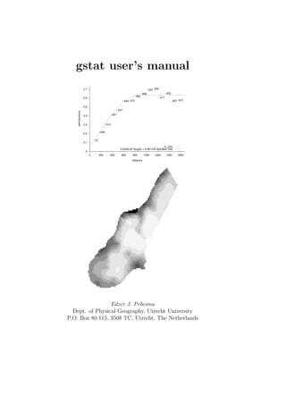
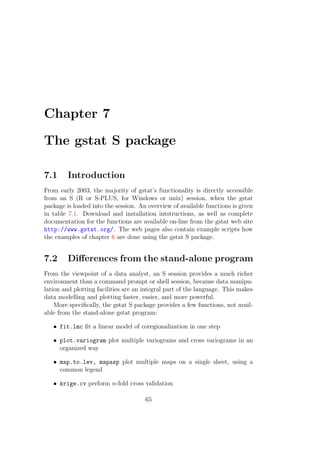
This document provides a user manual for gstat, a program for geostatistical modeling, prediction, and simulation of spatial data in one, two or three dimensions. Gstat allows for variogram modeling, kriging (prediction), and simulation using a variety of methods. It supports many data formats and provides a flexible command language for controlling geostatistical analyses. The manual describes the capabilities and proper use of the gstat program.


![14 CHAPTER 2. GETTING STARTED
Sometimes it is necessary to override the default program action (e.g. to
calculate variograms non-interactively, or to do simulation instead of predic-
tion). Information about overriding the default program action is found in
sections 2.4, 2.6 and 4.5.
2.4 Modelling spatial dependence
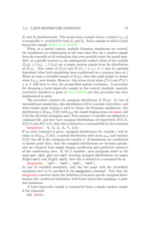
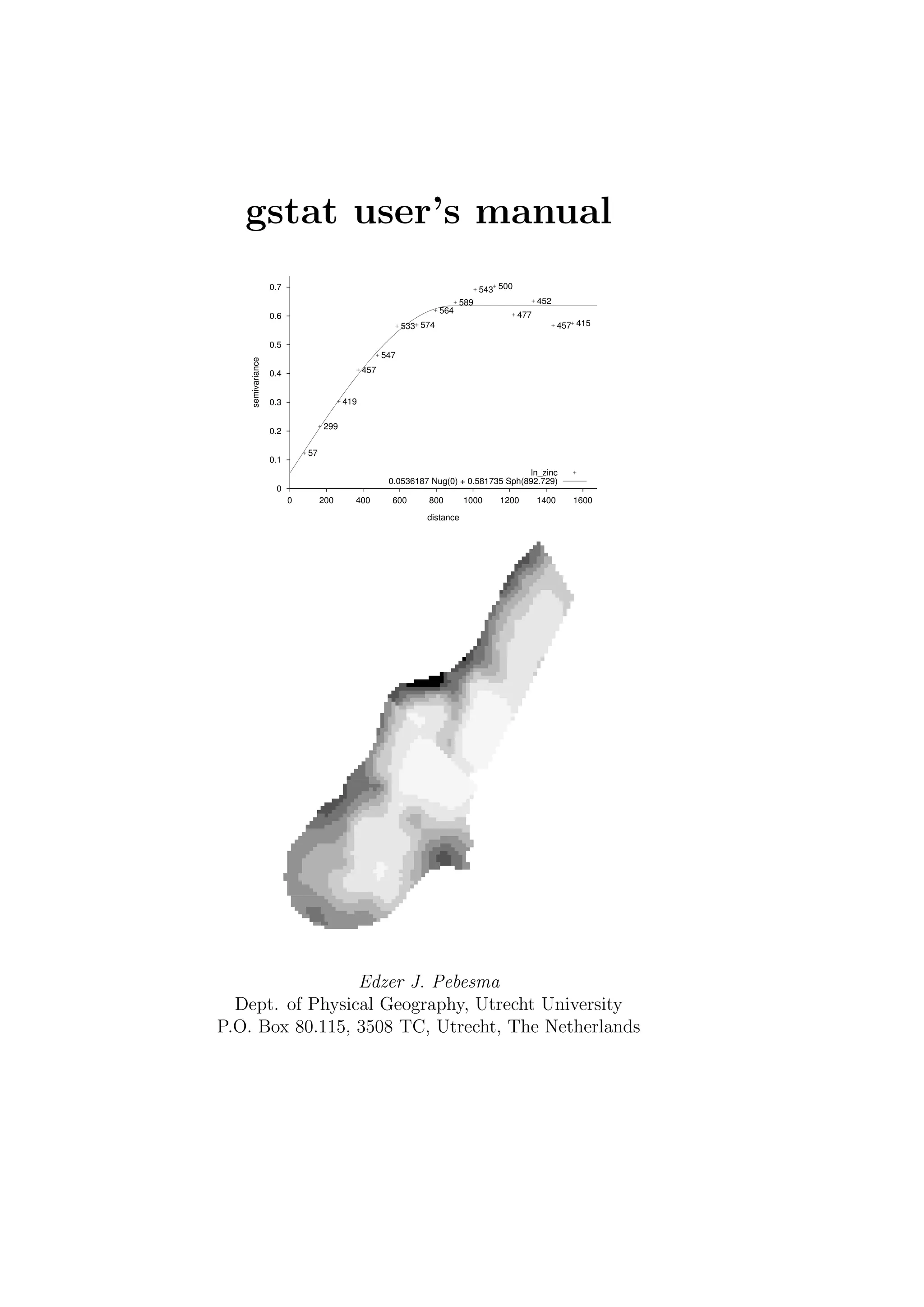
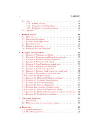
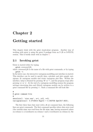
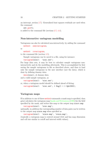
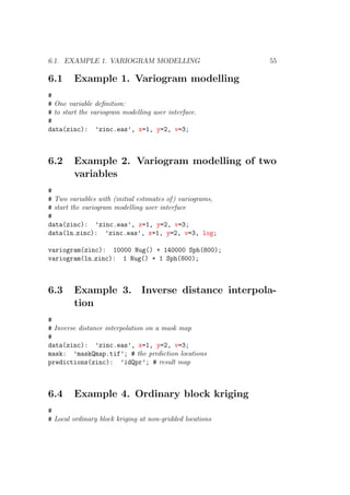
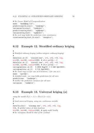
When no prediction locations are defined in the command file, gstat starts
the interactive variogram modelling user interface (example [6.1], example
[6.2]). Multiple variables are analyzed when they are specified with data(id )
commands, each having a unique id. From this interface sample variograms,
covariograms, cross variograms and cross covariograms can be calculated,
viewed, and modelled (see Appendix A.1); variogram plots can be saved (e.g.
as PostScript file, Fig. 2.2) and printed; and modified settings of data and
fitted variograms can be saved as a gstat command file. The interface has
several selection items and single-key options. Summary help is obtained by
pressing ‘H’ (shift-h).
0
0.1
0.2
0.3
0.4
0.5
0.6
0.7
0 200 400 600 800 1000 1200 1400 1600
semivariance
distance
57
299
419
457
547
533 574
564
589
543 500
477
452
457 415
ln_zinc
0.0536187 Nug(0) + 0.581735 Sph(892.729)
Figure 2.2: Variogram plot from gnuplot
Help on a specific user interface item is obtained by selecting the item
with the cursor keys and pressing ‘?’. What follows is a brief description of
the visible items in the user interface:](https://image.slidesharecdn.com/gstat-160607011055/85/Manual-Gstat-14-320.jpg)
![2.5. PREDICTION 17
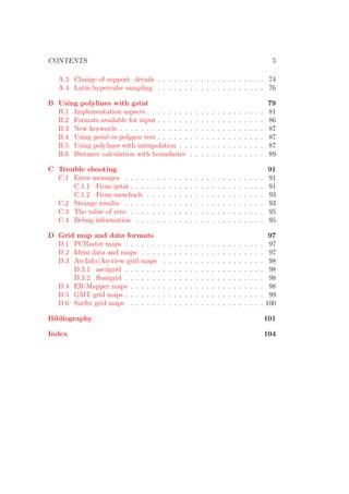
2.5 Prediction
If prediction locations are defined in the command file, gstat chooses a pre-
diction method depending on the model defined by the complete set of com-
mands in a command file.
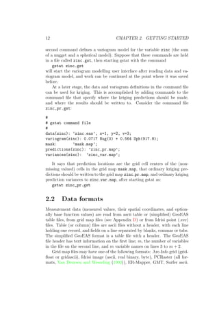
When no variograms are specified, inverse distance weighted interpolation
is the default action (Fig. 2.1, example [6.3]).
When variograms are specified the default prediction method is ordinary
kriging Journel and Huijbregts (1978); Cressie (1993) (example [6.4] and
example [6.8]).
Simple kriging is the default action when in addition for each variable the
simple kriging mean (sk mean or b) is set (section 4.2; example [6.5], universal
kriging or uncorrelated linear model prediction is used when a model for the
trend is defined ,section 2.7). Multiple prediction, multivariable prediction,
and stratified prediction are described in section 3.1-3.4. Prediction of block
averages is described in section 3.5.
If the prediction locations are specified as a mask map with the command
mask: ’file’;
then predictions and prediction variances are written to output maps only
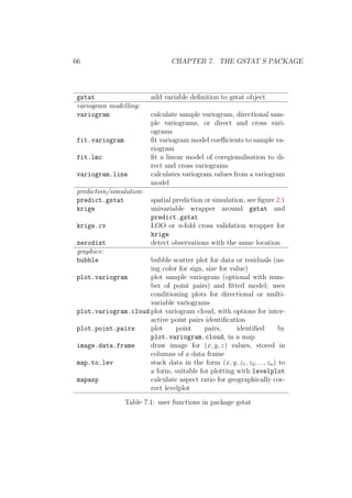
when these maps are specified explicitly (section 4.1; example [6.5]).
As an alternative to prediction on grid map locations, prediction on non-
gridded locations is the default action when these locations are specified with
the
data(): ... ;
command (note the absence of an identifier between the parentheses). In
this case, output is written in ascii table or simplified GeoEAS format to the
file defined by the command set output=’file’; (example [6.4], or defined
with the command line option -o, section 5.2).
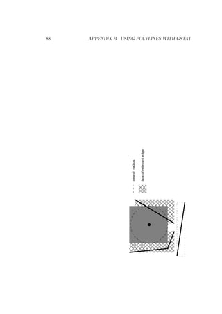
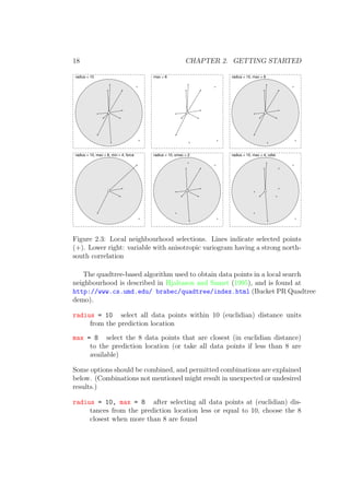
Local Neighbourhoods
By default, gstat uses global prediction, meaning that for each prediction
all data values are used. However, it is often desirable to use not all data
values, but only a subset in a (spatial) neighbourhood around the prediction
(simulation) location, for either computational reasons or the wish to assume
first-order stationarity only locally. Gstat allows local neighbourhood selec-
tions to be based on distance (radius), number of data points (max, min),
variogram distance (vdist), and number of data points per octant (3D) or
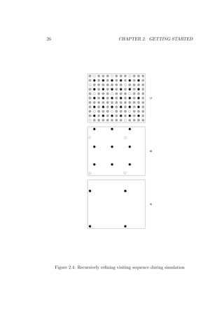
quadrant (2D) (omax). The options are explained below (see also Fig. 2.3,
section 4.2 examples in chapter 6).](https://image.slidesharecdn.com/gstat-160607011055/85/Manual-Gstat-17-320.jpg)
![2.6. SIMULATION 19
radius = 10, max = 8, min = 4 in addition to the previous selection,
generate a missing value if less than 4 points are found within the
search radius 10
radius = 10, max = 8, min = 4, force in addition to the previous se-
lection, if less than 4 data points are found in the search radius, instead
of generating a missing value, select (force) the 4 nearest (in euclidian
distance) data points, regardless their distance
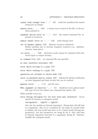
radius = 10, omax = 2 after selecting all data points at distances less
or equal to 10, choose the 2 closest data points in each octant (3D),
quadrant (2D) or secant (1D)
radius = 10, vdist, ... after the radius selection, decide what the near-
est data points are on the base of point-to-point semivariance of the
data variable instead of euclidian distances (“semivariance distance”:
in case of anisotropy this allows the prevalence of more correlated points
over the, in the euclidian sense, nearest points)
Indicator kriging
Basically, indicator kriging is equivalent to simple or ordinary kriging of
indicator-transformed data. However, resulting estimates of indicator values
are not guaranteed to satisfy order relations. During indicator kriging, gstat
will do order relation violation correction for independent, cumulative or
categorical (disjunct) indicators only if the order is to one of the values in
Table 2.1 in section 2.6, order in section 4.4 and Deutsch and Journel (1992);
Goovaerts (1997).
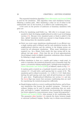
2.6 Simulation
Simulation Davis (1987); G´omez-Hern´andez and Journel (1993); Myers (1989)
is done by setting up a command file for simple kriging (section 2.5) and
changing the default action to Gaussian simulation by adding the command
method: gs;
(example [6.6] and example [6.7]), or to indicator simulation by adding the
command
method: is;
If valid data are present (i.e., data are available in the neighbourhoods de-
fined), conditional simulation is done. Unconditional simulation is done when
only dummy variables (dummy, section 4.2) or data outside every possible
neighbourhood are defined.](https://image.slidesharecdn.com/gstat-160607011055/85/Manual-Gstat-19-320.jpg)
![2.7. LINEAR MODELS IN GSTAT 23
which can be written in matrix notation as
Z(s) = Fβ + e(s) (2.3)
with F = (f1(s), ..., fp(s)) and β = (β1, ..., βp) . Ordinary kriging (2.1) is the
special case where this model has only an intercept (p = 1, f1(s) = 1, ∀x and
β1 = m).
Gstat calculates prediction under the multivariable universal kriging model
Ver Hoef and Cressie (1993) when base functions fi(s) and variogram(s) for
e(s) are specified (see appendix A.2 for the prediction equations). An inter-
cept (the constant value as in the ordinary kriging model) in (2.1) is assumed
for each variable by default, and only non-intercept base functions need to
be specified. Base functions can be polynomials of the coordinates (e.g. x,
x2
, xy etc.) or user-defined.
Coordinate polynomial base functions
For a data variable in two dimensions, a first order linear trend in the coor-
dinates is defined by
data(x): ’file’, x=1, y=2, v=3, X=x&y;
or, as a shorthand for this, the coordinate polynomial trend order degree can
be specified:
data(x): ’file’, x=1, y=2, v=3, d=1;
(Note that d=1 is equivalent to X=x for one-dimensional, X=x&y to for two-
dimensional and to X=x&y&z for three-dimensional data.) Values of coordi-
nate polynomial base functions at observation and prediction locations are
obtained from the (standardised) location coordinates si (see also example
[6.18]).
User-defined base functions
Non-coordinate polynomial, user-defined functions can also be specified as
base functions. Because they are not known, they should be defined as
column numbers in a data file (example [6.13]), like
data(x): ’file’, x=1, y=2, v=3, X=4&5;
User-defined and coordinate polynomial base functions may be intermixed.
When binary (e.g., 0/1) variables are used as base functions, and the
sum of these functions coincides with an intercept (i.e., summed row-wise,
the columns equal a column with a constant), the default intercept has to be
overridden. This is done by specifying -1 as the first column number of the
base functions (example [6.14]).](https://image.slidesharecdn.com/gstat-160607011055/85/Manual-Gstat-23-320.jpg)
![24 CHAPTER 2. GETTING STARTED
Specification of the user-defined base function values at prediction loca-
tions is necessary, since they are needed in the prediction. For the prediction
locations they are needed too, and for map prediction locations they are de-
fined as a list of mask maps containing the base functions. For the data()
prediction locations they are defined as the X column numbers in the corre-
sponding file. In both cases the number of base functions thus specified and
the order in which they appear should match the order in which the (non-
intercept and non-coordinate polynomial) X columns appear in subsequent
data(id ) commands.
If more than one variable is defined and only direct variograms are spec-
ified, multiple universal kriging is done. If in addition to direct variograms
cross variograms are specified, multivariable universal kriging is done Ver Hoef
and Cressie (1993) (universal cokriging, section 3.3).
Ordinary and weighted least squares trend prediction
If base functions are specified but no variograms are specified, the default
prediction method is the (multiple) regression prediction, (ordinary least
squares, OLS) assuming that the e(s) are independently identically dis-
tributed (IID). In this case the prediction variance is the classical regres-
sion prediction variance for a single observation (example [6.16] and example
[6.18]), or for the mean value when the block size is non-zero (section 3.5).
If the errors are assumed to be independent with different variances, viσ2
then specifying the constants vi will result in weighted least squares (WLS)
prediction. The values vi are not variances but merely relate an individual
residuals variance to σ2
. For instance, if an observation is an average of ni
measurements, then, assuming the variance of individual measurements is
constant, vi can be set to n−1
i . In the unweighted case, all vi are 1, and for
prediction variances to make sense, the vi should be related to this unity
value (σ2
should be “the” residual variance).
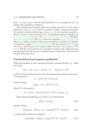
Generalised least squares trend prediction
If at prediction locations s0, for some reason not the kriging prediction but the
generalised least squares estimate (or BLUE, best linear unbiased estimate) of
the trend f(s0)ˆβ and its estimation variance are needed, then this is obtained
by overriding the default method (ordinary or universal kriging) using
method: trend;
Setting fi(s0) to 1 and all other f(s0) to 0 yields the generalised least squares
estimate (BLUE) of ˆβi. See appendix A.2 for details on weighted or combined
weighted and generalised least squares prediction.](https://image.slidesharecdn.com/gstat-160607011055/85/Manual-Gstat-24-320.jpg)

![Chapter 3
Prediction modes and change
of support
3.1 Modes
When a command file holds more than one variable, each specified with
a unique id, then different prediction (or simulation) modes are possible,
depending on the complete model specification: predictions can be made in-
dependently (‘multiple’ prediction), dependently (‘multivariable’ prediction),
or variables may correspond to certain portions (categories) in the mask map
or prediction location data (‘stratified’ prediction). The modes hold equally
for prediction and simulation. When only one variable is defined, predic-
tions (or simulations) are made for this variable at every prediction location
(‘simple’ mode).
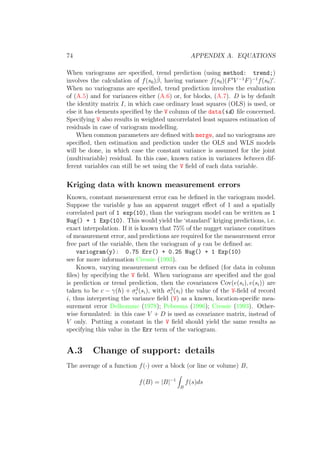
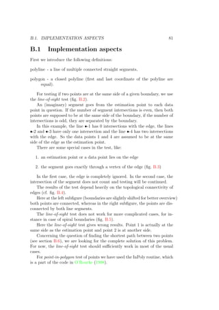
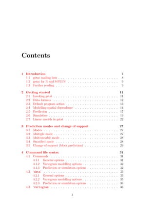
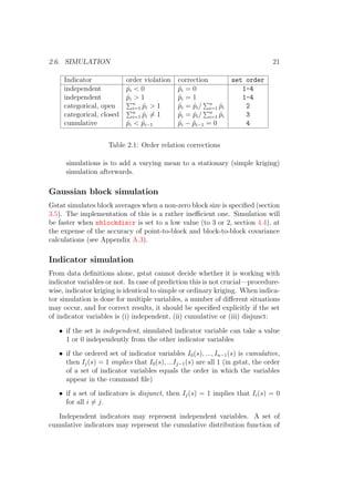
The decision tree gstat uses to determine the mode is shown in Fig. 3.1.
The choice for a certain mode is always implicit, and is made after gstat read
the command file and examined the data.
3.2 Multiple mode
When multiple variables are defined, and no variograms or only direct vari-
ograms are defined (no cross variograms), then multiple prediction (simula-
tion) is the default action. See for instance example [6.10]. In the multiple
mode, predictions or simulations are made for each variable independently.
The advantage of using the multiple mode over using a command files for
each variable, is that, besides being concise, if the variables have identical
locations, each neighbourhood search is done only for the first variable (ex-
ample [6.17]).
27](https://image.slidesharecdn.com/gstat-160607011055/85/Manual-Gstat-27-320.jpg)
![28 CHAPTER 3. PREDICTION MODES AND CHANGE OF SUPPORT
Multiple variables present?
No
Simple
Yes
All crossvariograms defined? Multivariable
Yes
No
Number of strata > 1? Multiple
No
Yes
Stratified
Mode:Condition:
Figure 3.1: Prediction modes
3.3 Multivariable mode
If in addition to direct variograms the cross variograms are defined for all
variable pairs, then the prediction mode becomes multivariable (i.e., cokrig-
ing or co-simulations). In case of multivariable prediction, prediction error
covariances from multivariable prediction Ver Hoef and Cressie (1993) on a
map can be specified per identifier pair with covariances(id1,id2 ) (ex-
ample [6.11]). In gstat, multivariable prediction comprises simple cokriging,
ordinary cokriging or universal cokriging (as well as standardised cokriging,
multivariable indicator or Gaussian simulation).
When, for multiple variables a linear model is specified with indepen-
dent errors (no variograms are defined), and one or more of the variables’
regression parameters are defined as common parameters (with the command
merge, section 4.1) then the prediction mode becomes multivariable as well
(cf. analysis-of-covariance models refXXchristensen96).
3.4 Stratified mode
Stratified kriging or simulation (each variable with it’s direct variogram ap-
plies to a specific area in the mask map) is the default action if the following
conditions hold (example [6.12]):
• more than one data variable is defined
• only for the first data variable output maps (predictions, variances)
are defined](https://image.slidesharecdn.com/gstat-160607011055/85/Manual-Gstat-28-320.jpg)
![3.5. CHANGE OF SUPPORT (BLOCK PREDICTION) 29
• the (first) mask map defined has more than one category
Data variables are numbered in the order they appear in the command
file, starting at 0. Let the minimum grid value of the (first) mask map be
m, If at a specific grid cell the mask map has value j, then for that cell
the stratified prediction map (and variance map) will have predictions for
variable j − m (rounded to the nearest integer). Thus, predictions at mask
map cells having value m will get predictions for the first variable.
In case of universal kriging or least squares prediction with user-defined
base functions, the maps with base function values should follow the category
map: in the stratified mode the first mask map is the map with the categories.
3.5 Change of support (block prediction)
Average values for square, rectangular or arbitrarily shaped blocks can be
predicted in gstat for all kriging variants, for OLS or WLS prediction or
for inverse distance weighted interpolation, or they can be simulated using
multi-Gaussian simulation.
The mean value of a block, the size of a grid cell, is obtained by adding
the command
blocksize;
to the command file. Alternatively, block mean values for rectangular blocks
with arbitrary size, centred at prediction locations are obtained when the
block size is specified, in one dimension:
blocksize: dx = 1;
for a line element with length 1, in two dimensions
blocksize: dx = 1, dy = 2;
for a rectangular element with size 1 × 2 or in three dimensions
blocksize: dx = 1, dy = 2, dz = 3;
for a block with dimensions 1 × 2 × 3, see example [6.4] and example [6.8].
Block averages are approximated by discretizing (“representing”) the
block with a limited number of points Journel and Huijbregts (1978); Carr
and Palmer (1993). Blocks with arbitrary shapes may be defined by specify-
ing the points discretizing the block (see appendix A.3).](https://image.slidesharecdn.com/gstat-160607011055/85/Manual-Gstat-29-320.jpg)

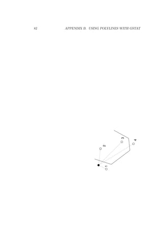
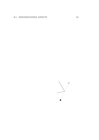
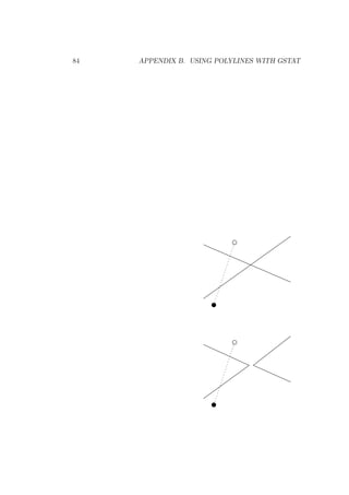
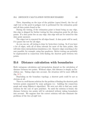
![4.2. ‘DATA’ 33
point is on the same side of an edge as the prediction location, it will
be included for prediction (or simulation). See Appendix B for details
and polygon file formats.
area: body; here, body defines the ‘block’ discretization points (section
3.5, Appendix A.3)
merge id1(i ) with id2(j ); In multivariable ordinary or universal krig-
ing (or simulation), by default each variable has it’s own set of pa-
rameters βk. The merge command allows to define a common pa-
rameter for two or more variables. Suppose, Z1(x) = m + e1(x) and
Z2(x) = m + e2(x), where m is the unknown common mean for both
variables. Note: the variable numbers i and j start at 0; merge id1
with id2 is the abbreviation of merge id1(0) with id2(0) (see also
Appendix A.2).
4.2 ‘data’
The general form of the data command is
data(identifier): ’file’, options ;
The file name should refer to an existing file in ascii table form, simplified
GeoEAS format or one of the supported grid map formats. Options can
be single keywords like log or expressions like x=2. Column 0 means not
defined (non-existent). The full list of options is [default values between
square brackets]:
4.2.1 General options
v=5 column 5 contains the data (measurement) variable [0, or obtained
from grid map]
x=1 column 1 contains the x-coordinate [0, or obtained from grid map]
y=2 column 2 contains the y-coordinate [0, or obtained from grid map]
z=3 column 3 contains the z-coordinate [0, or obtained from grid map]
d=1 use a first order (polynomial) linear model in the coordinates as the
trend; allowed order values are 0, 1, 2 and 3; see also X, sk mean and b
[0: only an intercept as trend]
mv=-1 define missing value as the value -1 [the string NA, see also set mv]](https://image.slidesharecdn.com/gstat-160607011055/85/Manual-Gstat-33-320.jpg)
![34 CHAPTER 4. COMMAND FILE SYNTAX
average average values with identical locations (i.e., their separation dis-
tance is less than zero) [noaverage]
log log transform the variable (natural logarithm) [no transform]
I=5 transform the observation variable v to
I(v, 5) =
1 if v ≤ 5,
0 otherwise
[no transform]
v=6, Category=’sand’ transform the observation variable v to 1 if the
string in column 6 equals the Category string sand, and to 0 in any
other case. [no transform]
ns=’filename.out’ transform the observations to their normal score, and
write the normal score table to filename.out. In this file, ach line
contains the (sorted) original value and its normal score. Normal scores
are computed as
nj(xi) = Φ−1
((j + 0.5)/n)
with j the rank (1...n) of z(xi) and Φ(·) the Gaussian cumulative density
function. In case of ties (when multiple z(xi) have the same value),
ranks are averaged for the tied data before normal scores are calculated,
to avoid assignment of arbitrary values. Gstat does (currently) not
provide any means for backtransformation.
standard standardise variable (to mean 0, variance 1) [do not standardise]
X=8&9&x&y apart from a default intercept, the values of the base functions
at the data locations are the variables that are in columns 8, 9 and the
x- and y-coordinate. (Polynomial coordinate base functions allowed
are: x3 for x3
, y3 for y3
, z3 for z3
, x2 for x2
, y2 for y2
, z2 for z2
, x for
x, y for y, z for z, x2y for x2
y, xy2 for xy2
, x2z for x2
z, xz2 for xz2
, y2z
for y2
z, yz2 for yz2
, xy for xy, xz for xz and yz for yz, provided that
the corresponding coordinate is defined) [use only an intercept (mean)
as trend]
X=-1&8&9 the values of the base functions at the data locations are on
columns 8, 9 and 10, with no intercept [use only an intercept (mean)
as trend]](https://image.slidesharecdn.com/gstat-160607011055/85/Manual-Gstat-34-320.jpg)
![4.2. ‘DATA’ 35
b=[2.4, 1.7, -3.9] define the (known) regression coefficients, correspond-
ing to the X entries given. See also sk mean; b generalises the concept
of a known constant mean to a known mean function. [undefined; re-
gression coefficients are unkonwn]
V=6 column 6 contains the proportionality factor vi to the residual vari-
ance viσ2
of the v-variable (i.e. the diagonal entries of matrix D, see
Ordinary and weighted least squares trend prediction in section 2.7, and
Appendix A.2). This will have an effect on the least squares residuals
(thus affecting the sample covariogram and pseudo cross variogram), as
well as on uncorrelated least squares prediction, kriging prediction, and
trend prediction. [0: assuming identical variances or variances strictly
derived from the variograms]
every=10 For regular (systematic) sampling records from a data file, every
is set to the step size. A value of 10 only samples data records 1, 11, 21, ...
[1: don’t sample but select all data]
offset=1 Controls the starting sample element for regular sampling. Effec-
tive in combination with every only. When every=10 and offset=2,
then elements 2, 12, 22, ... are selected; if every=20 and offset=5, ele-
ments 5, 25, 45, ... are selected. [1: start sampling at first data point].
prob=0.1 Inclusion probability for random sampling data records from the
file [1: all records are read].
4.2.2 Variogram modelling options
noresidual do not calculate OLS (or GLS, see gls) residuals for sample
variogram or covariogram estimation (Appendix A.1). For sample vari-
ogram estimation in absence of base functions, setting noresidual will
yield identical results, but will result in a modest gain in speed and
memory saving. In other cases, it will result in the estimation of non-
centred covariograms or pseudo-cross variograms [calculate residuals
before variogram or covariogram estimation]
dX=0.1 include a pair of data points {z(xi), z(xj)} for sample variogram
calculation only when ||f(xi)−f(xj)|| ≤ 0.1 with f(xi) = (f1(xi), ..., fp(xi))
and ||u|| =
√
u u. This allows pooled estimation of within-strata vari-
ograms, or variograms of (near-)replicates in a linear model (for point
pairs having similar values for regressors like depth, time, or a category
variable) [do not evaluate]](https://image.slidesharecdn.com/gstat-160607011055/85/Manual-Gstat-35-320.jpg)
![36 CHAPTER 4. COMMAND FILE SYNTAX
4.2.3 Prediction or simulation options
radius=4.5 select observations in a local neighbourhood when they are
within a distance of 4.5 [large: select all] (see section 2.5)
max=30 maximum number of observations in a local neighbourhood selec-
tion is 30 [large: no maximum] (see section 2.5)
min=10 minimum number of observations in a local neighbourhood selec-
tion is 10 [0] (see section 2.5)
omax=2 maximum number of observations per octant (3D), quadrant (2D)
or secant (1D) is 2 (this only works in addition to a radius set) [0:
don’t evaluate] (see section 2.5, and also method: nr;, section 4.5)
square select points in a square (or block) neighbourhood, with square
(block) sizes equal to 2 × radius [circular (spherical) neighbourhood]
vdist use variogram value as the distance criterium for min/max/omax
neighbourhood selection (but define radius as euclidian distance) [use
Euclidean distance] (see section 2.5)
force force neighbourhood selection to the minimum number of observa-
tions, disregarding the distance [unless simple kriging is used, generate
a missing value if less than the required minimum number of obser-
vations are found within a distance defined by radius] (see section
2.5)
s=7 define variable with the strata for data() locations [0, no strata]
sk mean=2.4 define the simple kriging mean to be 2.4 [not defined: an
unknown mean (intercept) is assumed for each variable]. NOTE: the
code sk mean=2.4 is equivalent to b=[2.4]
dummy define a dummy variable [require valid data to be read]
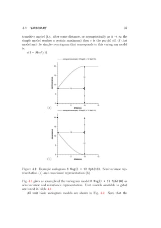
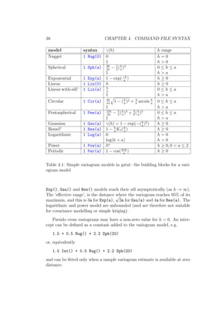
4.3 ‘variogram’
Variogram models are coded as the sum of one or more simple models (and
optionally an anisotropy structure). A simple variogram model is denoted
by
c Mod(a)
with c the vertical (variance) scaling factor, Mod the model type, and a the
range (horizontal, distance scaling factor) of this simple model. If Mod is a](https://image.slidesharecdn.com/gstat-160607011055/85/Manual-Gstat-36-320.jpg)
![4.4. ‘SET’ 41
The list of variables that can be ‘set’ [default value between brackets]:
4.4.1 General options
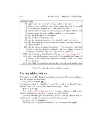
set debug=2; set debug level to 2 [1; options are listed in Appendix C.4]
set cn max=1.0e8; check the condition number of matrices. If it is larger
than cn max, then generate a missing value and report a (near) sin-
gularity warning. Matrices checked are V and F V −1
F (or F D−1
F).
A suitable value for cn max seems 1/
√
DBL EPSILON, which is about
108
. Condition numbers are estimated using LU factorization Stewart
and Leyk (1994), and may be an order of magnitude wrong. Condition
numbers are reported if debug is set to report covariance matrices. [not
set: check for singularity only during variogram model fitting]
set logfile=’gstat.log’; set the file name where debug information is
written to (see set debug and Appendix C.4) [stdout, debug informa-
tion is written to the screen]
set mv=’MisVal’; define the default missing value string as MisVal [the
string NA] (Note that numerical missing values can be defined with mv
in a data command)
set output=’file’; write ascii output to file (e.g., variogram estimates,
predictions and variance at non-gridded locations)
set plotfile=’file’; file defines the file name for gnuplot commands
(not set, use temporary files). When set during ordinary or univer-
sal kriging, kriging weights are written as plot files for gnuplot (see
plotweights). Affects file name usage for variogram plotting through
gnuplot.
set zero=1.0e-10; specify the highest value absolote differences in dis-
tance and prediction variances may have to be considered equal to zero
[10 × DBL_EPSILON, about 2−15
].
set marginals=list; List of values or maps with the mean and variance
of the first variable, the second variable, ... See also section A.4.
4.4.2 Variogram modelling options
set alpha=45.0; directional sample (co-) variogram: set direction in <
x, y > plane, in positive degrees clockwise from positive y (North) [0.0]](https://image.slidesharecdn.com/gstat-160607011055/85/Manual-Gstat-41-320.jpg)
![42 CHAPTER 4. COMMAND FILE SYNTAX
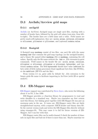
set beta=30.0; directional sample (co-) variogram: set direction in z, in
positive degrees up from the < x, y > plane [0.0]
set Cressie=1; (for sample variogram calculation) use Cressie’s square-
root variogram estimator [0]
set cutoff=0.5; set cutoff (max. dist. for sample variogram) at 0.5 [a
fixed fraction of the maximum distance, see set fraction]
set dots=1000; change the number of plotting points at which gstat will
let gnuplot switch from plotting points (+) with numbers of points of
pairs, to plotting dots without numbers [500]
set fit=1; fit the variogram model to the experimental variogram, using
weighted least squares fit. Values for fit are shown in table 4.2 [0, do
not fit]
fit fit by weight
0 - - (no fit)
1 gstat Nj
2 gstat Nj/{γ(hj)}2
3 gnuplot Nj
4 gnuplot Nj/{γ(hj)}2
5 gstat REML
6 gstat no weights (OLS)
7 gstat Nj/h2
j
Table 4.2: values for fit
set fit limit=1.0e-10; set fit limit to 1.0e-10 (Appendix A.1) [1.0e-6]
set format=’%.3g’; the format used for real values in variograms, e.g.
%.3g limits the number of significant digits shown to 3. A valid C-
language format string for a double should be used, misspecification
may result in unpredictable behaviour. [%g : use 6 significant digits]
set fraction=0.25; specify the default cutoff for sample variogram cal-
culation as fraction of the length of the diagonal in the square or block
spanning the data locations [0.333]
set gnuplot=’mygnuplot’; invoke the program mygnuplot as gnuplot
(variogram display) [gnuplot, or wgnuplot for Win32]](https://image.slidesharecdn.com/gstat-160607011055/85/Manual-Gstat-42-320.jpg)
![4.4. ‘SET’ 43
set gnuplot35=’gpt35’; invoke the program gpt35 (gnuplot version 3.5)
for variogram display only [use gnuplot, or the value of set gnuplot]
set gpterm=’latex’; set the gnuplot terminal specification and options
(a string to follow the gnuplot “set term” command). This option will
overrule the ‘postscript’ or ‘gif’ settings from the variogram modelling
user interface, thus allowing plotting to other graphic file formats and
modification of options (see gnuplot documentation). [for gif: ’gif
transparent size 480, 360’, for PostScript: ’postscript eps
solid 17’
set intervals=20; specify the default number of intervals for sample va-
riogram calculation [15]
set iter=20; use not more than 20 iterations on iterative fit methods [50]
set pager=’less’; use ‘less’ as pager to be called from the variogram
modeling interface [the value of the environment variable PAGER (if
set), or else the program more]
set secure=1; prevent any calls to the functions system(), popen() or
remove(), terminate program whenever one of the first two appear
(once set, it cannot be set back) [0, not secure]
set sym=1; force directional sample cross covariance and pseudo cross
semivariance to be symmetric [0, asymmetric]
set tol hor=45.0; directional sample (co-)variogram: set horizontal tol-
erance angle in degrees [90.0]
set tol ver=20.0; directional sample (co-) variogram: set vertical toler-
ance angle in degrees [90.0]
set width=0.05; set lag width to 0.05 (distance interval width for sample
variogram) [cutoff/intervals]
set gls=1; use generalised least squares residuals instead of the default
ordinary least squares (OLS) residuals for sample variograms or covar-
iograms [0, use OLS or WLS residuals]
set zero dist=1; determine what happens with variogram estimates at
distance zero. Values are 1: include in first interval, 2: omit, 3: calcu-
late separately [1 for variograms, 3 for covariograms]](https://image.slidesharecdn.com/gstat-160607011055/85/Manual-Gstat-43-320.jpg)
![44 CHAPTER 4. COMMAND FILE SYNTAX
4.4.3 Prediction or simulation options
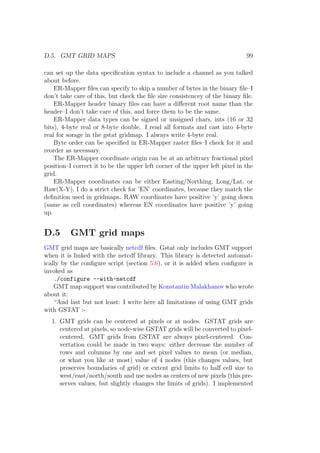
set idp=3.5; set inverse distance power to 3.5 [2]
set nblockdiscr=10; use regular block discretization with 10 points in
each dimension at non-zero block size (note: 10 in 3 dimensions results
in 1000 discretizing points) [4, and use Gauss quadrature (see Appendix
A.3)]
set nsim=100; create 100 independent simulations when following a single
random path (output maps will get the simulation number attached to
their names, therefore short names should be chosen in environments
with file name restrictions) [1]
set n uk=40; (for conditional simulation only) use universal (or ordinary)
kriging instead of simple kriging when the number of data in a kriging
setting is greater than or equal to 40. For multivariable prediction
the neighbourhood size is summed over all variables, otherwise it is
evaluated per variable. Setting n uk to zero limits use of simple kriging
to empty neighbourhoods only [very large: always use simple kriging]
set order=2; define the action when order relation violations occur during
indicator simulation (section 2.6; table 2.1) or indicator kriging (section
2.5). Values are 0: no correction for indicator kriging, assure that
estimated probabilities are in [0,1] before simulation; 1: as 0, but also
for indicator kriging; 2: rescale the estimated probabilities if their sum
is larger than 1; 3: rescale the estimated probabilities so that they
sum up to 1; 4: do order relation correction for cumulative indicators
(using the upward-downward averaging steps of GSLIB Deutsch and
Journel (1992)). [0: do only basic order relation violation corrections
for indicator simulation]
set plotweights=10; When plotfile is set, kriging weights will be plot-
ted during ordinary or universal kriging. If plotweights is larger than
1, data point sizes are proportional to kriging weights using size inter-
vals of 1
plotweights. If not (default), kriging weights are plotted as
data point labels (i.e., as text).
set quantile=0.25; when method was set to med, report p-quantile of
local neighbourhood selection as prediction value, and (1 − p)-value as
prediction variance [0.5: the median]
set rp=0; follow regular, non-random path during sequential simulation
[1, follow a random path]](https://image.slidesharecdn.com/gstat-160607011055/85/Manual-Gstat-44-320.jpg)
![4.5. ‘METHOD’ 45
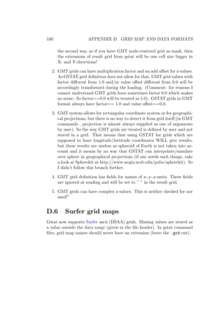
set seed=1023; set seed for random number generator [0: seed is read
from the internal clock. If possible, microseconds are used. To check
this, run gstat a few times with debug set to 2].
set useed=4053341103U; set seed for random number generator when
outside the range of a signed integer; note the ‘U’ at the end of the
number [see seed].
set sparse=10; Use sparse matrix routines for covariance matrix. The
number of sparse should be a reasonable estimate of the number of
non-zero columns in each row of the covariance matrix V . [only avail-
able when sparse matrix routines in meschach are linked in; 0: use
dense matrices]
set xvalid=1; turn cross validation on (if prediction is possible) [0, no
cross validation]
set zmap=10.0; set height of mask map(s) to 10 when observations are
3-D. [0.0]
set lhs=1; Apply Latin hypercube sampling to Gaussian simulations; see
also marginals
set nocheck=1; Ignore error in case of an non-permitted coregionalisation
(intrinsic correlation or linear model of coregionalisation)
4.5 ‘method’
Values for method that make gstat deviate from the default action are:
gs override the default kriging method to get Gaussian simulations (section
2.6)
is override the default kriging method to get indicator simulations (section
2.6)
semivariogram sample semivariance on output (see also fit, section 4.4)
covariogram sample covariogram on output
trend spatial trend estimation (x0
ˆβ), using generalised least squares if var-
iograms are specified, or else using ordinary or weighted least squares
(see Appendix A.2)](https://image.slidesharecdn.com/gstat-160607011055/85/Manual-Gstat-45-320.jpg)
![46 CHAPTER 4. COMMAND FILE SYNTAX
map report the value of m mask maps at the prediction location of data()
as the output values, provided that n (dummy) input variable are de-
fined, with n ≥ m/2 (example [6.9])
distance report distance to nearest observation as the predicted value,
and the distance to the most distant observation (in the neighbourhood
selection, if defined) as prediction variance
nr report number of observations in neighbourhood as predicted value,
and, if omax was set, the number of non-empty octants (or quadrants)
as prediction variance
div diversity (the number of distinct values) in a local neighbourhood is
reported as the predicted value, the modus of the values (the value that
occurred most often in a local neighbourhood) is reported as prediction
variance
med local median or quantile estimation, see quantile in section 4.4; for
minimum and maximum values in each local neighbourhood, set quantile
to 0.0.
skew report skewness as predicted value, and kurtosis as the prediction
variance value for values in a local neighbourhood. Uses methods-of-
moments estimators: Sk = 1
σ3n
n
i=1(yi − µ)3
K = 1
σ4n
n
i=1(yi − µ)4
point-in-polygon Provided a set of (closed) polygons is given with the
edges command, the (first) polygon in which the prediction location is
located is given in the output. Predicted value carries the file number
of the polygon, prediction variance the polygon number in the file. See
also Appendix B](https://image.slidesharecdn.com/gstat-160607011055/85/Manual-Gstat-46-320.jpg)
![5.4. SPECIAL FILE NAMES 49
ran3 ranf rand48 ranmar zuf slatec r250 random minstd uni uni32 vax
transputer rand random8 randu. See the GSL documentation for details.
The environment variable GSL RNG SEED may be used to override the seed
of gstat (set or default).
5.4 Special file names
Certain special file names are allowed in gstat. They enable filtering, append-
ing to files, using standard input or output streams and command output
substitution. (They will not have this effect for PCRaster file names.)
’> file’ If file exists, then append the output to file (if it is an output
file) instead of starting with a fresh file
’| file’ Open file as a pipe, either for reading or for writing
’-’ Use, instead of a disk file, for a reading process the stream stdin, or
for a writing process the file stdout
‘cmd‘ execute the shell command cmd and substitute its output for the file
name
Using pipes is at the user’s responsibility. Blindly executing command
files that contain file names with pipes to harmful commands may result
in damage (loss of files for instance). This also applies to the setting of the
gnuplot command(s), see section 4.4. Potential damage from such situations
is considered as “consumers risk”, it is comparable to renaming harmful
programs to often-used commands.
For safety reasons, the variable secure can be set to 1, which prohibits
gstat from system calls, creating pipes or deleting temporary files. Unlike
other variables, once secure is set, it cannot be set back (indeed, for secu-
rity).
As an example of using a pipe as file name, the first variable in example
[6.12] containing the data selection from zinc map.eas with a zero in column
5, could have been defined directly in terms of zinc map.eas as
data(zinc.at.0):
"| awk ’{if(NR<11||$5==0){print $0}}’ zinc_map.eas",
x=1, y=2, v=3, log, min = 20, max = 40, radius = 1000;
provided that the awk program is available.](https://image.slidesharecdn.com/gstat-160607011055/85/Manual-Gstat-49-320.jpg)
![50 CHAPTER 5. FURTHER CONTROL
5.5 Execute (-e) actions
Several simple “special actions” are available in (“linked into”) gstat. They
are invoked as
gstat -e action arguments
and are strictly controlled by command line options and arguments. A list
of available actions is obtained by calling
gstat -e
and usage for each action is printed after running
gstat -e action
without arguments. Following is a list of available actions:
cover out map in map1 in map2 ... cover several input maps into the out-
put map: substitute in out map the missing values of in map1 with the
first non-missing value found in subsequent input maps, on a cell-by-cell
basis
convert Converts grid map file from one format to another (minimal con-
verter)
nominal out map in map0 in map1 ... in mapn from multiple input grid
map files write in each grid cell of out map the number of the first map
with a non-zero value in that grid cell (a value in [0, ..., n])
map2fig convert point data or grid map data to fig (XFig/fig2dev) file.
XFig is a vector graphics editor for X-Windows that supports exporting
to numerous formats.
map2gif convert grid map file to gif file. The gif library used to generate
gif’s from maps is not distributed as part of the gstat distribution; see
http://www.boutell.com/gd/
map2png See map2gif. Modern versions of the gd library only support
PNG instead of GIF, because of the unisys license thing. If such a
version of gd is found, gstat only supports map2png to create PNG’s.
semivariogram calculate sample variogram, using command line interface
covariogram calculate sample covariogram, using command line interface
semivariance print semivariance table for a variogram model
covariance print covariance table for a variogram model](https://image.slidesharecdn.com/gstat-160607011055/85/Manual-Gstat-50-320.jpg)

![Chapter 6
Example command files
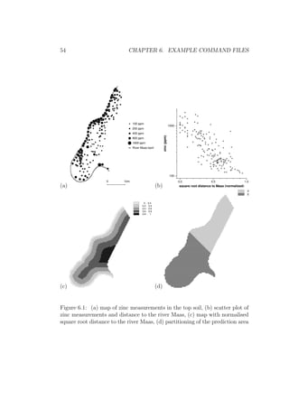
Following are the example command files, as distributed with gstat. The
data (zinc concentrations of the top soil, Fig. 6.1a) are collected in a flood
plain of the river Maas, not far from where the Maas entered the Netherlands
(Borgharen, Itteren, about 3 to 5 km North of Maastricht). All coordinates
are in metres, using the standard coordinates of Dutch topographical maps.
Moving from the river, zinc concentrations tend to decrease(Fig. 6.1b).
For the universal kriging examples, let the function D(x) be the function
that is for every location x the (normalised) square root distance to the river.
This function is physically stored for the observation locations in column 4 of
zinc map.eas (as obtained in example [6.9]), and for the prediction locations
in the map sqrtdist.map (Fig. 6.1c). The prediction area is split in two
separate sub-regions, A and B (Fig. 6.1d). Let the function IA(x) be 1 if
x ∈ A or else 0; and let the function IB(x) be 1 if x ∈ B or else 0.
The functions IA(x) and IB(x) are physically stored for the observation
locations in columns 5 and 6 of zinc map.eas, and for the prediction loca-
tions in the maps part a.map and part b.map. (Note that the partitioning
in A and B is arbitrary, it serves only illustrational purposes.)
The following command files, data and maps are distributed with gstat.
These command files are purely for illustration and as such only suggest
possible forms of analysis. Remind that everything from a # to the end of
the line is comment.
53](https://image.slidesharecdn.com/gstat-160607011055/85/Manual-Gstat-53-320.jpg)


![Appendix A
Equations
A.1 Spatial dependence
Sample variogram and covariogram
All variograms and covariograms are calculated from predicted residuals
ˆe(si) = z(si) − ˆm(si), with ˆm(si) the ordinary least square estimates of
m(si), fitted globally (all data of the variable are used in a linear model as-
suming IID errors), unless one of dX, noresidual or gls is set. The sample
variogram is calculated from residuals from a single realization z for regular
distance intervals [hj, hj + δ]. by:
ˆγ(¯hj) =
1
2Nj
Nj
i=1
(ˆe(si) − ˆe(si + h))2
, ∀(si, si + h) : h ∈ [hj, hj + δ]
with ¯hj the average of all Nj h’s. A covariogram is modeled by fitting a
model to the sample covariogram ˆC(h) calculated by:
ˆC(¯hj) =
1
Nj
Nj
i=1
ˆe(si)ˆe(si + h), ∀(si, si + h) : h ∈ [hj, hj + δ]
The sample cross variogram ˆγkl(h) is calculated from sample data by:
ˆγkl(¯hj) =
1
2Nj
Nj
i=1
(ˆek(si) − ˆek(si + h))(ˆel(si) − ˆel(si + h)),
∀(si, si + h) : h ∈ [hj, hj + δ]
The sample pseudo cross variogram gkl(h) is calculated from sample data by
ˆgkl(¯hj) =
1
2Nj
Nj
i=1
(ˆek(si) − ˆel(si + h))2
, ∀(si, si + h) : h ∈ [hj, hj + δ].
69](https://image.slidesharecdn.com/gstat-160607011055/85/Manual-Gstat-69-320.jpg)
![70 APPENDIX A. EQUATIONS
The sample cross covariogram ˆCkl(h) is calculated by the sample cross
covariance
ˆCkl(¯hj) =
1
Nj
Nj
i=1
ˆek(si)ˆel(si + h), ∀(si, si + h) : h ∈ [hj, hj + δ]
Gstat provides calculation of sample variogram, covariogram, cross vario-
gram, pseudo cross variogram and cross covariogram, where width δ, number
of intervals j and direction of h can be controlled. When some cross vario-
gram is requested, gstat decides which one should be calculated: the first,
‘classic’ cross variogram is calculated when the two variables have the same
number of observations and identical coordinates and order, in any other case
the pseudo cross variogram is calculated, this information is written to the
second line of the file with the sample variogram.
Estimation of variogram model parameters
Gstat provides several methods for estimating variogram model parameters.
Fitting of a variogram model to the sample variogram is done by iteratively
reweighted least squares (WLS, Cressie (1993)), minimizing
n
j=1
wj(ˆγ(¯hj) − γ(¯hj))2
with wj either equal to Nj or to γ(¯hj)−2
Nj.
Fixing parameters in a weighted least squares fit can be done by putting
an @ before the range or the sill parameter to fix: e.g. fitting the variogram
1 Sph(@ 0.2) will only fit the sill parameter (1), fitting @1 Sph(0.2) will
only fit the range parameter (0.2).
Within gstat, iterative fitting stops when the number of steps exceeds 50
(or the value set by iter) or when the fit has converged. A fit is considered
as ‘converged’ when the change in the weighted sum of squares of differences
between variogram model and sample variogram becomes less then 106
× the
last value of this sum of squares (this number is controlled with fit limit).
Both gstat and gnuplot fix the fitting weights during iteration. For
this reason, when the fitted model strongly differs from the initial (start-
ing) model, another fitting round may converge to a (substantially) different
model, because the variogram model, and consequently the weights, changed.
Reiterated weighted fitting may very well result in never converging cycles.
Gstat uses Gauss-Newton fitting with (mostly) analytical derivative func-
tions; gnuplot uses Levenberg-Marquardt fitting with numerical derivatives.](https://image.slidesharecdn.com/gstat-160607011055/85/Manual-Gstat-70-320.jpg)
![72 APPENDIX A. EQUATIONS
required, then for user-defined base functions the values for f(B0) should
be given as input to gstat (in the mask map(s) or in the X-columns of
the data() file), whereas point-to-block and block-to-block covariances (i.e.,
Cov(e(si), e(B0)) and σ2
Z(B0)) are derived from the point-to-point (gener-
alised) covariances, using Gaussian quadrature Carr and Palmer (1993) or,
when either nblockdiscr or area is specified, using simple integration (reg-
ular or user-specified discretization, equally weighted).
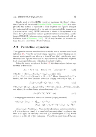
Simple kriging
When β is known, simple kriging prediction is obtained. It only involves the
prediction of e(s0):
ˆZ(s0) = f(s0)β + v0V −1
(z(s0) − f(s0)β)
having variance
Var(Z(s0) − ˆZ(s0)) = σ2
Z(s0) − v0V −1
v0
Multivariable prediction
When s variables Zk(s), k = 1, ..., m each follow a linear model Zk(s) =
Fkβk + ek(s), and the ek(s) are correlated, then it makes sense to extend the
weighted least squares model to allow multivariable prediction. Without loss
of generality, assume m = 2. When z(s) = (z1(s), z2(s)) and B = (β1, β2)
are substituted for z(s) and β, and when
f(s0) =
f1
(s0) 0
0 f2
(s0)
, F =
F1 0
0 F2
,
V =
V11 V12
V21 V22
, v0 =
v11 v12
v21 v22
with fk
(s0) the f(s0) that corresponds to variable k, with
V21 = [Cov(e2(si), e1(sj))],
v21 = (Cov(e2(s1), e1(s0)), ..., Cov(e2(sn), e1(s0))) ,
and 0 a conforming zero matrix or vector, are substituted for f(s0), F, V and
v0, then the left-hand sides of both (A.2) and (A.4) yield the multivariable
predictions: the left-hand side of (A.2) then becomes the prediction vector](https://image.slidesharecdn.com/gstat-160607011055/85/Manual-Gstat-72-320.jpg)