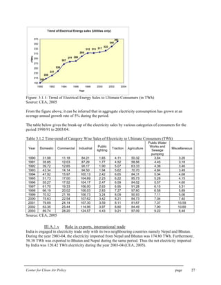
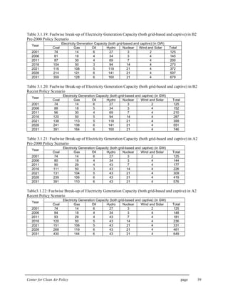
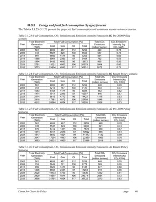
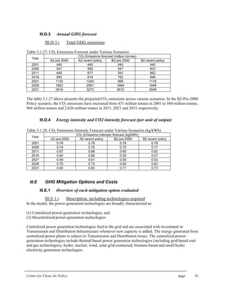
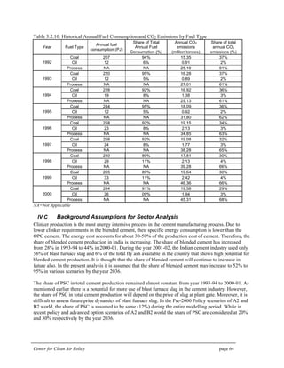
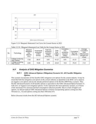
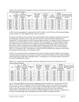
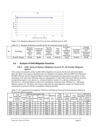
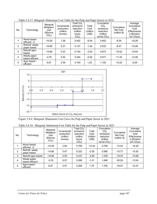
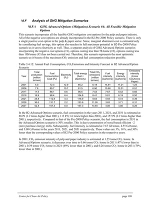
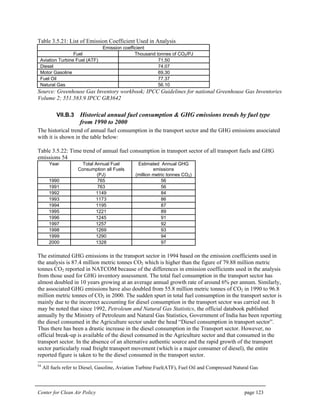
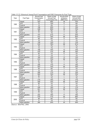
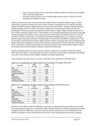
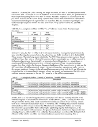
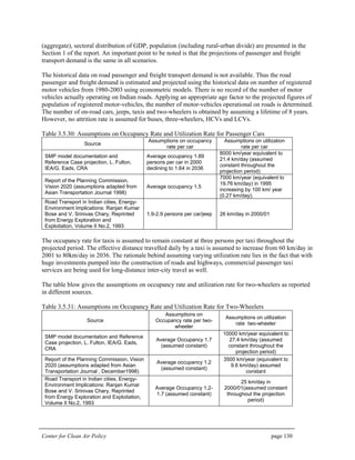
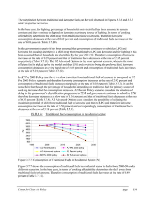
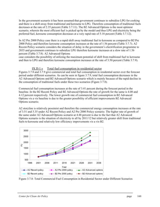
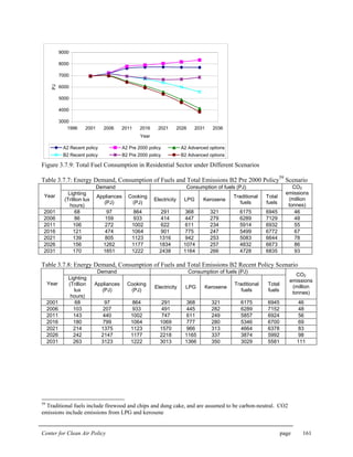
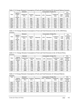
Download to read offline


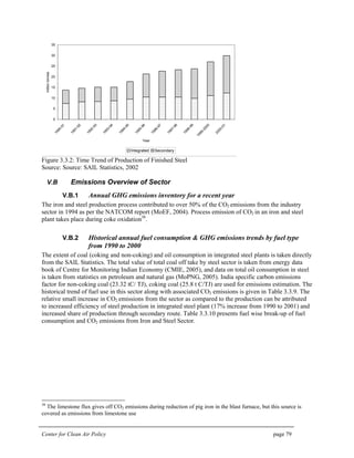
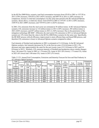


This document summarizes a report on greenhouse gas mitigation opportunities in India's electricity sector through 2031. It provides an overview of India's electricity sector, including historical energy consumption and emissions trends. Baseline forecasts predict rising electricity production, energy use, and emissions through 2031. The report evaluates options to mitigate emissions growth in the sector, including deploying renewable energy, improving energy efficiency, and adopting cleaner coal technologies. It constructs a marginal abatement cost curve to assess these options and their costs. The analysis aims to inform India's climate policies and implementation strategies.


