Tcp performance simulationsusingns2

TCP Performance Simulations Using Ns2
Johanna Antila
51189d
TLT
e-mail: jmantti3@cc.hut.fi

2
1. Introduction..................................................................................................................................3
2. Theoretical background................................................................................................................3
2.1. Overview of TCP’s congestion control................................................................................3
2.1.1. Slow start and congestion avoidance ...........................................................................4
2.1.2. Fast Retransmit ............................................................................................................4
2.1.3. Fast Recovery...............................................................................................................5
2.2. Modelling TCP’s performance.............................................................................................5
2.2.1. Simple model ...............................................................................................................5
2.2.2. Complex model............................................................................................................7
3. Ns2 ...............................................................................................................................................7
3.1. Installing and using ns2........................................................................................................7
3.2. General description ..............................................................................................................8
3.3. Otcl basics............................................................................................................................9
3.3.1. Assigning values to variables.......................................................................................9
3.3.2. Procedures....................................................................................................................9
3.3.3. Files and lists..............................................................................................................10
3.3.4. Calling subprocesses..................................................................................................10
3.4. Creating the topology.........................................................................................................11
3.4.1. Nodes .........................................................................................................................11
3.4.2. Agents, applications and traffic sources ....................................................................11
3.4.3. Traffic Sinks...............................................................................................................12
3.4.4. Links...........................................................................................................................13
3.5. Tracing and monitoring......................................................................................................14
3.5.1. Traces.........................................................................................................................14
3.5.2. Monitors.....................................................................................................................15
3.6. Controlling the simulation .................................................................................................16
3.7. Modifying the C++ code....................................................................................................17
3.8. Simple ns2 example ...........................................................................................................18
4. Simulation study ........................................................................................................................20
4.1. Description of the problem ................................................................................................20
4.2. Simulation design considerations.......................................................................................21
4.2.1. Simulation parameters................................................................................................22
4.3. Numerical results ...............................................................................................................22

3
1. Introduction
In this special study two analytical models for TCP’s throughput are compared with simulated
results. Based on the study, an ns2 simulation exercise is developed for the course “Simulation of
telecommunications networks”. The goal of the exercise is to make the students familiar with ns2
simulator as well as TCP’s congestion control and performance. Furthermore, the purpose is to give
an idea of how analytical models can be verified with simulations.
The structure of the study is following: In the first part, instructions for the simulation exercise are
given. The instructions consist of theory explaining TCP’s congestion control algorithms and the
analytical models for TCP’s throughput and description of the main features of ns2 simulator and
Otcl language. Finally, in the second part of the study, simulation results from different scenarios
are presented and analysed.
2. Theoretical background
2.1. Overview of TCP’s congestion control
TCP implements a window based flow control mechanism, as explained in [APS99]. Roughly
speaking, a window based protocol means that the so called current window size defines a strict
upper bound on the amount of unacknowledged data that can be in transit between a given sender-
receiver pair. Originally TCP’s flow control was governed simply by the maximum allowed
window size advertised by the receiver and the policy that allowed the sender to send new packets
only after receiving the acknowledgement for the previous packet.
After the occurrence of the so called congestion collapse in the Internet in the late 80’s it was
realised, however, that special congestion control algorithms would be required to prevent the TCP
senders from overrunning the resources of the network. In 1988, Tahoe TCP was released including
three congestion control algorithms: slow start, congestion avoidance and fast retransmit. In 1990
Reno TCP, providing one more algorithm called fast recovery, was released.
Besides the receiver’s advertised window, awnd, TCP’s congestion control introduced two new
variables for the connection: the congestion window, cwnd, and the slowstart threshold, ssthresh.
The window size of the sender, w, was defined to be
w = min(cwnd, awnd),
instead of being equal to awnd. The congestion window can be thought of as being a counterpart to
advertised window. Whereas awnd is used to prevent the sender from overrunning the resources of
the receiver, the purpose of cwnd is to prevent the sender from sending more data than the network
can accommodate in the current load conditions.
The idea is to modify cwnd adaptively to reflect the current load of the network. In practice, this is
done through detection of lost packets. A packet loss can basically be detected either via a time-out
mechanism or via duplicate ACKs.

4
Timeouts:
Associated with each packet is a timer. If it expires, timeout occurs, and the packet is retransmitted.
The value of the timer, denoted by RTO, should ideally be of the order of an RTT. However, as the
value of RTT is not known in practice, it is measured by the TCP connection by using, e.g, the so
called Jacobson/Karels algorithm. In this exercise, you will also need to measure the value of RTO,
explained later in chapter 3.7.
Duplicate ACKs:
If a packet has been lost, the receiver keeps sending acknowledgements but does not modify the
sequence number field in the ACK packets. When the sender observes several ACKs
acknowledging the same packet, it concludes that a packet has been lost.
2.1.1. Slow start and congestion avoidance
In slow start, when a connection is established, the value of cwnd is first set to 1 and after each
received ACK the value is updated to
cwnd = cwnd + 1
implying doubling of cwnd for each RTT.
The exponential growth of cwnd continues until a packet loss is observed, causing the value of
ssthresh to be updated to
ssthresh = cwnd/2.
After the packet loss, the connection starts from slow start again with cwnd = 1, and the window is
increased exponentially until it equals ssthresh, the estimate for the available bandwidth in the
network. At this point, the connection goes to congestion avoidance phase where the value of cwnd
is increased less aggressively with the pattern
cwnd = cwnd + 1/cwnd,
implying linear instead of exponential growth. This linear increase will continue until a packet loss
is detected.
2.1.2. Fast Retransmit
Duplicate ACKs that were mentioned to be one way of detecting lost packets, can also be caused by
reordered packets. When receiving one duplicate ACK the sender can not yet know whether the
packet has been lost or just gotten out of order but after receiving several duplicate ACKs it is
reasonable to assume that a packet loss has occurred. The purpose of fast retransmit mechanism is
to speed up the retransmission process by allowing the sender to retransmit a packet as soon as it
has enough evidence that a packet has been lost. This means that instead of waiting for the
retransmit timer to expire, the sender can retransmit a packet immediately after receiving three
duplicate ACKs.

5
2.1.3. Fast Recovery
In Tahoe TCP the connection always goes to slow start after a packet loss. However, if the window
size is large and packet losses are rare, it would be better for the connection to continue from the
congestion avoidance phase, since it will take a while to increase the window size from 1 to
ssthresh. The purpose of the fast recovery algorithm in Reno TCP is to achieve this behaviour.
In a connection with fast retransmit, the source can use the flow of duplicate ACKs to clock the
transmission of packets. When a possibly lost packet is retransmitted, the values of ssthresh and
cwnd will be set to
ssthresh = cwnd/2
and
cwnd = ssthresh
meaning that the connection will continue from the congestion avoidance phase and increases its
window size linearly.
2.2. Modelling TCP’s performance
The traditional methods for examining the performance of TCP have been simulation,
implementations and measurements. However, efforts have also been made to analytically
characterize the throughput of TCP as a function of parameters such as packet drop rate and round
trip time.
2.2.1. Simple model
The simple model presented in [F99] provides an upper bound on TCP’s average sending rate that
applies to any conformant tcp. A conformant TCP is defined in [F99] as a TCP connection where
the TCP sender adheres to the two essential components of TCP’s congestion control: First,
whenever a packet drop occurs in a window of data, the TCP sender interpretes this as a signal of
congestion and responds by cutting the congestion window at least in half. Second, in the
congestion avoidance phase where there is currently no congestion, the TCP sender increases the
congestion window by at most one packet per window of data. Thus, this behaviour corresponds to
TCP Reno in the presence of only triple duplicate loss indications.
In [F99] a steady-state model is assumed. It is also assumed for the purpose of the analysis that a
packet is dropped from a TCP connection if and only if the congestion window has increased to W
packets. Because of the steady-state model the average packet drop rate, p, is assumed to be
nonbursty.
The TCP sender follows the two components of TCP’s congestion control as mentioned above.
When a packet is dropped, the congestion window is halved. After the drop, the TCP sender
increases linearly its congestion window until the congestion window has reached its old value W

6
and another packet drop occurs. The development of TCP’s congestion window under these
assumptions is depicted in Figure 1.
Figure 1 Development of TCP's congestion window
If a TCP sender with packets of B bytes and a reasonably constant roundtrip time of R seconds is
considered, it is clear that with the assumptions of the model the TCP sender transmits at least
(1) 2
8
3
...1
22
WW
WW
≈++÷
ø
ö
ç
è
æ
++
packets per a dropped packet. Thus the packet drop rate p is bounded by
(2) 2
3
8
W
p ≤ .
From (2), the upper bound for W is:
(3)
p
W
3
8
≤ .
In the steady-state model the average congestion window is 0.75W over a single cycle. Thus the
maximum sending rate for the TCP connection over this cycle in bytes is
(4)
R
BW
T
**75.0
≤ .
Substituting the upper limit for W, we get
(5)
pR
B
pR
B
T
*
*22.1
*
*3/25.1
≈≤ ,
W/2
W
WW/2 3W/2 RTT

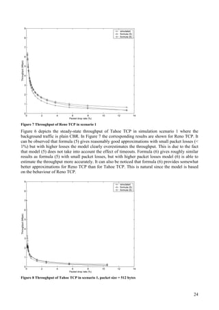
7
where B is the packet size, R is the round trip delay and p is the steady-state packet drop rate.
This model should give reasonably reliable results with small packet losses (< 2%), but with higher
loss rates it can considerably overestimate TCP’s throughput. Also, the equations derived do not
take into account the effect of retransmit timers. Basically, TCP can detect packet loss either by
receiving “triple-duplicate” acknowledgements (four ACKs having the same sequence number), or
via time-outs. In this model it is assumed that packet loss is observed solely by triple duplicate
ACKs.
2.2.2. Complex model
A good model for predicting TCP throughput should capture both the time-out and “triple-
duplicate” ACK loss indications and provide fairly accurate estimates also with higher packet
losses. A more complex model presented in [PFTK98] takes time-outs into account and is
applicable for broader range of loss rates. In [PFTK98] the following approximation of TCP’s
throughput, B(p):
(6)
( )÷
÷
÷
÷
÷
ø
ö
ç
ç
ç
ç
ç
è
æ
+÷
÷
ø
ö
ç
ç
è
æ
+
≈
2
0
max
321
8
3
3,1min
3
2
1
,min)(
pp
bp
T
bp
RTT
RTT
W
pB ,
where Wmax is the receiver’s advertised window and thus the upper bound for the congestion
window, RTT is the round trip time, p the loss indication rate, T0 TCP’s average retransmission
time-out value and b the number of packets that are acknowledged by each ACK. In the
denominator, the first term is due to triple-duplicate acks, and the second term models the timeouts.
With larger loss rates the second term dominates.
3. Ns2
3.1. Installing and using ns2
Ns2 can be built and run both under Unix and Windows. Instructions on how to install ns2 on
Windows can be found at: http://www.isi.edu/nsnam/ns/ns-win32-build.html. However, the
installation may be smoother under Unix. You just have to go through the following steps:
Installation:
• Install a fresh ns-allinone package in some directory. Different versions of ns-allinone
package can be downloaded from: http://www.isi.edu/nsnam/dist/. Select for instance
version 2.1b7a or 2.1b8.
• Once you have downloaded the package, extract the files with the command:
tar -xvf ns-allinone-2.1b7a.tar.
• After this, run ./install in ns-allinone-2.1b7a directory (assuming you are using version
2.1b7a).

8
Using ns2:
Before using ns2 you will have to do the following:
• Copy an example use file (use_example.ns2) from:
/projekti/TEKES/Cost279/results/tcpexercise
• This file contains the required settings for environmental variables. Just modify the directory
names in the file so that they correspond to your environment settings.
Each time you start an ns2 session in a shell, you must type “source use_example.ns2”, which, in
effect, initializes your environment settings. Then, to run your simulation script “myscript.tcl”, just
write:
ns myscript.tcl
Modifying ns2
If you have made some changes in the C++ code, run make in the ns-allinone-2.1b7a/ns-2.1b7a
directory.
3.2. General description
Ns2 is an event driven, object oriented network simulator enabling the simulation of a variety of
local and wide area networks. It implements different network protocols (TCP, UDP), traffic
sources (FTP, web, CBR, Exponential on/off), queue management mechanisms (RED, DropTail),
routing protocols (Dijkstra) etc. Ns2 is written in C++ and Otcl to separate the control and data path
implementations. The simulator supports a class hierarchy in C++ (the compiled hierarchy) and a
corresponding hierarchy within the Otcl interpreter (interpreted hierarchy).
The reason why ns2 uses two languages is that different tasks have different requirements: For
example simulation of protocols requires efficient manipulation of bytes and packet headers making
the run-time speed very important. On the other hand, in network studies where the aim is to vary
some parameters and to quickly examine a number of scenarios the time to change the model and
run it again is more important.
In ns2, C++ is used for detailed protocol implementation and in general for such cases where every
packet of a flow has to be processed. For instance, if you want to implement a new queuing
discipline, then C++ is the language of choice. Otcl, on the other hand, is suitable for configuration
and setup. Otcl runs quite slowly, but it can be changed very quickly making the construction of
simulations easier. In ns2, the compiled C++ objects can be made available to the Otcl interpreter.
In this way, the ready-made C++ objects can be controlled from the OTcl level.
There are quite many understandable tutorials available for new ns-users. By going through, for
example, the following tutorials should give you a rather good view of how to create simple
simulation scenarios with ns2:
http://nile.wpi.edu/NS/

9
http://www.isi.edu/nsnam/ns/tutorial/index.html
The next chapters will summarise and explain the key features of tcl and ns2, but in case you need
more detailed information, the ns-manual and a class hierarchy by Antoine Clerget are worth
reading:
http://www.isi.edu/nsnam/ns/ns-documentation.html
http://www-sop.inria.fr/rodeo/personnel/Antoine.Clerget/ns/ns/ns-current/HIER.html
Other useful ns2 related links, such as archives of ns2 mailing lists, can be found from ns2
homepage:
http://www.isi.edu/nsnam/ns/index.html
3.3. Otcl basics
This chapter introduces the syntax and the basic commands of the Otcl language used by ns2. It is
important that you understand how Otcl works before moving to the chapters handling the creation
of the actual simulation scenario.
3.3.1. Assigning values to variables
In tcl, values can be stored to variables and these values can be further used in commands:
set a 5
set b [expr $a/5]
In the first line, the variable a is assigned the value “5”. In the second line, the result of the
command [expr $a/5], which equals 1, is then used as an argument to another command, which in
turn assigns a value to the variable b. The “$” sign is used to obtain a value contained in a variable
and square brackets are an indication of a command substitution.
3.3.2. Procedures
You can define new procedures with the proc command. The first argument to proc is the name of
the procedure and the second argument contains the list of the argument names to that procedure.
For instance a procedure that calculates the sum of two numbers can be defined as follows:
proc sum {a b} {
expr $a + $b
}
The next procedure calculates the factorial of a number:
proc factorial a {
if {$a <= 1} {
return 1
}

10
#here the procedure is called again
expr $x * [factorial [expr $x-1]]
}
It is also possible to give an empty string as an argument list. However, in this case the variables
that are used by the procedure have to be defined as global. For instance:
proc sum {} {
global a b
expr $a + $b
}
3.3.3. Files and lists
In tcl, a file can be opened for reading with the command:
set testfile [open test.dat r]
The first line of the file can be stored to a list with a command:
gets $testfile list
Now it is possible to obtain the elements of the list with commands (numbering of elements starts
from 0) :
set first [lindex $list 0]
set second [lindex $list 1]
Similarly, a file can be written with a puts command:
set testfile [open test.dat w]
puts $testfile “testi”
3.3.4. Calling subprocesses
The command exec creates a subprocess and waits for it to complete. The use of exec is similar to
giving a command line to a shell program. For instance, to remove a file:
exec rm $testfile
The exec command is particularly useful when one wants to call a tcl-script from within another tcl-
script. For instance, in order to run the tcl-script example.tcl multiple times with the value of the
parameter “test” ranging from 1 to 10, one can type the following lines to another tcl-script:
for {set ind 1} {$ind <= 10} {incr ind} {
set test $ind
exec ns example.tcl test
}

11
3.4. Creating the topology
To be able to run a simulation scenario, a network topology must first be created. In ns2, the
topology consists of a collection of nodes and links.
Before the topology can be set up, a new simulator object must be created at the beginning of the
script with the command:
set ns [new Simulator]
The simulator object has member functions that enable creating the nodes and the links, connecting
agents etc. All these basic functions can be found from the class Simulator. When using functions
belonging to this class, the command begins with “$ns”, since ns was defined to be a handle to the
Simulator object.
3.4.1. Nodes
New node objects can be created with the command
set n0 [$ns node]
set n1 [$ns node]
set n2 [$ns node]
set n3 [$ns node]
The member function of the Simulator class, called “node” creates four nodes and assigns them to
the handles n0, n1, n2 and n3. These handles can later be used when referring to the nodes. If the
node is not a router but an end system, traffic agents (TCP, UDP etc.) and traffic sources (FTP,
CBR etc.) must be set up, i.e, sources need to be attached to the agents and the agents to the nodes,
respectively.
3.4.2. Agents, applications and traffic sources
The most common agents used in ns2 are UDP and TCP agents. In case of a TCP agent, several
types are available. The most common agent types are:
• Agent/TCP – a Tahoe TCP sender
• Agent/TCP/Reno – a Reno TCP sender
• Agent/TCP/Sack1 – TCP with selective acknowledgement
The most common applications and traffic sources provided by ns2 are:
• Application/FTP – produces bulk data that TCP will send
• Application/Traffic/CBR – generates packets with a constant bit rate
• Application/Traffic/Exponential – during off-periods, no traffic is sent. During on-periods,
packets are generated with a constant rate. The length of both on and off-periods is
exponentially distributed.
• Application/Traffic/Trace – Traffic is generated from a trace file, where the sizes and
interarrival times of the packets are defined.

12
In addition to these ready-made applications, it is possible to generate traffic by using the methods
provided by the class Agent. For example, if one wants to send data over UDP, the method
send(int nbytes)
can be used at the tcl-level provided that the udp-agent is first configured and attached to some
node.
Below is a complete example of how to create a CBR traffic source using UDP as transport protocol
and attach it to node n0:
set udp0 [new Agent/UDP]
$ns attach-agent $n0 $udp0
set cbr0 [new Application/Traffic/CBR]
$cbr0 attach-agent $udp0
$cbr0 set packet_size_ 1000
$udp0 set packet_size_ 1000
$cbr0 set rate_ 1000000
An FTP application using TCP as a transport protocol can be created and attached to node n1 in
much the same way:
set tcp1 [new Agent/TCP]
$ns attach-agent $n1 $tcp1
set ftp1 [new Application/FTP]
$ftp1 attach-agent $tcp1
$tcp1 set packet_size_ 1000
The UDP and TCP classes are both child-classes of the class Agent. With the expressions [new
Agent/TCP] and [new Agent/UDP] the properties of these classes can be combined to the new
objects udp0 and tcp1. These objects are then attached to nodes n0 and n1. Next, the application is
defined and attached to the transport protocol. Finally, the configuration parameters of the traffic
source are set. In case of CBR, the traffic can be defined by parameters rate_ (or equivalently
interval_, determining the interarrival time of the packets), packetSize_ and random_ . With the
random_ parameter it is possible to add some randomness in the interarrival times of the packets.
The default value is 0, meaning that no randomness is added.
3.4.3. Traffic Sinks
If the information flows are to be terminated without processing, the udp and tcp sources have to be
connected with traffic sinks. A TCP sink is defined in the class Agent/TCPSink and an UDP sink is
defined in the class Agent/Null.
A UDP sink can be attached to n2 and connected with udp0 in the following way:
set null [new Agent/Null]
$ns attach-agent $n2 $null
$ns connect $udp0 $null

13
A standard TCP sink that creates one acknowledgement per a received packet can be attached to n3
and connected with tcp1 with the commands:
set sink [new Agent/Sink]
$ns attach-agent $n3 $sink
$ns connect $tcp1 $sink
There is also a shorter way to define connections between a source and the destination with the
command:
$ns create-connection <srctype> <src> <dsttype> <dst> <pktclass>
For example, to create a standard TCP connection between n1 and n3 with a class ID of 1:
$ns create-connection TCP $n1 TCPSink $n3 1
One can very easily create several tcp-connections by using this command inside a for-loop.
3.4.4. Links
Links are required to complete the topology. In ns2, the output queue of a node is implemented as
part of the link, so when creating links the user also has to define the queue-type.
Figure 2 Link in ns2
Figure 2 shows the construction of a simplex link in ns2. If a duplex-link is created, two simplex-
links will be created, one for each direction. In the link, packet is first enqueued at the queue. After
this, it is either dropped, passed to the Null Agent and freed there, or dequeued and passed to the
Delay object which simulates the link delay. Finally, the TTL (time to live) value is calculated and
updated.
Links can be created with the following command:
$ns duplex/simplex-link endpoint1 endpoint2 bandwidth delay queue-type
n1 n3
Queue Delay TTL
Agent/Null
Simplex Link

14
For example, to create a duplex-link with DropTail queue management between n0 and n2:
$ns duplex-link $n0 $n2 15Mb 10ms DropTail
Creating a simplex-link with RED queue management between n1 and n3:
$ns simplex-link $n1 $n3 10Mb 5ms RED
The values for bandwidth can be given as a pure number or by using qualifiers k (kilo), M (mega), b
(bit) and B (byte). The delay can also be expressed in the same manner, by using m (milli) and u
(mikro) as qualifiers.
There are several queue management algorithms implemented in ns2, but in this exercise only
DropTail and RED will be needed.
3.5. Tracing and monitoring
In order to be able to calculate the results from the simulations, the data has to be collected
somehow. Ns2 supports two primary monitoring capabilities: traces and monitors. The traces enable
recording of packets whenever an event such as packet drop or arrival occurs in a queue or a link.
The monitors provide a means for collecting quantities, such as number of packet drops or number
of arrived packets in the queue. The monitor can be used to collect these quantities for all packets or
just for a specified flow (a flow monitor)
3.5.1. Traces
All events from the simulation can be recorded to a file with the following commands:
set trace_all [open all.dat w]
$ns trace-all $trace_all
$ns flush-trace
close $trace_all
First, the output file is opened and a handle is attached to it. Then the events are recorded to the file
specified by the handle. Finally, at the end of the simulation the trace buffer has to be flushed and
the file has to be closed. This is usually done with a separate finish procedure.
If links are created after these commands, additional objects for tracing (EnqT, DeqT, DrpT and
RecvT) will be inserted into them.
Figure 3 Link in ns2 when tracing is enabled
Queue Delay TTL
Agent/Null
EnqT DeqT
DrpT
RecvT

15
These new objects will then write to a trace file whenever they receive a packet. The format of the
trace file is following:
+ 1.84375 0 2 cbr 210 ------- 0 0.0 3.1 225 610
- 1.84375 0 2 cbr 210 ------- 0 0.0 3.1 225 610
r 1.84471 2 1 cbr 210 ------- 1 3.0 1.0 195 600
r 1.84566 2 0 ack 40 ------- 2 3.2 0.1 82 602
+ 1.84566 0 2 tcp 1000 ------- 2 0.1 3.2 102 611
- 1.84566 0 2 tcp 1000 ------- 2 0.1 3.2 102 611
+ : enqueue
- : dequeue
d : drop
r : receive
The fields in the trace file are: type of the event, simulation time when the event occurred, source
and destination nodes, packet type (protocol, action or traffic source), packet size, flags, flow id,
source and destination addresses, sequence number and packet id.
In addition to tracing all events of the simulation, it is also possible to create a trace object between
a particular source and a destination with the command:
$ns create-trace type file src dest
where the type can be, for instance,
• Enque – a packet arrival (for instance at a queue)
• Deque – a packet departure (for instance at a queue)
• Drop – packet drop
• Recv – packet receive at the destination
Tracing all events from a simulation to a specific file and then calculating the desired quantities
from this file for instance by using perl or awk and Matlab is an easy way and suitable when the
topology is relatively simple and the number of sources is limited. However, with complex
topologies and many sources this way of collecting data can become too slow. The trace files will
also consume a significant amount of disk space.
3.5.2. Monitors
With a queue monitor it is possible to track the statistics of arrivals, departures and drops in either
bytes or packets. Optionally the queue monitor can also keep an integral of the queue size over
time.
For instance, if there is a link between nodes n0 and n1, the queue monitor can be set up as follows:
set qmon0 [$ns monitor-queue $n0 $n1]
The packet arrivals and byte drops can be tracked with the commands:
set parr [$qmon0 set parrivals_]
set bdrop [$qmon0 set bdrops_]

16
Notice that besides assigning a value to a variable the set command can also be used to get the value
of a variable. For example here the set command is used to get the value of the variable “parrivals”
defined in the queue monitor class.
A flow monitor is similar to the queue monitor but it keeps track of the statistics for a flow rather
than for aggregated traffic. A classifier first determines which flow the packet belongs to and then
passes the packet to the flow monitor.
The flowmonitor can be created and attached to a particular link with the commands:
set fmon [$ns makeflowmon Fid]
$ns attach-fmon [$ns link $n1 $n3] $fmon
Notice that since these commands are related to the creation of the flow-monitor, the commands are
defined in the Simulator class, not in the Flowmonitor class. The variables and commands in the
Flowmonitor class can be used after the monitor is created and attached to a link. For instance, to
dump the contents of the flowmonitor (all flows):
$fmon dump
If you want to track the statistics for a particular flow, a classifier must be defined so that it selects
the flow based on its flow id, which could be for instance 1:
set fclassifier [$fmon classifier]
set flow [$fclassifier lookup auto 0 0 1]
In this exercise all relevant data concerning packet arrivals, departures and drops should be obtained
by using monitors. If you want to use traces, then at least do not trace all events of the simulation,
since it would be highly unnecessary. However, it is still recommended to use the monitors, since
with the monitors you will directly get the total amount of events during a specified time interval,
whereas with traces you will have to parse the output file to get these quantities.
3.6. Controlling the simulation
After the simulation topology is created, agents are configured etc., the start and stop of the
simulation and other events have to be scheduled.
The simulation can be started and stopped with the commands
$ns at $simtime “finish”
$ns run
The first command schedules the procedure finish at the end of the simulation, and the second
command actually starts the simulation. The finish procedure has to be defined to flush the trace
buffer, close the trace files and terminate the program with the exit routine. It can optionally start
NAM (a graphical network animator), post process information and plot this information.
The finish procedure has to contain at least the following elements:

17
proc finish {} {
global ns trace_all
$ns flush-trace
close $trace_all
exit 0
}
Other events, such as the starting or stopping times of the clients can be scheduled in the following
way:
$ns at 0.0 “cbr0 start”
$ns at 50.0 “ftp1start”
$ns at $simtime “cbr0 stop”
$ns at $simtime “ftp1 stop”
If you have defined your own procedures, you can also schedule the procedure to start for example
every 5 seconds in the following way:
proc example {} {
global ns
set interval 5
….
…
$ns at [expr $now + $interval] “example”
}
3.7. Modifying the C++ code
When calculating the throughput according to (6) you will need the time average of TCP’s
retransmission timeout, which is defined based on the estimated RTT. This means that you will
have to be able to trace the current time and the current values of the timeout at that time into some
file, in order to be able to calculate the time average. In ns2 it is possible to trace for example the
value of congestion window to a file with commands:
set f [open cwnd.dat w]
$tcp trace cwnd_
$tcp attach $f
The variable cwnd_ is defined in the C++ code as type TracedInt and it is bounded to the
corresponding Tcl variable making it possible to access and trace cwnd_ at the tcl level. However,
the timeout value is currently visible only at the C++ level. Of course you could get the value of
timeout by adding “printf” commands to the C++ code but a much more elegant way is to define the
timeout variable to be traceable, so that the values can simply be traced at the tcl-level with the
command:
$tcp trace rto_

18
n0 n2n1
3 Mbps
1 ms
5 Mbps
15 ms
The following steps are required in order to be able to trace the timeout value:
In tcp.cc:
• Bind the timeout variable to a variable in the tcl class. The binding allows you to access the
timeout variable also at the tcl level. Furthermore, it ensures that the values of the C++
variable and the corresponding tcl-level variable are always consistent.
• Modify the method TcpAgent::traceVar(TracedVar* v) , which prints out the variable
that you want to trace. It will be helpful to see how the variables cwnd and rtt are handled,
the timeout value can be printed in a similar format.
In tcp.h:
• Change the type of timeout variable to TracedDouble instead of double.
In ns-default.tcl (this file contains the default values of all the tcl variables):
• Set the value of timeout to 0.
After the changes, recompile.
Before running your tcl-script, you will also have to change the value of the tcpTick_ variable in
order to be able to trace the timeout values more accurately. This can be done with a command:
$tcp set tcpTick_ 0.001
3.8. Simple ns2 example
To give you a better idea of how these pieces can be put together, a very simple example script is
given here. The script in itself does not do anything meaningful, the purpose is just to show you
how to construct a simulation.
The script first creates the topology shown in Figure 4 and then adds one CBR traffic source using
UDP as transport protocol and records all the events of the simulation to a trace file.
Figure 4 Example simulation topology

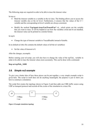
19
The example script:
#Creation of the simulator object
set ns [new Simulator]
#Enabling tracing of all events of the simulation
set f [open out.all w]
$ns trace-all $f
#Defining a finish procedure
proc finish {} {
global ns f
$ns flush-trace
close $f
exit0
}
#Creation of the nodes
set n0 [$ns node]
set n1 [$ns node]
set n2 [$ns node]
#Creation of the links
#Creation of a cbr-connection using UDP
set udp0 [new Agent/UDP]
$ns attach-agent $n0 $udp0
set cbr0 [new Application/Traffic/CBR]
$cbr0 attach-agent $udp0
$cbr0 set packet_size_ 1000
$udp0 set packet_size_ 1000
$cbr0 set rate_ 1000000
$udp0 set class_ 0
set null0 [new Agent/Null]
$ns attach-agent $n2 $null0
$ns connect $udp0 $null0
#Scheduling the events
$ns at 0.0 “$cbr0 start”
$ns at $simtime “$cbr0 stop”
$ns at $simtime “finish”
$ns run

20
S DR
100 Mbps
1 ms
10 Mbps
29 msRED
4. Simulation study
4.1. Description of the problem
The purpose of this study is to verify formulas (5) and (6) for TCP’s steady-state throughput with a
proper simulation setting. In [PFTK98] formula (6) has been verified empirically by analysing
measurement data collected from 37 TCP connections. The following quantities have been
calculated from the measurement traces: number of packets sent, number of loss indications
(timeout or triple duplicate ack), average roundtrip time and average duration of a timeout. The
approximate value of packet loss has been determined by dividing the total number of loss
indications by the total amount of packets sent.
Floyd et al. have verified formula (5) in [F99] by simulations. They have used a simple simulation
scenario where one UDP and one TCP connection share a bottleneck link. The packet drop rate has
been modified by changing the sending rate of the UDP source.
The simulation setting in this study follows quite closely the setting in [F99]. However, in [F99] the
simulations have been performed only in a case when the background traffic is plain CBR. In this
study, the simulations are performed with three slightly different simulation scenarios by using the
topology shown in Figure 5. This topology naturally does not represent a realistic path through the
Internet, but it is sufficient for this particular experiment.
Figure 5 Simulation topology (S = sources, R = router, D = destination)
TCP’s throughput is explored with the following scenarios:
1. Two competing connections: one TCP sender and one UDP sender that share the bottleneck
link. The packet loss experienced by the TCP sender is modified by changing the sending
rate of the UDP flow. FTP application is used over TCP and CBR traffic over UDP (i.e., the
background traffic is deterministic).
2. Two competing connections as above, but now the interarrival times of the UDP sender are
exponentially distributed. The packet loss is modified by changing the average interarrival
time of the UDP packets.
3. A homogeneous TCP population: The packet loss is modified by increasing the number of
TCP sources. Since the TCP sources have same window sizes and same RTT’s, the
throughput of one TCP sender should equal the throughput of the aggregate divided by the
number of TCP sources.

21
The throughput is calculated in scenario 1 and scenario 2 by measuring the number of
acknowledged packets from the TCP connection. Thus in these cases the throughput corresponds to
the sending rate of the TCP source, excluding retransmissions. In scenario 3, the throughput is
calculated from the total amount of packets that leave the queue in the bottleneck link. In addition,
the following quantities are measured in each simulation scenario: number of packets sent, number
of packets lost, average roundtrip time and average duration of a timeout. The number of lost
packets contains only the packets dropped from the TCP connection, or from the TCP aggregate in
scenario 3.
In formulas (5) and (6) the sending rate depends not only on the packet drop rate but also on the
packet size and the round trip time of the connection. Furthermore, the type of the TCP agent
(Tahoe, Reno, Sack) affects on how well the formulas are able to predict the throughput. For
example, formula (6) is derived based on the behaviour of a Reno TCP sender and it will probably
not be as accurate with a Tahoe TCP sender. In this study all three simulation scenarios are
performed with both Tahoe TCP and Reno TCP. Furthermore, experiments on changing the value
of packet size and RTT are made.
4.2. Simulation design considerations
It should be noticed that in this study both the value of the RTT and the timeout correspond to the
values measured by the TCP connection. The values of these variables are traced during the
simulation and finally a time average for RTT and timeout is calculated based on the traces. In
[F99], for example, the value of RTT is not measured but instead, the results are calculated in each
simulation by using a fixed RTT (i.e., 0.06s). In this case, the RTT actually corresponds to the
smallest possible RTT and thus the value given by formula (5) represents an absolute upper bound
for the throughput.
In order to get a proper estimate for the steady-state packet drop rate and throughput, the simulation
time has to be long enough. Furthermore, the transient phase at the beginning of the simulation has
to be removed. In this study, a simulation time of 250 seconds is used and in addition, the collection
of data is started after 50 seconds from the beginning of the simulation. It is shown in chapter 4.3
that with a simulation time of 250 seconds and a transient phase of 50 seconds the estimate for the
steady-state packet drop rate and for the throughput is reasonably accurate.

22
4.2.1. Simulation parameters
The following parameters are used in the configuration:
• Access-link bandwidth – 100 Mbps
• Bottleneck-link bandwidth – 10 Mbps
• Access-link delay – 1 ms
• Bottleneck-link delay – 29 ms
• Queue limits: 100
• TCP type – Tahoe or Reno TCP
• TCP’s maximum window size – 100
• Packet size – 1460 or 512 (in bytes)
• Queue management – RED queue management is used in the bottleneck link and DropTail
in the access link. The value of the parameter Tmax is set to 20, other parameters are set to
the default values defined in ns-default.tcl.
• Starting times of the TCP sources – in case of homogeneous TCP population, the starting
times of the sources are evenly distributed in the interval 0s – 1s. The number of TCP
sources is varied between 1 and 45.
4.3. Numerical results
After each simulation, the actual average throughput of the TCP flow (based on the simulation data)
as well as the throughput according to (5) and (6) is calculated. Finally, the results from different
simulations are plotted as a function of packet loss so that each graph shows the results for a
particular simulation scenario. One point in each graph represents a simulation of 250 seconds. The
points differ only in the sending rate of the UDP flow or in the number of TCP flows in case of a
homogeneous TCP population. All the graphs are plotted using the same scale so that it is easier to
compare the results from different scenarios.
In the graphs only the average results for packet drop rates and throughputs are shown. This is
justified by an observation that with a simulation time of 250 seconds and a transient phase of 50
seconds the standard deviation of the packet drop rate and throughput is rather negligible. The
following tables show the average and standard deviation for the packet drop rate, simulated
throughput and the throughput according to formula (5) and (6) in simulation scenarios 2 and 3
when 10 replications is used. The results are presented in a case where the packet loss is small
(around 1 %) and when the packet loss is large (around 10 %). In simulation scenario 1 the
background traffic is deterministic so that it can be assumed that the standard deviation would be
even smaller in this case.
Average Standard deviation
Packet drop rate 0,0101 0,0002
Throughput (Mbps) 1,8865 0,0120
Formula (5) (Mbps) 2,1482 0,0237
Formula (6) (Mbps) 2,0847 0,0246
Table 1 Scenario 2, small packet loss

23
Formula (5) (Mbps) 0,6092 0,0098
Formula (6) (Mbps) 0,3498 0,0159
Table 2 Scenario 2, large packet loss
Formula (5) (Mbps) 1,7011 0,0043
Formula (6) (Mbps) 1,6238 0,0046
Table 3 Scenario 3, small packet loss
Formula (5) (Mbps) 0,5540 0,0025
Formula (6) (Mbps) 0,2593 0,0135
Table 4 Scenario3, large packet loss
0 2 4 6 8 10 12 14
0
1
2
3
4
5
6
7
8
9
Packet drop rate (%)
Throughput(Mbps)
simulated
formula (5)
formula (6)
Figure 6 Throughput of Tahoe TCP in scenario 1

24
0 2 4 6 8 10 12 14
0
1
2
3
4
5
6
7
8
9
Throughput(Mbps)
simulated
formula (5)
formula (6)
Figure 7 Throughput of Reno TCP in scenario 1
Figure 6 depicts the steady-state throughput of Tahoe TCP in simulation scenario 1 where the
background traffic is plain CBR. In Figure 7 the corresponding results are shown for Reno TCP. It
can be observed that formula (5) gives reasonably good approximations with small packet losses (<
1%) but with higher losses the model clearly overestimates the throughput. This is due to the fact
that model (5) does not take into account the effect of timeouts. Formula (6) gives roughly similar
results as formula (5) with small packet losses, but with higher packet losses model (6) is able to
estimate the throughput more accurately. It can also be noticed that formula (6) provides somewhat
better approximations for Reno TCP than for Tahoe TCP. This is natural since the model is based
on the behaviour of Reno TCP.
0 2 4 6 8 10 12 14
0
1
2
3
4
5
6
7
8
9
Throughput(Mbps)
simulated
formula (5)
formula (6)
Figure 8 Throughput of Tahoe TCP in scenario 1, packet size = 512 bytes

25
Figure 8 shows the results for Tahoe TCP in scenario 1 when the packet size is 512 bytes. It seems
that with this packet size also formula (5) is able to predict the throughput reasonably well, even
with higher packet losses.
0 2 4 6 8 10 12 14
0
1
2
3
4
5
6
7
8
9
Throughput(Mbps)
simulated
formula (5)
formula (6)
0 2 4 6 8 10 12 14
0
1
2
3
4
5
6
7
8
9
Throughput(Mbps)
simulated
formula (5)
formula (6)
Figure 9 and Figure 10 present the steady-state throughput of Tahoe and Reno TCP in simulation
scenario 2 where the interarrival times of the UDP source are exponentially distributed. It seems
that also in this scenario formula (5) overestimates the throughput whereas formula (6) is able to

26
approximate the throughput more accurately. In fact, from Figure 10 it can be observed that when
Reno TCP is used the results from formula (6) are very close to the simulated results.
It seems that in scenario 2 at least formula (6) is able to predict the throughput more accurately than
in scenario 1 where the traffic was plain CBR. This difference can be explained by the fact that the
applicability of the assumptions in models (5) and (6) depends on the traffic process of the UDP
source.
0 2 4 6 8 10 12 14
0
1
2
3
4
5
6
7
8
9
Throughput(Mbps)
simulated
formula (5)
formula (6)
0 2 4 6 8 10 12 14
0
1
2
3
4
5
6
7
8
9
Throughput(Mbps)
simulated
formula (5)
formula (6)

27
Figure 11 and Figure 12 present the steady-state throughput of Tahoe and Reno TCP in simulation
scenario 3 where a homogeneous TCP population is used. As in previous simulation scenarios, it
can be observed that models (5) and (6) give very similar results with small packet losses but the
throughput approximated by formula (6) decreases faster with higher packet losses providing better
estimates than formula (5). It should be noted that the actual average throughput of one TCP source
is calculated by dividing the throughput of the aggregate by a number of TCP sources. Although the
bandwidth should be divided equally since the window sizes and RTTs are same for every source,
this may not always be the case. Thus the throughput of an individual TCP source might differ from
its fair share.
0 2 4 6 8 10 12 14
0
1
2
3
4
5
6
7
8
9
Throughput(Mbps)
simulated
formula (5)
formula (6)
Figure 13 Throughput of Reno TCP in scenario 3, rtt = 0.03s
0 2 4 6 8 10 12 14
0
1
2
3
4
5
6
7
8
9
Throughput(Mbps)
simulated
formula (5)
formula (6)
Figure 14 Throughput of Reno TCP in scenario 3, rtt = 0.09s

28
Figure 13 and Figure 14 present the steady-state throughput of Tahoe TCP in simulation scenario 3
with two different RTTs, 0.03 seconds and 0.09 seconds. With an RTT of 0.03 seconds the
simulated throughput as well as the throughput approximated by formula (5) and (6) is naturally
higher than with an RTT of 0.09 seconds.
References
[F99] S.Floyd, “Promoting the Use of End-toEnd Congestion Control in the Internet”, IEEE/ACM
TRANSACTIONS ON NETWORKING, VOL. 7, NO.4, AUGUST 1999.
[PFTK98] J.Padhye, V.Firoiu, D.Towsley, J.Kurose, “Modeling TCP Throughput: A Simple Model
and its Empirical Validation”, In Proc. ACM SIGCOMM ’98 1998.
[APS99] M.Allman, V.Paxson, W.R.Stevens, “TCP Congestion Control”, STD1, RFC 2581, April
1999.

Tcp performance simulationsusingns2

Recommended

Recommended

More Related Content

What's hot

What's hot (20)

Similar to Tcp performance simulationsusingns2

Similar to Tcp performance simulationsusingns2 (20)

Recently uploaded

Recently uploaded (20)

Tcp performance simulationsusingns2