Validation of time domain spectral element-based wave finite element method for 1D axial periodic structures

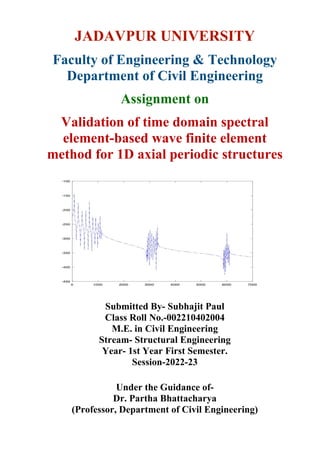
1. JADAVPUR UNIVERSITY
Faculty of Engineering & Technology
Department of Civil Engineering
Assignment on
Validation of time domain spectral
element-based wave finite element
method for 1D axial periodic structures
Submitted By- Subhajit Paul
Class Roll No.-002210402004
M.E. in Civil Engineering
Stream- Structural Engineering
Year- 1st Year First Semester.
Session-2022-23
Under the Guidance of-
Dr. Partha Bhattacharya
(Professor, Department of Civil Engineering)

2. Acknowledgement
I would like to express my gratitude to Dr. Partha Bhattacharya (Professor,
Department of Civil Engineering) for his guidance, academic
encouragement and friendly critique. His attitude and care have helped me
to complete this assignment on time. I would like to thank Mr. Shuvajit
Mukherjee for his advice and cooperation as he helped me to access
information from relevant sources.
I extend my gratitude to Jadavpur University for giving me this
opportunity.
At last but not least gratitude goes to all of my friends who directly or
indirectly helped me to complete this assignment.
Subhajit Paul
M.E. in Civil Engineering
Jadavpur University

3. Abstract
In this work, a time domain spectral element-based wave finite element
method is proposed to analyze periodic structures. Time domain spectral
element-based formulation reduces the total degrees of freedom and also
renders a diagonal mass matrix resulting in substantial reduction in
computation time for the wave finite element method. The formulation is
then considered to obtain the stop band characteristics for a periodic bar
considering geometric as well as material periodicity. The impact of
geometric parameters on the stop bands of 1-D structures is then
investigated in detail. It is shown that the stop bands can be obtained in the
frequency range of interest, and its width can be varied by tuning those
geometric parameters. Also, the effect of material uncertainty is studied in
detail on the stop band characteristics of periodic 1-D structures, and the
same formulation is utilized for Monte Carlo simulations. Results show
that randomness in density influences more the bandwidth of the stop
bands than that of elastic parameters.

4. CONTENTS
1.Introduction 1
1.1.Background 1
2. Longitudinal Waves in Rods 3
2.1. Elementary rod modeling 3
2.1.1. Equation of Motion and Spectral Analysis 4
2.2. Basic Solution for Waves in Rods 6
3. Spectral Element for Rods 8
3.1. Shape Functions 8
3.2. Dynamic Stiffness for Rods 10
3.3. Efficiency of a Spectral Element method over Conventional
method 11
3.3.1. Spectral Element 13
3.3.2. Conventional Element 13
4. Wave finite element 14
4.1. Bloch’s theorem 14
4.2. Finite element analysis of a unit cell 14
4.3. Transfer matrix 16
4.3.1. Eigenvalue and eigenvector of the transfer matrix 16
4.3.2. Generalized eigenvalue analysis 17
4.4. Periodic 1-D analysis 18
5. Time domain spectral element method 19
6. Numerical analysis 21
6.1. Analysis of a 1-D bar 21
6.1.1.Stop bands and parametric analysis of a periodic bar 21
6.1.2. Effect of material uncertainty on stop bands 25
7. Conclusions 28
8. Future scope 29
References 29

5. Validation of time domain spectral element-based wave finite element
method for 1D axial periodic structures
1. Introduction
A periodic structure can be defined as a structure or material which is formed by repetition of an
identical representative element named a unit cell [1]. The repetition can be in the form of
material properties, boundary conditions, geometry, etc. Depending upon the complexity and
dimension of the structure, the complexity and the dimension of a unit cell can vary considerably.
Aerospace structures are very susceptible to transient types of loading which typically contain
considerable high-frequency content. Therefore, the use of periodic structures in the design of
aerospace structures acts as a bandpass filter for a particular wave with undesirable frequency
content. In periodic structures, the stop bands are generated as a consequence of destructive
interference between the incident wave and the reflecting wave due to the change in geometry or
material properties. The wavenumber remains constant in the frequency values corresponding to
the stop bands which indicates zero group speed. Thus, waves of a certain frequency range
cannot propagate through the structure, and undesired vibration can be avoided by proper design.
The stop bands are the main points of interest of periodic structures which motivates the research
on the use of periodic structures for vibration attenuation. The behaviour of the whole structure
can be analyzed by performing an analysis of a unit cell which is the main motivation of periodic
analysis. The periodic analysis is independent of the domain and number of unit cells.
1.1. Background
The first study of periodic structures was done by Newton to describe the propagation of the
sound wave in air using lumped masses and attached massless springs as mentioned by Brillouin
in his book [2]. Thereafter, much work regarding periodic structures was performed in optics and
electromagnetic wave related research. Research in periodic structures from the perspective of
structural wave propagation started back in 1887 when Rayleigh [3] studied a stretched string
with periodically varying density along its length subjected to a transverse harmonic load.
Brillouin [2] and Flochet [4] made major contributions in the field of wave propagation of
periodic structures. Their studies were based on the understanding of wave characteristics of
lattice structures which is in the field of solid-state physics. Two-dimensional engineering
periodic structures composed of rectangular grillage of interconnected uniform beams with both
flexural and torsional stiffness were studied by Heckl [5]. This study was further revised by
Hodges [6] for disordered periodic structures. Mead [1,7] proposed a general theory of wave
propagation in both mono-coupled and multi-coupled periodic systems. The general theory
depicts that the number of waves is twice the minimum number of degrees of freedom at
coupling interfaces and can be decomposed into an equal number of positive and negative
travelling waves. Later, Mead [8] published a review article summarizing his work and that of his
colleagues of the University of Southampton which addresses their enormous contribution to the
field of periodic structures. Lin and McDaniel [9] developed an analytical technique to determine
the frequency response of a 1-D Euler– Bernoulli beam structure. They investigated the transfer
matrix method (TMM) and associated numerical issues in detail. The transfer matrix (TM)
basically relates the state vector of the right and left boundary of a periodic cell. The propagation
constant can be derived from the eigenvalue analysis of TM and the wavenumber can be found
from the propagation constant. The wavenumber derived from the TMM is a complex number.
1

6. Therefore, both the propagating and evanescent part of waves can be found. The transfer matrix
of the periodic systems can be found both analytically and by the finite element method. Several
works are found in literature considering the analytical approach [10,11]. The advantages of
TMM notwithstanding, the transfer matrix can be ill-conditioned. Still, TMM has been used to
solve wave propagation problems across a wide domain such as for smart materials, beams,
plates, piezoelectric patches, functionally graded material, and many others [12–15].
Apart from the transfer matrix method, there are many other methods available in the literature to
calculate the wave propagation characteristics, and researchers have explored them considering
different kinds of periodic structures. The methods are plane wave expansion method (PWE),
extended plane wave expansion method (EPWE), finite difference time domain method (FDTD),
finite element method, spectral element method (SEM), and wave finite element method [16].
Among all the methods mentioned above, the transfer matrix method (TMM) is very popular for
analyzing periodic structures. Researchers used it along with the finite element and spectral
element method to determine band gaps of periodic structures.
In SEM, the dynamic stiffness matrix is formed, and the dynamic response of the structure is
expressed using spectral representations [17]. Compared to conventional finite element, SEM
reduces the computational cost substantially. Motivated by these facts, Lee [18] used SEM with
TMM to analyze periodic structures with an idea to reduce the computation cost for dynamic as
well as wave propagation problems. However, it is often difficult to obtain the exact solution
required to get the dynamic stiffness matrix. The development of the frequency dependent
stiffness matrix is case specific, and to address the difficulties of SEM, researchers came up with
the wave finite element (WFE) method. For complex structures, evaluation of the analytical
transfer matrix is difficult, so the finite element method is integrated to model the unit cell of a
periodic structure. Mace et al.[19] and Houllin et al. [20] had proposed the WFE. Mace et al. [19]
obtained the dispersion relations, and Duhamel et al. [21] calculated the forced vibration
response for periodic structures. In WFE, a section of the waveguide is modeled by conventional
finite elements. One can exploit the commercial FE packages in this part of the problem. The
stiffness and mass matrix are obtained, and the dynamic stiffness matrix of the unit cell is
obtained explicitly. Details of WFE are provided in the work of Duhamel et al. [21]. WFE is
applied to diverse types of problems starting from a homogeneous waveguide, like beam [22],
plate [23], fluid filled pipes [24], and simple periodic structures to complex periodic media [25–
29]. In WFE, a single cell is meshed with finite elements rather than the whole waveguide which
is done in case of the standard finite element approach. In WFE, the computation cost is much
lower than that in the conventional finite element approach, and complex geometries can also be
modeled via WFE. The main motivation of the WFE approach is to reduce the cost of the
periodic analysis and also to utilize the conventional finite elements and exploit finite element
packages which are well developed. However, the minimum wavelength dictates the element
length of the finite element. As per Ichchou [30], the number of elements should be at least 6 to
10 per wavelength to predict the wavenumber properly.
However, suggestions typically vary from problem to problem. Thus, the element length can
have a far more smaller value than for h-fem. Note that p-fem can lead to better results but the
polynomial degrees cannot be increased arbitrarily as the Runge phenomenon causes huge
oscillation near the boundary nodes, thus resulting in erroneous prediction [31]. The time domain
spectral element method (TSEM) also uses higher order polynomials like p-fem but avoids the
Runge phenomenon. The number of degrees of freedom for TSEM is much lower than for
conventional finite elements, and the mass matrix is inherently diagonal. Thus, TSEM based
modeling is explored to model the waveguide for the improvement of WFE. TSEM can be
utilized to solve the micro and macrostructure problems in multiscale modeling [32–34] of
2

7. materials. The atomistic scale and continuum TSEM model can be coupled by non-local
elasticity formulation wherein the scale effects can be introduced in the TSEM model. It also can
be beneficial for solving static and dynamic fracture mechanics problems [35] considering the
phase field method due to its effective properties mentioned earlier.
In this study, a new wave finite element formulation is proposed considering the time domain
spectral element method to analyze the periodic 1-D bar. A considerable amount of reduction in
computation time is achieved with this formulation. A detailed numerical study is then performed
to obtain the stop band characteristics of 1D periodic structures. The effects of different
parameters on the stop bands are also discussed in detail. On the other hand, uncertainty in the
geometric and material parameters is unavoidable as it occurs primarily due to the manufacturing
process, and it also influences the static and dynamic behaviour of the engineering structures. In
case of periodic structures, the position and width of the band gap is sensitive to the material and
the geometric properties of the constitutive cell. Therefore, the uncertainty in these parameters
should be included in the analysis to obtain a realistic design of the band gap in periodic
structures. In this paper, the effect of material uncertainty on the wave propagation characteristics
of 1D periodic structures is obtained. To perform the analysis, Monte Carlo simulation (MCS) is
used considering the developed WFE formulation.
2. Longitudinal Waves in Rods
Rods and struts are important structural elements and form the basis of many truss and grid
frameworks. Because their load bearing capability is axial, then as waveguides they conduct only
longitudinal wave motion.
That begins by using elementary mechanics to obtain the equations of motion of the rod. As it
happens, the waves are governed by the simple wave equation and so many of the results are
easily interpreted. The richness and versatility of the spectral approach is illustrated by
considering such usually complicating factors as viscoelasticity and elastic constraints. Particular
emphasis is placed on the waves interacting with discontinuities such as boundaries and changes
in cross section, as shown in Fig.1.
The basic waves in rods are described by a single mode; coupled thermo elasticity is introduced
here as a first example of handling multi-mode problems where the coupling is between
temperature and displacement (strain).
2.1. Elementary rod modeling
There are various schemes for deriving the equations of motion for structural elements. The
approach taken here is to begin with the simplest available model, and then as the need arises to
append modifications to it. In this way, both the mechanics and the wave phenomena can be
focused on without being unduly hindered by some cumbersome mathematics.
Fig. 1 Segment of rod with loads
3

8. 2.1.1. Equation of Motion and Spectral Analysis
The elementary model considers the rod to be long and slender and assumes it supports only 1D
axial stress as shown in Fig. 1. It further assumes that the lateral contraction (or the Poisson’s
ratio effect) can be neglected.
Following the assumption of only one displacement, u(x), the axial strain is given by
(1)
Let the material behaviour be linear elastic, then the 1D form of Hooke’s law gives the stress as
(2)
E = Young’s Modulus
This stress gives rise to a resultant axial force of
(3)
Let qu(x, t) be the externally applied axial force per unit length. While not essential, we consider
the cross section to be rectangular of depth b and height h. With reference to Fig. 1, the balance
of forces gives
(4)
where ρA is the mass density per unit length of the rod, η is the damping (viscous) per unit
volume, and the super dot indicates a time derivative. If the quantities are very small, then the
equation of motion becomes (after dividing through by x)
(5)
The independent variables are x and t. Substituting for the force in terms of the displacement
gives the equation of motion
(6)
In the special case of uniform properties and no damping, all dependent variables (stress, strain,
etc.) have an equation of the form
(7)
for the homogeneous part. In this case, the waves in the rod are governed by the simple wave
equation and the general solution is that of D’Alembert, given by
(8)
∈XX =
∂u
∂x
σXX = E ∈XX = E
∂u
∂x
F =
∫
σXXdA = EA
∂u
∂x
−F + [F + ∆ F] + qu . ∆ x − ηA ∆ x ¨
u = ρA ∆ x ¨
u
∂F
∂x
= ρ
∂
∂x
(
∂u
∂x
) + ηA
∂u
∂x
− qu
EA
∂
∂x
(
∂u
∂x
) − ρ
∂
∂x
(
∂u
∂x
) = ηA
∂u
∂x
− qu
C2
0
∂2
u
∂x2
−
∂2
u
∂x2
= 0; C0 ≡ EA/ρA
u(x, t) = f(x − C0t) + F(x + C0t)
4

9. This solution does not hold for the general rods of interest in this chapter and therefore is not
pursued any further in its present form. The kernel solutions corresponding to this are obtained
by considering the homogeneous equation
(9)
(10)
This is the basic equation used in the remainder of the chapter. Assume that both the modulus and
the area do not vary with position, then the homogeneous differential equation for the Fourier
coefficients becomes
(11)
This is an ordinary differential equation with constant coefficients—the frequency is considered
as a parameter. Because this equation has constant coefficients, then it has the exponential
solutions e−ikx leading to
(12)
(14)
Where are the undetermined amplitudes at each frequency. When combined with the
time variation, this solution corresponds to two waves: a forward-moving wave and a backward-
moving wave. That is,
(15)
It is understood that all quantities inside the summation could depend on the frequency ω.
The spectrum relation for the undamped case is continuous line; if it is a straight line then-
(16)
The comparison is with FE-generated data using a vibration eigen analysis. To see how this is
accomplished, consider a rod with fixed end conditions. The undamped solution is
= cos(kx) + sin(kx). (17)
where and are real only. The zero displacement BCs give
0 = , 0 = cos(kL) + sin(kL) (18)
d
d x
[EA
∂^
u
∂x
]i2
ω2^
uρA − iω^
uηA = − ^
qu
.
d
d x
[EA
d^
u
d x
] + ω2
ρA^
u − iωηA^
u = − ^
qu
.
EA
d
d x
(
d^
u
d x
) + (ω2
ρA − iωηA)^
u = 0
^
u(x) = ^
Ae−ik1x
+ ^
Be+ik1x
k1 ≡ (ω2
ρA − iωηA)/EA
^
A and ^
B
u(x, t) =
∑
^
Ae−i[k1x−ωt]
+
∑
^
Be+i[k1x+ωt]
k1 = ω ρA/EA
^
u(x) c1 c2
c1 c2
c1 c1 c2
5

10. This leads to the eigen solution c1 = 0, c2 = ? ⇒ sin(kL) = 0. The latter is satisfied when k = nπ/
L. Therefore, the spectrum relation is obtained by counting the number of half-waves and plotting
against frequency. Confirmation is hardly necessary in this case but becomes crucially important
in our later more complex cases, particularly when there are multiple modes present. The FE
results show a slight deviation at the maximum frequency and has to do with the discretization
using elements. We use the FE method in this way quite often and therefore refer to it as FE
spectrum relation.
The undamped spectrum relation gives constant phase and group speeds of
c = ω/k = √EA /ρA = , = dω/dk = √EA/ρA = (19)
2.2. Basic Solution for Waves in Rods
Fig. 2 Free body for the point impact of a rod
Let the end of the rod at x = 0 be subjected to a force history
P (t); then according to the free body of Fig. 2, we have
at x = 0 : F = EA∂u(x, t) /∂x = −P (t). (20)
Let all functions of time have the spectral representation; the boundary condition becomes, in
expanded form,
(21)
This has to be true for all time; hence, the equality must be true on a term-by-term basis giving
(22)
Problems like this impact problem always reduce to establishing the relationships at a particular
n (or frequency ωn); hence, the subscript can usually be omitted (but understood). The condition
at x = 0 now becomes (using the solution and because there is only a forward-moving wave)
(23)
c0 cg c0
EA
d
d x ∑n
^
un(x)eiωnt
= −
∑n
^
Pneiωnt
EA
d^
un
d x
= − ^
Pn
EA{ − ik1
^
A} = − ^
P
⇒ ^
A =
^
P
ik1EA
6

11. The complete solution for the forward-moving wave is therefore
(24)
or (to emphasize the frequency dependence) with every subscript written out explicitly
(25)
Knowing the spectrum of the force history, , the displacement (and, consequently, the stress,
etc.) can be determined at any location x. As is apparent, the disturbance travels at the now
familiar constant speed of = √EA/ρA.
The transfer function, , for this case is
(26)
The transfer function for the velocity, on the contrary, is
(27)
and the amplitude is relatively insensitive to frequency because the damping is usually small.
Consequently, the windowing parameters used for transforming the force are also appropriate for
reconstructing the velocity. Using the subscripts i and r to represent the forward- and backward-
moving waves, respectively, then the other mechanical quantities (at a particular frequency) can
be obtained as
Displacement:
Velocity:
Strain:
Stress: = −ikE = ikEA
Force: = −ikEA = ikEA
giving the following interesting inter-relationships for the undamped case (when k = ω/ )
(28)
(29)
Thus the history profiles of the particle velocity, force, and stress are the same. Notice that a
tensile stress moving forward causes a negative velocity (i.e., the particles move backward).
u(x, t) =
∑
^
P
ik1EA
e−i[k1x−ωt]
u(x, t) =
1
EA ∑n
^
P
ik1n
e−i[k1x−ωnt]
^
P
C0
^
G(x, ω)
^
u = ^
G(x, ω)^
P ; ^
G(x, ω) =
1
ik1EA
e−ik1x
^
Gυ(x, ω) = iω^
G(x, ω) =
ω
(ω2ρA − iωηA)EA
e−ik1x
ui = ^
Ae−i[k1x−ωt]
ur = ^
Be−i[k1x−ωt]
u̇i = iωui u̇r = iωur
ϵi = − ikui ϵr = ikur
σi ui σr ur
Ti ui Tr ur
C0
u̇i = ikC0ui = −
C0
E
σi = −
C0
EA
Fi
u̇r = ikC0ur =
C0
E
σr =
C0
EA
Fr
7

12. Also, note that the convention for the sign of the forces, and , is that of the stress because they
are internal forces.
3. Spectral Element for Rods
The only way to efficiently handle wave propagation problems in structures with complicated
boundaries and discontinuities is to develop a matrix methodology for use on a computer.
Our approach is similar in style to that of the finite element (FE) method but has the very
significant difference that the element stiffness matrix is established in the frequency domain.
This allows the effects of the inertia of the distributed mass to be described exactly. As a
consequence, these spectrally formulated elements describe exactly the wave propagation
dynamics and (in contrast to the conventional element) this means that elements can span all the
way from one joint to another without losing fidelity. Furthermore, the system of equations to be
solved is very small. The approach provides all the advantages of the spectral analysis method
plus the efficiency and organization of the finite element method. The spectral element idea is
generalized through the spectral super-element which is necessary for the accurate description for
the connection between waveguides in a general setting. The spectral super-element also adds
depth to the understanding of periodic structures.
We illustrate the use of the spectral element approach on identification problems as well as
compact analyses of periodic structures.
3.1. Shape Functions
There are a variety of ways to establish a dynamic stiffness relation; in this and the following
sections, we find it more fruitful to approach it via dynamic shape functions. These are
essentially interpolation functions between the element ends, but instead of being simple
polynomials, they are the exact displacement distributions. However, equilibrium is established
from free bodies.
Fig. 3 Nodal loads and degrees of freedom for three spectral elements. (a) Longitudinal, (b) flexural, (c) torsional
Fi Fr
8

13. The general longitudinal displacement for a rod can be written as
(30)
where are constants determined from the BCs on the element. Note that the only restriction
here is that the rod model be a one-mode model; thus it could represent the refined Love model
or a simple rod with elastic constraint; the complexity of the differential equation is embedded in
the spectrum relation (ω).
The displacement end conditions for the two-noded element, shown in Fig. 3a, are
(31)
(32)
(33)
By using matrix form-
(34)
So, we can write-
(35)
Now, we get-
(36)
(37)
Now, finally we get-
^
u(x) = ^
Ae−ik1x
+ ^
Be−ik1(L−x)
^
A, ^
B
k1
^
u(0) = ^
u1 = ^
Ae−ik10
+ ^
Be−ik1[L−0]
= ^
A + ^
Be−ik1L
^
u(L) = ^
u2 = ^
Ae−ik1L
+ ^
Be−ik1(L−L)
= ^
Ae−ik1L
+ ^
B
^
u(x) = ^
Ae−ik1x
+ ^
Be−ik1(L−x)
{
^
u1
^
u2
} = [
1 e−ik1L
e−ik1L
1
]{
^
A
^
B
}
⇒
{
^
A
^
B
} =
1
1 − e−2ik1L
[
1 −e−ik1L
−e−ik1L
1
]{
^
u1
^
u2
}
{^
u} = [e−ik1x
e−ik1(L−x)
]{
^
A
^
B
}
{^
u} = [e−ik1x
e−ik1(L−x)
] 1
1 − e−2ik1L
[
1 −e−ik1L
−e−ik1L
1
]{
^
u1
^
u2
}
{^
u } =
1
1 − e−2ik1L
[e−ik1x
− e−ik1(2L−x)
e−ik1(L−x)
− e−ik1(L+x)
]{
^
u1
^
u2
}
^
u(x) =
e−ik1x
− e−ik1(2L−x)
1 − e−2ik1L
^
u1 +
e−ik1(L−x)
− e−ik1(L+x)
1 − e−2ik1L
^
u2
9

14. (38)
The significance of the shape functions is that the complete description of the element is captured
in the two nodal DoFs . That is, how the forces and other quantities are obtained by
differentiation of the displacements, now because the shape function is predetermined for a
particular structural element, we see that this formulation reduces the unknowns to just the nodal
values.
Because the spectral element can be very long then the ability to compute the response between
nodes is necessary. This can be done conveniently using the shape function and the nodal values.
Thus, the displacements and member forces are obtained simply as
(39)
where the differentiations are easily performed in advance. If required, EA can be replaced with
its frequency dependent counterpart to account for viscoelasticity, say. Now consider the
throw-off element. Because there are no reflections, the term is omitted. We replace the
coefficient with nodal information by using the end condition that
(40)
where a semi-infinite rod can therefore be written as 1 is the single nodal displacement. The
displacement at an arbitrary point in a semi-infinite rod can there fore be written as
(41)
The shape function (x) is frequency dependent and is complex even in the simple rod case with
no damping.
3.2. Dynamic Stiffness for Rods
The member loads at each end of the rod are related to the displacements by
(42)
(43)
The dynamic stiffness of the two noded element can now be written in the matrix form-
⇒ ^
u(x) = ^
g1
(x)^
u1 + ^
g2
(x)^
u2
^
u1, ^
u2
^
F(x) = EA[^
g′

1
(x)^
u1 + ^
g′

2
(x)^
u2
^
EA
^
B
^
A
^
u(0) ≡ ^
u1
^
u1
^
u(x) = ^
g1
(x)^
u1; ^
g1
(x) = [e−ik1x]
^
g1
^
F1 = − ^
F(0) = − ^
EA[^
g′

1
(0)^
u1 + ^
g′

2
(0)^
u2]
^
F2 = ^
F(L) = ^
EA[^
g′

1
(L)^
u1 + ^
g′

2
(L)^
u2]
{
^
F1
^
F2
} = EA[
−^
g′

1
(0) −^
g′

2
(0)
^
g′

1
(L) ^
g′

2
(L)
]{
^
u1
^
u2
}
10

15. ]
]
(44)
So,
Where, [ ] is frequency dependent dynamic element stiffness for the rod.
It is symmetric and real. This can be confirmed by expanding to trigonometric expression-
(45)
3.3. Efficiency of a Spectral Element method over Conventional method
In finite element method-
Element stiffness matrix for rod is given by ;
(46)
(47)
Mass matrix of rod-
The kinetic energy of a general system of concentrated masses are related to the mass and
velocities by;
(48)
The actual kinetic energy is obtained using function of displacement and is,
=
EA
1 − e−2ik1L
[
ik1(1 + e−i2k1L
) −2ik1e−ik1L
−2ik1e−ik1L
ik1(1 + e−i2k1L
)
]{
^
u1
^
u2
}
=
EA . ik1
1 − e−2ik1L
[
(1 + e−i2k1L
) −2e−ik1L
−2e−ik1L
(1 + e−i2k1L
)
{
^
u1
^
u2
}
⇒ {
^
F1
^
F2
} =
EA
L
ik1L
1 − e−2ik1L
[
(1 + e−i2k1L
) −2e−ik1L
−2e−ik1L
(1 + e−i2k1L
)
{
^
u1
^
u2
}
⇒ {
^
F1
^
F2
} = [
^
k11
^
k12
^
k21
^
k22
]{
^
u1
^
u2
}
{^
F} = [
^
K]{^
u}
^
K
{
^
F1
^
F2
} =
EA
L
k1L
Sin(k1L)
[
Cos k1L −1
−1 Cos k1L
]{
^
u1
^
u2
}
[^
K] =
EA
L
[
1 −1
−1 1
]
{
F1
F2
} =
EA
L
[
1 −1
−1 1
]{
u1
u2
}
T =
1
2 ∑i ∑j
mij
^
ui
^
uj Or, mij =
∂2T
∂ui ∂uj
T =
1
2 ∫
L
0
ρA[ ˙
u]
2
dx =
1
2
ρA
∫
L
0
[(1 −
x
L
)u̇1 +
x
L
u̇2]
11

16. 2 + 2}. (49)
Using the above relation gives the equivalent mass matrix by differentiation as
[m]= (50)
The equivalent inertia forces can therefore be written in matrix form as-
(51)
Assembling both elastic and inertia forces give-
{F}={F}+{F’} (52)
[ ]{u}+[m]{ }={F} (53)
For a dynamic problem when excitation force is harmonic;
{F}={ } (54)
Then the response is also harmonic, given by-
{u}={ } (55)
Substituting this into differential equation gives-
[ ]{ } - 2[m]{ } ={ }
2[m]]{ }={ }. (56)
Now;
(57)
It is worth nothing that this equation is recovered exactly in the limit as (and hence k1) goes to
zero.
The stiffness relation for the throw off element is simply-
{ }=EA[I ]{ } (58)
Now, put
⇒ T =
1
2
ρAL{
1
3
u̇1
1
3
u̇1u̇2 +
1
3
u̇2
ρAL
6
[
2 1
1 2
]
{
F′

1
F′

2
} =
ρAL
6
[
2 1
1 2
]{
ü1
ü2
}
^
k ü
^
F eiωt
^
u eiωt
^
k ^
u eiωt
ω ^
u eiωt ^
F eiωt
⇒ [[^
k] − ω ^
u ^
F
{
^
F1
^
F2
} = (
EA
L
[
1 −1
−1 1
] −
ρALω2
6
[
2 1
1 2
]){
^
u1
^
u2
}
ω
^
F1 k1
^
u1
ξ = ω ρA/EA ∗ L = kL
12

17. Then;
(59)
3.3.1. Spectral Element
(60)
When; =0, coskL=0, kL=1.57
3.3.2. Conventional Element
(61)
When;
k11=0; =0, =√3, kL=1.73 [ =kL]
Fig. 4 Spectral element stiffness behaviour Comparison with conventional element at low frequency.
{
^
F1
^
F2
} = (
EA
L
[
1 −1
−1 1
] −
ρALω2
6
[
2 1
1 2
]){
^
u1
^
u2
}
⇒ {
^
F1
^
F2
} =
EA
L
([
1 −1
−1 1
] −
ρAL2
ω2
EA
[
1
3
1
6
1
6
1
3
]){
^
u1
^
u2
}
⇒ {
^
F1
^
F2
} =
EA
L
[
(1 − 1
3
ξ2
) −(1 + 1
6
ξ2
)
−(1 + 1
6
ξ2
) (1 − 1
3
ξ2
)
]{
^
u1
^
u2
}
{
^
F1
^
F2
} =
EA
L
kL
sinkL
[
coskL −1
−1 coskL
]{
^
u1
^
u2
}
k11
{
^
F1
^
F2
} =
EA
L
[
(1 − 1
3
ξ2
) −(1 + 1
6
ξ2
)
−(1 + 1
6
ξ2
) (1 − 1
3
ξ2
)
]{
^
u1
^
u2
}
(1 −
1
3
ξ2
) ⇒ ξ ⇒ ∵ ξ
13

18. The above conventional stiffness is for a single element of length ‘L’. It can be replaced by two
elements of length ‘1/2 L’ and by assuming them the resulting stiffness relation becomes-
(62)
The middle force is zero because there are no applied loads there. Now solving for ‘ i’ in terms
of other displacement and removing it from the system to give,
(63)
When;
k11=0; , =kL=1.573
Which is near to the spectral value, It also goes through an infinity at; kL=√12=3.46.
4. Wave finite element
4.1. Bloch’s theorem
Bloch’s theorem was developed to study the electron behaviour in crystalline solids. Later, it was
adapted to study the elastic wave propagation in periodic structures. In this method, instead of
analyzing the total structure, a small subset of the structure which is one repeating unit cell is
analyzed. Thus, the number of degrees of freedom (DOF) reduces dramatically.
According to Bloch’s theorem, the displacements and forces on the cell boundary (Fig. 5) are
related by the following equation :
= e−µ = e−ikL (64)
= −e−µ = −e−ikL (65)
where µ is the propagation constant (complex in nature) and can be written as µ = ikL, where k
represents the wave number and L denotes the length of the unit cell. Here, k is a complex
number and can be expressed as k = α + iβ. The real and imaginary parts of k denote the phase
difference and attenuation per unit length, respectively.
4.2. Finite element analysis of a unit cell
For periodic analysis, it is sufficient to analyze a single cell which is capable of predicting the
wave propagation characteristics of the whole structure. The finite element model of the dynamic
equation for a unit cell at frequency ω is;
(K − M)q = F. (66)
{
^
F1
0
^
F2
} =
2EA
L
[
(1 −
1
12
ξ2
) −(1 +
1
24
ξ2
) 0
−(1 +
1
24
ξ2
) 2(1 −
1
12
ξ2
) −(1 +
1
24
ξ2
)
0 −(1 +
1
24
ξ2
) (1 −
1
12
ξ2
)
]{
^
u1
^
ui
^
u2
}
^
u
{
^
F1
^
F2
} =
2EA
L
1
2(1 − 1
12
ξ2)
[
(1 −
5
12
ξ2
+
1
19
ξ4
) −(1 +
1
24
ξ2
)
−(1 +
1
24
ξ2
) (1 −
5
12
ξ2
+
1
19
ξ4
)
] {
^
u1
^
u2
}
(1 −
5
12
ξ2
+
1
19
ξ4
) = 0 ⇒ ξ
qn
R qn
L qn
L
Fn
R Fn
L Fn
L
ω2
14

19. Here K and M are the stiffness and mass matrices of the cell, respectively, F denotes the nodal
force vector, and q represents the nodal DOF. Equation (66) can be represented by partitioning
the DOF associated with the left (L), right (R), and internal nodes (I), and also considering an
assumption of no force on the internal nodes (Eqs. (67) and (68)). Figure 6 shows the boundary
(qL , qR) and internal qI nodes of a periodic cell;
(67)
Fig. 5 Periodic structure and a single cell
Fig. 6 Schematic of a periodic unit cell showing boundary and internal nodes
[[
kLL kLI kLR
kIL kII kIR
kRL kRI kRR
] − ω2
[
mLL mLI mLR
mIL mII mIR
mRL mRI mRR
]]{
qL
qI
qR
} = {
FL
FI
FR
} .
15

20. (68)
Eliminating the internal DOF from Eq. (68) yields the condensed dynamic equation in terms of
the boundary elements of the cell,
(69)
where the elements of the condensed dynamic stiffness matrix are
= - , = - ,
= - , = - . (70)
Equation (69) relates the force and displacements of the right and left boundary of the cell.
4.3. Transfer matrix
The condensed dynamic stiffness matrix is used to get the transformation matrix. Let us consider
the nth and (n +1)th cell of Fig. 5. The force and displacement of the n and n +1 cross section are
related by the T matrix in the following way:
(71)
The expression of T is as follows:
(72)
4.3.1. Eigenvalue and eigenvector of the transfer matrix
Now, the free wave propagation along a wave guide is described by the eigenvalue problem
(considering Eqs. (65) and (71))
(73)
where λ = e−µ denotes the eigenvalues of the T matrix. The associated eigenvector corresponding
to λj is φj ,
(74)
The transfer matrix is L periodic in nature, i.e., it depends upon the periodic length L and has
dimensions of 2n × 2n. Besides, the eigenvector is partitioned into two components of (n ×1)
dimensions: displacement/rotational ( ) and force/moment ( ). The parameters [λ φ] denote
[
DLL DLI DLR
DIL DII DIR
DRL DRI DRR
]{
qL
qI
qR
} = {
FL
FI = 0
FR
} .
[
D̄LL D̄LR
D̄RL D̄RR
]{
qL
qR
} = {
FL
FR
} .
D̄LL DLL DLID−1
II DIL D̄LR DLR DLID−1
II DIR
D̄RL DRL DRID−1
II DIL D̄RR DRR DRID−1
II DIR
[
qn+1
L
Fn+1
L
] = T[
qn
L
Fn
L
] = [
qn
R
−Fn
R
]
T = [
−D̄
−1
LRD̄LL D̄
−1
LR
−D̄RL + D̄RRD̄
−1
LRD̄LL −D̄RRD̄
−1
LR
] .
T[
qn
L
Fn
L
] = λ[
qn
L
Fn
L
] .
φj = [
φqj
φFj
] = [
q(λj)
F(λj)
]
φq
φF
16

21. the wave modes of the periodic structures, and there are 2 × n wave modes. On the other hand,
the eigenvalues of T also come in reciprocal pairs and can be partitioned into n right going waves
explained by [λj φj]j=1,2,n; |λj| < 1 and n left going waves, explained by [λ∗j φj]∗j ; | | > 1. In
case of no dissipation, the fully propagating wave is represented by those eigenvalues for which |
| = 1, and this corresponds to pass bands. The evanescent wave corresponds to real
eigenvalues. The decaying oscillatory waves correspond to complex eigenvalues.
4.3.2. Generalized eigenvalue analysis
The eigenvalue problem in Eq. (73), with a large number of DOF, suffers from an ill-conditioned
T matrix due to the presence of very large and very small eigenvalues. These numerical problems
can be overcome by considering the generalized eigenvalue problem as suggested by Zhong and
Williams who used the symplectic nature of the T matrix. For a symplectic matrix, the
eigenvalues come in pairs, and we can get eigenpairs of n right going and n left going wave
modes. Mencik and Duhamel proposed an approach to obtain the wave modes efficiently
considering the transformation T + T −1 . In this case, the eigenvalue problem takes the
following form:
(75)
where
and
In this eigenvalue problem, the eigenvalues come as pairs, and the eigenvectors are expressed in
terms of displacement and rotation. For details, we can consider the work of Mencik. The
following equations are involved in obtaining the eigenvector of the T matrix. Here, zj from Eq.
(73) is used to evaluate wj by the following relations:
= J ( − ) , = J ( − ) , (76)
(77)
We have considered both the basic and generalized formulations in TSEM framework. With the
help of TSEM, the high-frequency modes can be easily captured.
λ∗
j
λ∗
j
((N′

JL′

T
+ L′

JN′

T
) − λ′

jL′

JL′

T
)zj = 0
N′

= [
D̄RL 0
−(D̄LL + D̄RR) −In
], L′

= [
0 In
D̄LR 0
], J = [
0 In
−In 0
],
(N′

JL′

T
+ L′

JN′

T
) = [
(D̄RL − D̄LR) (D̄LL + D̄RR)
−(D̄LL + D̄RR) (D̄RL − D̄LR)
]
L′

JL′

T
= N′

JN′

T
= [
0 ¯
−DRL
D̄LR 0
] .
ωj L′

T
λ∗
j N′

T
zj ω∗
j L′

T
λj N′

T
zj
φj = [
In 0
D̄RR In
]ωj , φ∗
j = [
In 0
D̄RR In
]ω∗
j .
17

22. 4.4. Periodic 1-D analysis
Periodic analysis is discussed in this Section, and for the sake of simplicity, only 2 sub-cells are
considered. The analysis is independent of the number of sub-cells present in the unit cell.
A free body diagram of the two segments of a single cell is shown in Fig. 3. Each segment is a 1-
D element with specified DOF which depends on the type of structure. In this work, only bar
elements are used. For a bar element, there is only one axial degree of freedom is considered.
Accordingly, the nodal forces will also vary. For example, there will be only an axial force for a
bar. Depending on the DOF per node, the dimensions of the condensed dynamic stiffness matrix
as well as the transfer matrix also vary. The method presented in this Section is applicable to
periodic structures with any number of DOF. But in this work, 1-D analysis is performed. Figure
6 shows the boundary nodes and internal nodes of a cell,
(78)
For harmonic excitation, Eq. (78) is written in the following form:
[[ ]- [ ]] = = . (79)
The K and M matrices for each segment of the cell are obtained from the finite element analysis
procedure. For each part of the cell, considering the equation of motion of the first segment in the
cell, the condensed dynamic stiffness matrix is obtained followed by the transfer matrix of each
part. The relations are shown in the following equations.
Fig. 7 Schematic of a periodic unit cell
[
k11 k1i k12
ki1 kii ki2
k21 k2i k22
] {
q1
qi
q2
} + [
m11 m1i m12
mi1 mii mi2
m21 m2i m22
] {
q̈1
q̈i
q̈2
} = {
F1
Fi
F2
} .
k11 k1i k12
ki1 kii ki2
k21 k2i k22
ω2
m11 m1i m12
mi1 mii mi2
m21 m2i m22
{
q1
qi
q2
} {
F1
Fi
F2
} [
D11 D1i D12
Di1 Dii Di2
D21 D2i D22
] {
q1
qi
q2
} = {
F1
Fi
F2
}
18

23. The condensed dynamic stiffness matrix is given as described in Eq. (68),
(80)
Similarly, the condensed dynamic stiffness matrix can be found for cell 2 (Fig. 7),
(81)
The relations between the left and right boundary of the cell 1 and cell 2 are as follows:
(82)
(83)
Considering the relationship between the force and displacements of the left and right boundary
of the cell, the transfer matrix of the cell becomes
Tcell= =T1T2. (84)
and an eigenvalue problem for the cell is obtained as
Tcell{ }= { }. (85)
The transfer matrix is a function of the excitation frequency. Therefore, the propagation constant
µ is a function of the frequency. The eigenvalues of the transfer matrix appear in pairs, and they
are reciprocal to each other. The propagation constant (µ) is complex in nature, and its real part
represents the attenuation and its imaginary part denotes the phase. The frequency value for
which the real part of the propagation constant is zero denotes the pass bands where the phase
shift occurs. The stop band lies corresponding to the nonzero value of the real part of the
propagation constant. In pass bands, the phase changes from 0 to π, and in stop bands the phase
remains constant at 0 or π. In this work, TSEM is used to obtain the mass and stiffness matrices,
and its brief overview is discussed in the following Section.
5. Time domain spectral element method
The time domain spectral element method (TSEM) combines the global spectral method and the
finite element method. This enables TSEM to converge fast and also to have the flexibility of
discretization like finite element. TSEM uses higher order polynomials with non-uniform node
spacing which avoids the Runge phenomenon that causes large oscillation at the ends of
elements. This specific kind of nodal distribution (Gauss–Lobatto–Legendre node) is obtained by
finding the roots of Legendre polynomials.
[
D̄11 D̄12
D̄21 D̄22
]{
q1
q2
} = {
F1
F2
} .
[
D̄22 D̄23
D̄32 D̄33
]{
q2
q3
} = {
F2
F3
} .
[
−D̄12
−1
D̄11 D̄12
−1
−D̄21 + D22D̄12
−1
D̄11 −D̄12
−1
D̄22
]cell1{
q1
F1
} = {
q2
F2
} .
[
−D̄23
−1
D̄22 D̄23
−1
−D̄32 + D33D̄23
−1
D̄22 −D̄23
−1
D̄22
]cell2{
q2
F2
} = {
q3
F3
} .
[
−D̄12
−1
D̄11 D̄12
−1
−D̄21 + D22D̄12
−1
D̄11 −D̄12
−1
D̄22
]cell1[
−D̄23
−1
D̄22 D̄23
−1
−D̄32 + D33D̄23
−1
D̄22 −D̄23
−1
D̄22
]cell2
q1
F1
e−μ q1
F1
19

24. The Gauss–Lobatto–Legendre (GLL) nodes correspond to the roots of the following equation:
(1 − ξ 2)d/dξ Lgn(ξ ) = 0. (86)
where Lgn(ξ ) is the nth order Legendre polynomial. The Lagrange interpolating polynomials are
then formed based on Lobatto node distributions, and an nth order polynomial has n+1 GLL
points. The displacement field within the element is approximated as:
(87)
where qie(ζi) denotes the nodal DOF and Ni(ζ ) is the Lagrange interpolation function.
The Lagrange interpolation functions formed based on the Lobatto nodal distribution possess
discrete orthogonal property which leads to a diagonal mass matrix resulting in considerable
reduction in computational cost. The discrete orthogonal property of the interpolants is shown
below,
(88)
where δi j denotes the Kronecker symbol and wk denotes the weights of the Gauss–Lobatto–
Legendre (GLL) quadrature :
The weak formulation of the equation of motion for a bar and a beam is similar to conventional
finite element. The mass and stiffness matrices are obtained locally, and then the assembly
process is carried out in a manner similar to that used in conventional finite element which
finally leads to the equilibrium equation. The matrix form of the equation of motion is:
M + K u = F (89)
where M is the global mass matrix, and K is the global stiffness matrix. The formulations of the
element stiffness and mass matrices follow the GLL numerical integration rule. The element
matrices for the 1D problem are:
(90)
(91)
(92)
ue
n(ζ) =
n+1
∑
i=1
qe
i (ζi)NI(ζ) .
1
∫
−1
Ni(ξ)Nj(ξ) dx =
n+1
∑
k=1
ωkNi(ξk)Nj(ξk) = ωkδij .
ωk =
2
k(k + 1)
1
(Lgk(ξp))^2
; p = 1,2, 3, . . . . . . . . . . , k .
ü
Me =
1
∫
−1
[N]T
[ρ][N]det[J]dξ ≈
N+1
∑
i=1
ωi[N(ξi)]T
[ρ][N(ξi)]det[J(ξi)],
Ke =
1
∫
−1
[B]T
[C][B]det[J]dξ ≈
N+1
∑
i=1
ωi[B(ξi)]T
[C][B(ξi)]det[J(ξi)],
Fe =
1
∫
−1
[N]T
fdet[J]dξ ≈
N+1
∑
i=1
ωi[N(ξi)]T
f(ξi)det[J(ξi)],
20

25. 6. Numerical analysis
The numerical analysis is implemented in MATLAB, and TSEM-based periodic analysis is
explored. The numerical results are validated with the analytical results. The effect of uncertain
material properties in the response and the design of periodic structures like bar and beam is also
investigated.
6.1. Analysis of a 1-D bar
Aluminum is used as the bar material. For numerical validation, the dispersion curves are
obtained by periodic analysis and compared with the analytical solutions by Gopalakrishnan et
al. A spectral element with 8 nodes is used for performing the analysis of a periodic cell. Figure 8
shows a perfect match with the analytical spectrum relation for the bar. The FRF of the tip
deflection of a cantilever rod subjected to a tip load is also obtained considering the DSM
(DSM_TSEM) approach and compared with the result obtained from conventional finite element
analysis of the whole bar (Fig. 9). The length of the bar is 2.5 m, and the cross sectional area is
0.625×10−3 m2. The number of DOF for a conventional finite element with 2 noded element is
202 whereas only 1 spectral element (DOF = 8) is enough to obtain the FRF. Figure 9 shows that
there is a mismatch with the result obtained from the periodic analysis at the high-frequency
region because of the lower number of DOF for finite element analysis of the whole bar.
6.1.1. Stop bands and parametric analysis of a periodic bar
Two different periodic bars are considered to study the effect of geometric parameters on the
band-gap characteristics. Case I: The cell consists of the same material with different cross
sections, and Case II: the cell is composed of different materials.
Case I
An aluminum bar with different cross-sectional properties is considered in this case. Table 1
shows the necessary properties. The cantilever bar is composed of 10 unit cells. The unit cell is
shown in Fig. 10. The propagation constant is obtained from the single cell analysis of a periodic
bar. Figure11 shows the stop and pass bands of the periodic cell. We can observe that the real and
the imaginary part of the propagation constant varies with frequency. The imaginary part of µ
shows the propagation, and the real part of µ denotes attenuation. In the propagation part (red
dash line) the phase varies from 0 to π or π to 0, and this region of frequency is termed as pass
band.
The positive value of the attenuation part denotes the stop bands where waves corresponding to
certain frequencies cannot propagate and phase also remains constant. In this case, the dimension
of the bar is as follows: LA = 1m, LB =1.5m, rA = 0.04 m, and rB = 0.08 m. Figure 12 shows the
FRF of the free end of a periodic cantilever bar with harmonic tip load when compared with the
regular bar with radius r = 0.04 m. To observe the effect of stop bands combined plot of the FRF
and the attenuation constant is obtained for the non-periodic bar, and periodic bar, and it shows
that there is a reduction in amplitude in the frequency region corresponding to the stop bands.
As we can see from Table 1, the length of each segment of the periodic bar is 1 m. To accurately
model this bar segment, the number of DOF will be quite large in case of a conventional finite
element. For TSEM, 8 DOFs are sufficient to accurately predict the FRF or the band gaps of the
21

26. bar for a specified frequency range of interest, whereas it takes about 50 DOF for the
conventional finite element model.
Fig. 8 Spectrum relation of the 1-D bar
Fig. 9 Frequency response function of the 1-D bar
Table 1 Dimensions of the single cell of the periodic bar
22

27. Fig. 10 Schematic of the periodic unit cell (not to scale) of the 1-D periodic bar
Fig. 11 Propagation and attenuation constant of the 1-D periodic bar (color figure online)
Fig. 12 Attenuation constant and FRF of the 1-D bar
23

28. The effect of geometric parameters is studied by varying the length and cross-sectional
dimension of the component cell. Two parameters are defined to perform the numerical analysis:
1. Length ratio (lr = L B/L A) and 2. Cross-sectional ratio (hr = RB/RA). Figure 13 shows the
effect of lr and hr on the propagation factor of the periodic bar. From these results, we can see
that with increasing value of lr the number of stop bands increases and shifts toward the lower
frequency region. Figure 13b shows that the width of the stop bands expands with increasing hr.
These observations can be used in the design of periodic structures to attenuate the undesirable
frequencies from a wave propagation perspective.
Fig. 13 Wave number versus frequency plot from a cell of a periodic bar considering a different lr and b hr values
within 0–3000 Hz
Table 2 Dimensions of the single cell of a periodic bar composed of aluminum and polymer
Fig. 14 Schematic of the periodic unit cell (not to scale) of the 1-D periodic bar made of two different material
24

29. Case II
In this case, the periodic cell is formed of two different materials, and the propagation
characteristics are studied for a periodic bar consisting of the single cell. The properties of the
cell are listed in Table 2, and the periodic cell is shown in Fig.14. The dispersion relations and
FRFs are obtained and are shown in Fig. 15. The effects of the length ratio (lr =L B/L A) and the
area ratio (Ar = AB/AA) are observed on the stop bands of this periodic bar. From Fig. 16a, it is
observed that for higher lr value the number of stop bands increases and extends towards the
lower frequency region. As the lr value gets lower, the number of stop bands decreases and the
stop band shifts toward the higher frequency zone of the frequency of interest. Also, the width of
individual stop bands increases with lower value of lr. In this case, the L A value is kept constant
at 0.025 m, only the L B value changes. The influence of the area ratio is shown in Fig. 16b. It
shows that the width of the stop bands increases with decreasing Ar value, and the expansion of
the stop bands is on the lower frequency side. The number and position of stop bands can be
controlled by combining the effect of lr and Ar. Figure 17 shows one example where both ratios
are varied to increase the number as well as the width of the stop bands.
6.1.2. Effect of material uncertainty on stop bands
An analysis of material variability on the stop band characteristics of a bar is performed in this
Section. The material properties Young’s modulus (E) and density (ρ) of the material are
considered as random variables, and the distributions of the bandwidth of the stop bands are
obtained. The distributions of all input random variables are considered as long-normal with 5%
coefficient of variation (COV), as consideration of Gaussian distribution for the parameters
allows finite probability of having negative value which is not physical. Monte Carlo simulation
is performed considering 5000 samples.
Fig. 15 Spectrum relation and FRF of 1-D bar
25

30. Fig. 16 Wave number with frequency plot for a cell of periodic bar considering a different lr and b Ar value
considering frequency range of 0–7000 Hz
Fig. 17 Stop band for different set of lr and hr values
Table 3 Output variability and 95% error limit for the bandwidth of stop bands of the periodic bar made of Type-1
system (variability in both Young’s modulus and density is denoted by Eρ and variability in density is denoted by ρ)
Table 4 Output variability and 95% error limit for the bandwidth of stop bands of the periodic bar made of Type-2
system
26

31. Analysis for Type-1 and Type-2 cell
For the periodic cell with Type-1 system, the band gaps are obtained within a frequency range of
0–3000 Hz. For the deterministic case, there is one stop band present in this particular range (hr =
1.5). So, to get at least two stop bands on that frequency range, a Type-1 periodic cell with lr =
1.5 and hr = 1.5 is considered. Table 3 shows the SD and 95% confidence error of the stop bands
for Type-1 bar, and Fig. 18 shows the pdfs of the bandwidth of the first two stop bands
considering variability in E and ρ of the material. We can observe that the variability is higher for
the second band gap. Also, variability in ρ has significant influence for the second band gap.
The periodic bar with the Type-2 system is also studied where the materials are different for each
constituent cell. In this case also, the effect of variability in density of the materials has
significant influence, and this is clear from Table 4 and Fig. 19. The stop band in the high-
frequency region has higher variability.
Fig. 18 Probability density function of the bandwidth of the stop band for the Type-1 periodic bar considering
different variability (variability in both Young’s modulus and density is denoted by Eρ, and variability in density is
denoted by ρ) of the component cells a (Eρ) first bandwidth, b (ρ) first bandwidth, c (Eρ) second bandwidth, d (ρ)
second bandwidth
27

32. Fig. 19 Probability density function of the bandwidth of the stop band for the Type-2 periodic bar considering
different variability (variability in both Young’s modulus and density is denoted by Eρ, and variability in density is
denoted by ρ) of the component cells a (Eρ) first bandwidth, b (ρ) first bandwidth, c (Eρ) second bandwidth, d (ρ)
second bandwidth
7. Conclusions
A periodic analysis of a structure provides reduction of the degrees of freedom resulting in a
reduction of computation cost. Wave finite element (WFE) is a method by which a periodic
analysis can be performed utilizing the finite element packages. The number of DOF in WFE is
very small compared to DOF used in a finite element model of the whole structure. This reduces
the computation time for the analysis. In this work, computationally efficient time domain
spectral element method is used which requires very few DOF, and it also forms a diagonal mass
matrix. Thus, TSEM-based WFE saves the computation time further without compromising on
the accuracy.
This formulation is used to perform a periodic analysis of a 1-D periodic bar, and a Timoshenko
beam, and a parametric study is obtained. It is shown that the occurrence of stop bands can be
tuned in the frequency range of interest (both higher and lower frequency region) by varying the
geometric parameters. The width, location, and number of stop bands can be regulated by
varying the lr and hr /Ar values and can be used in design purpose. This study can further be
explored for the design of stop bands in the context of wave attenuation.
28

33. The use of conventional finite elements results in a much higher computation time in comparison
to TSEM for a single cell analysis. Thus, increasing the computation time for Monte Carlo
simulations is needed for an uncertainty analysis. So TSEM-based WFE is explored to study the
effect of material variability on the stop band characteristics. It is observed by the analysis that
the effect of uncertainty is more on the high-frequency region, and the variability is more for
higher stop bands. The effect of randomness in the density of materials has more influence on the
stop bands than variability in the elastic parameters. The results from the current study can
further influence the design of stop bands for 1-D structures.
8. Future scope
This study can further be explored for the design of stop bands in the context of wave
attenuation. Due to time constraints, various study like tip amplitude in the stop bands graph
remains untouched.This study can be extended to analysis of periodic structures like laminates
plate, industrial shed, aerospace structures, railway tracks etc.
The spectral finite element method and cubic spline layer-wise theory can used in to analyze low-
velocity impacts on composite sandwich plates. An effective computational approach for
simulating low energy impacts on composite laminated plate structures can be provided in
combining a contact law with a unique time domain spectral shear plate finite element. A
modified Fourier spectral element technique (SEM) can be created to analyze the vibrational
behaviours of these structures.
The use of conventional finite elements results in a much higher computation time in comparison
to TSEM for a single cell analysis. Thus, increasing the computation time for Monte Carlo
simulations is needed for an uncertainty analysis. So TSEM-based WFE is explored to study the
effect of material variability on the stop band characteristics.
It is observed by the analysis that the effect of uncertainty is more on the high-frequency region,
and the variability is more for higher stop bands. The effect of randomness in the density of
materials has more influence on the stop bands than variability in the elastic parameters.
The results from the current study can further influence the design of stop bands for 1-D
structures.
References
1. Mead, D.J.: Wave propagation and natural modes in periodic systems: I. Mono-coupled systems. J.
Sound Vib. 40(1), 1–18 (1975)
2. Brillouin, L.: Wave Propagation in Periodic Structures: Electric Filters and Crystal Lattices. Courier
Corporation, North Chelmsford (2003)
3. Lord Rayleigh, R.S.: On the maintenance of vibrations by forces of double frequency, and on the
propagation of waves through a medium endowed with a periodic structure. Lond. Edinb. Dublin
Philos. Mag. J. Sci. 24(147), 145–159 (1887)
4. Kittel, C., McEuen, P.: Introduction to Solid State Physics, vol. 8. Wiley, New York (1996)
5. Heckl, M.A.: Investigations on the vibrations of grillages and other simple beam structures. J. Acoust.
Soc. Am. 36(7), 1335–1343 (1964)
6. Hodges, C.: Confifinement of vibration by structural irregularity. J. Sound Vib. 82(3), 411–424 (1982)
7. Mead, D.J.: Wave propagation and natural modes in periodic systems: II. Multi-coupled systems, with
and without damping. J. Sound Vib. 40(1), 19–39 (1975)
8. Mead, D.: Wave propagation in continuous periodic structures: research contributions from
Southampton, 1964–1995. J. Sound Vib. 190(3), 495–524 (1996)
9. Lin, Y.K., McDaniel, T.: Dynamics of beam-type periodic structures. J. Eng. Ind. 91(4), 1133–1141
(1969)
10. Richoux, O., Maurel, A., Pagneux, V.: Disorder persistent transparency within the bandgap of a
periodic array of acoustic Helmholtz resonators. J. Appl. Phys. 117(10), 104–902 (2015)
29

34. 11. Junyi, L., Balint, D.: An inverse method to determine the dispersion curves of periodic structures
based on wave superposition. J. Sound Vib. 350, 41–72 (2015)
12. Spadoni, A., Ruzzene, M., Cunefare, K.: Vibration and wave propagation control of plates with
periodic arrays of shunted piezoelectric patches. J. Intell. Mater. Syst. Struct. 20(8), 979–990 (2009)
13. Xiao, Y., Wen, J., Wang, G., Wen, X.: Theoretical and experimental study of locally resonant and
Bragg band gaps in flflexural beams carrying periodic arrays of beam-like resonators. J. Vib. Acoust.
135(4), 041006 (2013)
14. Yu, D., Liu, Y., Zhao, H., Wang, G., Qiu, J.: Flexural vibration band gaps in Euler–Bernoulli beams
with locally resonant structures with two degrees of freedom. Phys. Rev. B 73(6), 064–301 (2006)
15. Han, L., Zhang, Y., Ni, Z.Q., Zhang, Z.M., Jiang, L.H.: A modifified transfer matrix method for the
study of the bending vibration band structure in phononic crystal Euler beams. Phys. B 407(23),
4579–4583 (2012)
16. Hussein, M.I., Leamy, M.J., Ruzzene, M.: Dynamics of phononic materials and structures: Historical
origins, recent progress, and future outlook. Appl. Mech. Rev. 66(4), 040–802 (2014)
17. Lee, U., Kim, J., Leung, A.Y.: Spectral element method in structural dynamics. Shock Vib. Dig.
32(6), 451–465 (2000)
18. Lee, U.: Vibration analysis of one-dimensional structures using the spectral transfer matrix method.
Eng. Struct. 22(6), 681–690 (2000)
19. Mace, B.R., Duhamel, D., Brennan, M.J., Hinke, L.: Finite element prediction of wave motion in
structural waveguides. J. Acoust. Soc. Am. 117(5), 2835–2843 (2005)
20. Houillon, L., Ichchou, M., Jezequel, L.: Wave motion in thin-walled structures. J. Sound Vib. 281(3–
5), 483–507 (2005)
21. Duhamel, D., Mace, B.R., Brennan, M.J.: Finite element analysis of the vibrations of waveguides and
periodic structures. J. Sound Vib. 294(1–2), 205–220 (2006)
22. Renno, J.M., Mace, B.R.: On the forced response of waveguides using the wave and fifinite element
method. J. Sound Vib. 329(26), 5474–5488 (2010)
23. Mace, B.R., Manconi, E.: Modelling wave propagation in two-dimensional structures using fifinite
element analysis. J. Sound Vib. 318(4–5), 884–902 (2008)
24. Mencik, J.M., Ichchou, M.: Wave fifinite elements in guided elastodynamics with internal flfluid. Int.
J. Solids Struct. 44(7–8), 2148–2167 (2007)
25. Waki, Y., Mace, B., Brennan, M.: Free and forced vibrations of a tyre using a wave/fifinite element
approach. J. Sound Vib. 323(3–5), 737–756 (2009)
26. Kessentini, A., Taktak, M., Souf, M.B., Bareille, O., Ichchou, M., Haddar, M.: Computation of the
scattering matrix of guided acoustical propagation by the wave fifinite element approach. Appl.
Acoust. 108, 92–100 (2016)
27. Fan, Y., Collet, M., Ichchou, M., Li, L., Bareille, O., Dimitrijevic, Z.: Energy flflow prediction in
built-up structures through a hybrid fifinite element/wave and fifinite element approach. Mech. Syst.
Signal Process. 66, 137–158 (2016)
28. Fan, Y., Collet, M., Ichchou, M., Li, L., Bareille, O., Dimitrijevic, Z.: Enhanced wave and fifinite
element method for wave propagation and forced response prediction in periodic piezoelectric
structures. Chin. J. Aeronaut. 30(1), 75–87 (2017)
29. Mallouli, M., Souf, M.B., Bareille, O., Ichchou, M., Fakhfakh, T., Haddar, M.: Transient wave
scattering and forced response analysis of damaged composite beams through a hybrid fifinite
element-wave based method. Finite Elem. Anal. Des. 147, 1–9 (2018)
30. Ichchou, M., Akrout, S., Mencik, J.M.: Guided waves group and energy velocities via fifinite
elements. J. Sound Vib. 305(4–5), 931–944 (2007)
31. Pozrikidis, C.: Introduction to Finite and Spectral Element Methods Using MATLAB. CRC Press,
Boca Raton (2005)
32. Budarapu, P.R., Zhuang, X., Rabczuk, T., Bordas, S.P.: Multiscale modeling of material failure: theory
and computational methods. In: Advances in Applied Mechanics, vol. 52, pp. 1–103. Elsevier (2019)
33. Nguyen, V.P., Stroeven, M., Sluys, L.J.: Multiscale continuous and discontinuous modeling of
heterogeneous materials: a review on recent developments. J. Multiscale Modell. 3(04), 229–270
(2011)
34. Bernabeu,M.O., Bordas, R., Pathmanathan, P., Pitt-Francis, J., Cooper, J., Garny, A., Gavaghan, D.J.,
Rodriguez, B., Southern, J.A., Whiteley, J.P.: Chaste: incorporating a novel multi-scale spatial and
temporal algorithm into a large-scale open source library. Philos. Trans. R. Soc. A Math. Phys. Eng.
Sci. 367(1895), 1907–1930 (2009)
35. Talebi, H., Silani, M., Bordas, S.P., Kerfriden, P., Rabczuk, T.: A computational library for multiscale
modeling of material failure. Comput. Mech. 53(5), 1047–1071 (2014)
36. Zhong, W., Williams, F.: On the direct solution of wave propagation for repetitive structures. J. Sound
Vib. 181(3), 485–501 (1995)
30