Stochastic renewable energy resources integrated multi-objective optimal power flow

TELKOMNIKA Telecommunication, Computing, Electronics and Control
Vol. 18, No. 3, June 2020, pp. 1582~1599
ISSN: 1693-6930, accredited First Grade by Kemenristekdikti, Decree No: 21/E/KPT/2018
DOI: 10.12928/TELKOMNIKA.v18i3.13466  1582
Journal homepage: http://journal.uad.ac.id/index.php/TELKOMNIKA
Stochastic renewable energy resources integrated
multi-objective optimal power flow
Sundaram B. Pandya, Hitesh R. Jariwala
Department of Electrical Engineering, S. V. National Institute of Technology, India
Article Info ABSTRACT
Article history:
Received Jul 2, 2019
Revised Jan 30, 2020
Accepted Feb 26, 2020
The modern state of electrical system consists the conventional generating
units along with the sources of renewable energy. The proposed article
recommends a method for the solution of single and multi-objective optimal
power flow, integrating wind and solar output energy with traditional
coal-based generating stations. In the first part of the article, the two wind
power plants and one solar PV power plants are incorporated with the thermal
power plants. The optimal power flow problem of single and conflicting
multi-objectives are taken with this scenario. The second part of the paper,
solar power plant is replaced with another wind power plant with
the conventional coal-based power plants. The techno-economic analysis are
done with this state of electrical system. In proposed work, lognormal and
weibull probability distribution functions are also utilized for predicting solar
and wind outputs, respectively. A non-dominated multi-objective moth flame
optimization technique is used for the optimization issue. The fuzzy
decision-making approach is applied for extracting the best compromise
solution. The results are validated though adapted IEEE-30 bus test system,
which is incorporated with wind and solar generating plants.
Keywords:
Meta-heuristics
Probability density function
Solar PV energy
Stochastic
Wind units
This is an open access article under the CC BY-SA license.
Corresponding Author:
Sundaram B. Pandya,
Department of Electrical Engineering,
S. V. National Institute of Technology, Surat, India.
Email: sundarampandya@gmail.com
LIST OF NOMENCLATURE
OPF Optimal Power Flow
TG Thermal Generator
WG Wind Generator
PV Photo Voltaic
ISO Independent System Operator
PDF Probability Density Function
BCS Best Compromise Solution
MOMFO Multi-Objective Moth Flame Optimization
MOOPF Multi-Objective Optimal Power Flow
𝑃 𝑇𝐺𝑖 Power output of 𝑖 𝑡ℎ thermal unit.
𝑃 𝑤𝑠,𝑗 Scheduled power from 𝑗 𝑡ℎ wind power unit
𝑃𝑠𝑠,𝑘 Scheduled power from 𝑘 𝑡ℎ solar PV unit
𝑃 𝑤𝑎𝑣,𝑗 Actual available power from 𝑗 𝑡ℎwind power unit
𝑃𝑠𝑎𝑣,𝑘 Actual available power from 𝑘 𝑡ℎsolar PV unit
𝑔𝑗 Direct cost coefficient for 𝑗 𝑡ℎwind power unit

TELKOMNIKA Telecommun Comput El Control 
Stochastic renewable energy resources integrated multi-objective… (Sundaram B. Pandya)
1583
ℎ 𝑘 Direct cost coefficient for 𝑘 𝑡ℎsolar PV unit
𝐾𝑅𝑤,𝑗 Reserve cost coefficient for overestimation of wind power from 𝑗 𝑡ℎunit
𝐾𝑃𝑤,𝑗 Penalty cost coefficient for underestimation of wind power from 𝑗 𝑡ℎunit
𝐾𝑅𝑠,𝑘 Reserve cost coefficient for overestimation of solar power from 𝑘 𝑡ℎunit
𝐾𝑃𝑠,𝑘 Penalty cost coefficient for underestimation of solar power from 𝑘 𝑡ℎunit
𝐶𝑡𝑎𝑥 Carbon tax in $/tonne
𝐺 Solar irradiance in W m2⁄
𝑓𝑣(𝑣) Probability of wind speed 𝑣m/s
𝑓𝐺(𝐺) Probability of solar irradiance 𝐺 W m2⁄ .
𝑝 𝑤𝑟 Rated output power of a wind turbine
𝑃𝑠𝑟 Rated output power of the solar PV plant
𝑐,𝑘 Weibull PDF scale and shape parameters respectively
𝜇,𝜎 Lognormal PDF mean and standard deviation respectively
𝑃𝑙𝑜𝑠𝑠 Real power loss in the grid
𝑉𝐷 Cumulative voltage deviation in a grid
1. INTRODUCTION
The optimal power flow (OPF) play a vital role in obtaining regulation and operational management of
the electrical grid. The root focus of OPF is to find out the operational region of the electrical network by optimizing
the certain objective along with non-violating equality and inequality bounds. It was first introduced by
Carpentier [1]. Last few years, many stochastic techniques have been proposed in [2-12] for the OPF problem.
While above-mentioned citations consider only classical generating units. An electrical system
comprising wind and thermal power units has currently been considered in search of optimum generating cost
in some of the articles. Gbest directed artificial bee colony (GABC) is put in used in [13] for the enhancement
of OPF outputs obtained in earlier articles using same experimental arrangement. In [14] introduced a modified
bacteria foraging approach (MBFA) and proposed a doubly fed induction generator (DFIG) structure in
the OPF agenda to express bounds on VAR power production capacity. Another VAR power compensating
device, static synchronous compensator (STATCOM) is integrating with [15] for a network having thermal
and wind units. Also, the OPF issue was solved with the help of ant colony optimization (ACO) as well as
MBFA. Shi et al. [16] introduced a pattern for the formulation of the cost of wind power. Generators scheduling
problem for economic dispatch is a usual problem for a utility having wind power and thermal units. Jabr and
Pal [17] offered a stochastic model of wind power production. In additional, while solving the similar issue,
Mishra et al. [18] involved DFIG model of wind turbine. Wei at al. [19] introduced dynamic economic dispatch
(DED) structure comprising a wide range of wind energy with risk reserve limits. Dubey [20] included
valve-point loading effect of generating unit and emission in DED structure. OPF scheduling system for
a solitary hybrid network having solar PV, battery and the diesel generating unit is explained in [21]. Pumped
hydro storage is presented in [22] as a substitute storage for the same standalone hybrid network comprising
of a wind generating unit, a solar PV, and a diesel generating unit.
Now a days, the major challenge in power system is an integrating the renewable energy sources like
wind and solar PV power in power grid. The single and multi-objective optimal power flow including with
the renewable energy sources focused the maximum attention. The author’s influence in this paper, are as follows:
− This article is devoted to the mathematical modeling of the single and multi-objective OPF problems including
complete uncertainty modeling of thermal plants, wind power plants and solar PV power plant in the first part.
− Calculations and modeling of the different probability density functions comprising the stochastic wind and
solar power plants.
− In second part solar power plant is replaced with the wind power plant and finally find out the solution of
single and multi-objective OPF problem with the comparative techno-economic analysis.
− The non-dominated sorting Moth Flame Optimization technique is applied for finding solutions of single and
multi-objective OPF problems including stochastic renewable energy sources like wind and solar PV power.
The further sections of the article are arranged as: section 2 consist of the analysis of mathematical
models containing a formulation of uncertainties in solar and wind energy outcomes regarding OPF problem.
Section 3 includes discussion on the objectives which is to be optimized. Explanation and application of
multi-objective MFO approach are explained in section 4. Numerical results and discussion are presented in
section 5 and conclusive notes given in section 6.
2. MATHEMATICAL MODELS
The elementary information data of modified IEEE-30 bus power system considering the thermal
power plants and renewable resources is shown in Table 1. The bus number 5, bus number 11 and bus number

 ISSN: 1693-6930
TELKOMNIKA Telecommun Comput El Control, Vol. 18, No. 3, June 2020: 1582 - 1599
1584
13 are replaced with the renewable sources. All the thermal plants, wind and solar plants contribute to the total
cost of generation. The cost of the conventional thermal generating plants and the renewable sources plants are
described in the below section.
Table 1. The main characteristics of the system under study
Items Quantity Details
Buses 30 [23]
Branches 41 [23]
Thermal generators (TG1; TG2; TG3) 3 Buses: 1 (swing), 2 and 8
Wind generators (WG1; WG2) 2 Buses: 5 and 11
Solar PV unit (SPV) or Wind generator (WG3) 1 Bus: 13
Control variables 24 -
Connected load - 283.4 MW, 126.2 MVAr
2.1. Cost of thermal power units
The thermal generating units operating with the fossil fuels and non-convexity containing numerous
swells because of the existence of stacking impacts of the valve point. The ripple effect upon the cost curve is
included as redressing sinusoids with quadratic costs. Scientifically, the cost in $/hr having a valve-point effect
is treated as:
𝐶 𝑇(𝑃 𝑇𝐺) = ∑ 𝑎𝑖 + 𝑏𝑖 𝑃 𝑇𝐺𝑖 + 𝑐𝑖 𝑃 𝑇𝐺𝑖
2
+ |𝑑𝑖 × sin(𝑒𝑖 × (𝑃 𝑇𝐺𝑖
𝑚𝑖𝑛
− 𝑃 𝑇𝐺𝑖))|
𝑁 𝑇𝐺
𝑖=1
(1)
where 𝑎𝑖, 𝑏𝑖 and 𝑐𝑖 are the cost coefficients for𝑖 𝑡ℎ
thermal power plant. Also𝑒𝑖 and 𝑑𝑖 are the cost coefficients
because of valve point effect.
2.2. Emission
The non-renewable energy sources release toxic gases in the atmosphere during power generation.
The discharge of NOx and Sox rises with an increase in thermal plants outputs as indicated in (2). Emission in
tones per hour (ton/hr) can be determined as:
Emission 𝐸 = ∑ [(𝛼𝑖 + 𝛽𝑖 𝑃 𝑇𝐺𝑖 + 𝛾𝑖 𝑃 𝑇𝐺𝑖
2
) × 0.01 + 𝜔𝑖 𝑒(𝜇𝑖 𝑃 𝑇𝐺𝑖)]
𝑁 𝑇𝐺
𝑖=1
(2)
where,𝛼𝑖, 𝛽𝑖, 𝛾𝑖, 𝜔𝑖and𝜇𝑖 are the emission coefficients with respect to the𝑖 𝑡ℎ
thermal unit. The values of
thermal cost coefficients and emission coefficients of thermal power plants are displayed in Table 2.
Table 2. Cost coefficients and emission coefficients of the system under study
Generator Bus 𝑎 𝑏 𝑐 𝑑 𝑒 𝛼 𝛽 𝛾 𝜔 𝜇
𝑇𝐺1 1 0 2 0.00375 18 0.037 4.091 -5.554 6.49 0.0002 6.667
𝑇𝐺2 2 0 1.75 0.0175 16 0.038 2.543 -6.047 5.638 0.0005 3.333
𝑇𝐺3 8 0 3.25 0.00834 12 0.045 5.326 -3.55 3.38 0.002 2
2.3. Direct cost of stochastic renewable plants
The renewable sources are stochastic in nature and it is very difficult to integrate these sources into
the power grid. The wind and solar power units are controlled through the independent system operator (ISO).
So the private operator has to make the agreement with the grid for a certain amount of scheduled power. The
ISO must be sustained the scheduled power. If these renewable farms are not able to maintain the scheduled
power, ISO is responsible for the deficiency of the power. So the spinning reserve supplies the power, if power
demand arise. This spinning reserve adds extra cost for the ISO and this condition is termed as overestimation
of the renewable sources like wind and solar PV farms. Similarly, in opposite way, if these renewable sources
produced more power compared to the scheduled power, it can be wasted because of non-utilization. So the
ISO must tolerate the penalty charge. Thus, the direct cost of the non-conventional units allied with the
scheduled power, overestimation cost because of the spinning reserve and the penalty cost because of the
underestimation.
Direct cost related to the wind farms from the 𝑗 𝑡ℎ
power plant is modeled with the 𝑃 𝑤𝑠,𝑗 scheduled
power from the same sources as:
𝐶 𝑤, 𝑗(𝑃 𝑤𝑠, 𝑗) = 𝑔𝑗 𝑃 𝑤𝑠, 𝑗 (3)
where 𝑔𝑗 indicate the direct cost coefficient and 𝑃 𝑤𝑠,𝑗 is treated as the scheduled power of the 𝑗 𝑡ℎ
power plant.

1585
Similarly, the direct cost related to the solar PV farms from 𝑘 𝑡ℎ
power plant is demonstrated with the 𝑃𝑠𝑠,𝑘
scheduled power from the same sources as:
𝐶𝑠, 𝑘(𝑃𝑠𝑠, 𝑘) = ℎ 𝑘 𝑃𝑠𝑠, 𝑘 (4)
where ℎ 𝑘 indicates the direct cost coefficient and 𝑃𝑠𝑠,𝑘 is treated as the scheduled power of the 𝑘 𝑡ℎ
power plant.
2.4. Uncertain renewable wind power cost
Owing to the uncertainty of the wind, occasionally the wind farm produces the less amount of
the power as compared to scheduled power. Sometimes, it may be possible that actual power provided by wind
farm may not be satisfying the demand and have lower values. Such power is known as overestimated power
by an indeterminate resource. The network ISO should require a spinning reserve to cope up with this type of
uncertainty and deliver continuous power source to the end users. The cost of obligating a reserve generator to
fulfill the overestimated power is named as reserve cost. Reserve cost for the 𝑗 𝑡ℎ
wind unit is formulated by:
𝐶 𝑅𝑤,𝑗(𝑃 𝑤𝑠,𝑗 − 𝑃 𝑤𝑎𝑣,𝑗) = 𝐾 𝑅𝑤,𝑗(𝑃 𝑤𝑠,𝑗 − 𝑃 𝑤𝑎𝑣,𝑗)
= 𝐾 𝑅𝑤,𝑗 ∫ (𝑃 𝑤𝑠,𝑗 − 𝑝 𝑤,𝑗)𝑓𝑤(𝑝 𝑤,𝑗)𝑑𝑝 𝑤,𝑗
𝑃 𝑤𝑠,𝑗
0
(5)
where, 𝐾 𝑅𝑤,𝑗 represents a reserve cost coefficient regarding 𝑗 𝑡ℎ
wind unit, 𝑃 𝑤𝑠,𝑗 is the definite accessible power
from the same unit. 𝑓𝑤(𝑝 𝑤,𝑗) represents the wind power probability density function for 𝑗 𝑡ℎ
wind unit.
Opposite to the overestimation condition, it may be possible that the actual power provided by
the wind farm is higher from the demand value. Such a scenario is called underestimated power. The leftover
power will be lost if there is not any provision for controlling the output power from thermal units. ISO should
be paid a penalty charge regarding the excess power. Penalty charge for the 𝑗 𝑡ℎ
wind unit is given by:
𝐶 𝑃𝑤,𝑗(𝑃 𝑤𝑎𝑣,𝑗 − 𝑃 𝑤𝑠,𝑗) = 𝐾𝑃𝑤,𝑗(𝑃 𝑤𝑎𝑣,𝑗 − 𝑃 𝑤𝑠,𝑗)
= 𝐾𝑃𝑤,𝑗 ∫ (𝑝 𝑤,𝑗 − 𝑃 𝑤𝑠,𝑗)𝑓𝑤(𝑝 𝑤,𝑗)𝑑𝑝 𝑤,𝑗
𝑃 𝑤𝑟,𝑗
𝑃 𝑤𝑠,𝑗
(6)
where, 𝐾 𝑃𝑤,𝑗 represents a penalty cost coefficient of 𝑗 𝑡ℎ
wind unit, 𝑃 𝑤𝑟,𝑗 gives the specified output power of
the same unit.
2.5. Uncertain renewable solar PV power cost
Solar PV unit also has an irregular and uncertain generation. In fact, the tactic for underestimation and
overestimation of solar power will be similar to the case of wind power. Though, radiation of solar trails
lognormal PDF [23], unlike as of wind power supply that is popular for trailing Weibull PDF, for ease in
computation, a penalty as well as reserve cost structures were made according to the idea explained in [23].
Reserve cost of 𝑘 𝑡ℎ
solar PV unit can be written as:
𝐶 𝑅𝑠,𝑘(𝑃𝑠𝑠,𝑘 − 𝑃𝑠𝑎𝑣,𝑘) = 𝐾 𝑅𝑠,𝑘(𝑃𝑠𝑠,𝑘 − 𝑃𝑠𝑎𝑣,𝑘)
= 𝐾 𝑅𝑠,𝑘 ∗ 𝑓𝑠(𝑃𝑠𝑎𝑣,𝑘 < 𝑃𝑠𝑠,𝑘) ∗ [𝑃𝑠𝑠,𝑘 − 𝐸(𝑃𝑠𝑎𝑣,𝑘 < 𝑃𝑠𝑠,𝑘)]
(7)
where 𝐾 𝑅𝑠,𝑘 is the reserve cost coefficient regarding 𝑘 𝑡ℎ
solar PV unit,𝑃𝑠𝑎𝑣,𝑘is the definite accessible power
from the same unit.𝑓𝑠(𝑃𝑠𝑎𝑣,𝑘 < 𝑃𝑠𝑠,𝑘) shows the possibility of solar output power deficiency incidence with
respect to scheduled output power (𝑃𝑠𝑠,𝑘), 𝐸(𝑃𝑠𝑎𝑣,𝑘 < 𝑃𝑠𝑠,𝑘) shows the anticipation to the solar PV output
power lower than 𝑃𝑠𝑠,𝑘.
Penalty cost of under-estimation of 𝑘 𝑡ℎ
solar PV unit can be given by:
𝐶 𝑃𝑠,𝑘(𝑃𝑠𝑎𝑣,𝑘 − 𝑃𝑠𝑠,𝑘) = 𝐾𝑃𝑠,𝑘(𝑃𝑠𝑎𝑣,𝑘 − 𝑃𝑠𝑠,𝑘)
= 𝐾𝑃𝑠,𝑘 ∗ 𝑓𝑠(𝑃𝑠𝑎𝑣,𝑘 > 𝑃𝑠𝑠,𝑘) ∗ [𝐸(𝑃𝑠𝑎𝑣,𝑘 > 𝑃𝑠𝑠,𝑘) − 𝑃𝑠𝑠,𝑘]
(8)
where 𝐾 𝑃𝑠,𝑘 represents the coefficient of penalty cost regarding 𝑘 𝑡ℎ
solar PV unit, 𝑓𝑠(𝑃𝑠𝑎𝑣,𝑘 > 𝑃𝑠𝑠,𝑘) shows
the possibility of solar output in excess with respect to the scheduled output power (𝑃𝑠𝑠,𝑘), 𝐸(𝑃𝑠𝑎𝑣,𝑘 > 𝑃𝑠𝑠,𝑘) shows
the anticipation of solar PV output power higher than 𝑃𝑠𝑠,𝑘.
2.6. Uncertainty models of stochastic wind/solar power
In adapted IEEE-30 bus case study, the thermal generating units which are located at bus-5 and bus-11,
replaced by wind power generating units. Data of proposed Weibull shape (𝑘) and scale (𝑐) parameters were

 ISSN: 1693-6930
1586
displayed in Table 3. Weibull fitting and wind frequency distributions in Figures 1 (a) and 1 (b) are achieved
by taking 8000 Monte-Carlo scenarios. The Standard given in [23] instructs the design necessity of wind
turbines and states maximum turbulent class IA that is verified to operate at highest yearly average wind
velocity of 10 meters/sec at hub height. Special focus is for taking shape (𝑘) and scale (𝑐) parameters of wind
farms as highest Weibull PDF mean value stuck near 10. In addition, various PDF parameters for two wind
farms depict the accurate topographical variety of locations. This is very well known that the distribution of
wind speed tracks Weibull probability density function (PDF).
Table 3. PDF parameters of wind and solar PV plants
Wind power generating plants Solar PV plant
Wind
farm#
No. of
turbines
Rated power,
𝑃𝑤𝑟 (MW)
Weibull PDF
parameters
Weibull mean,
𝑀 𝑤𝑏𝑙
Rated power,
𝑃𝑠𝑟 (MW)
Lognormal PDF
parameters
Lognormal
mean, 𝑀𝑙𝑔𝑛
1 (bus 5) 25 75 𝑐 = 9, 𝑘 = 2 𝑣 = 7.976 m/s 50 (bus 13) 𝜇 = 6,𝜎= 0.6 𝐺=483W m2⁄
2 (bus 11) 20 60 𝑐 = 10, 𝑘 = 2 𝑣 = 8.862 m/s OR
3 (bus 13) 17 51 𝑐 = 9, 𝑘 = 2 𝑣 = 7.976 m/s Wind power generating plant at Bus-13 (Part-2)
(a)
(b)
Figure 1. Weibull PDF for wind farm located at (a) Bus-5, (b) Bus-11
The possibility of wind velocity𝑣meter/sec pursuing Weibull PDF including shape factor(𝑘)
and scale factor (𝑐) can be calculated as:
𝑓𝑣( 𝑣) = (
𝑘
𝑐
)(
𝑣
𝑐
)
(𝑘−1)
𝑒−(
𝑣
𝑐
)
𝑘
𝑓𝑜𝑟 0 < 𝑣 < ∞ (9)

1587
mean of Weibull distribution is stated as:
𝑀 𝑤𝑏𝑙 = 𝑐 ∗ 𝛤(1 + 𝑘−1
) (10)
where gamma functionΓ(𝑥) is given by:
𝛤(𝑥) = ∫ 𝑒−𝑡
𝑡 𝑥−1
𝑑𝑡
∞
0
(11)
Thermal unit coupled to bus number-13 of IEEE-30 bus network is substituted with the solar plant.
The generation by the source is reliant on solar irradiance (𝐺) that tracks lognormal PDF [23].
The possibility of the solar irradiance ( 𝐺) pursuing lognormal PDF having mean 𝜇 and standard deviation𝜎can
be given as:
𝑓𝐺( 𝐺) =
1
𝐺𝜎√2𝜋
𝑒𝑥𝑝 {
−(𝑙𝑛𝑥−𝜇)2
2𝜎2
} for 𝐺 > 0 (12)
mean of lognormal distribution can be given by:
𝑀𝑙𝑔𝑛 = 𝑒𝑥𝑝(𝜇 + 𝜎2
2⁄ ) (13)
Figure 2 specifies a distribution of frequency and lognormal fitting of solar irradiance by simulating the Monte
Carlo scenario, taking reference value of 8000. Table 3 states the nominated Weibull and lognormal PDF
parameters. For wind and solar PV power see in the [23].
Figure 2. Lognormal PDF for the solar plant located at bus-13
3. OBJECTIVES OF OPTIMIZATION
The optimal power flow contains the objectives of optimal active power dispatch and optimal reactive
power dispatch. In this section, the objectives of optimal power flow with wind and solar power plants are
incorporated as follows;
3.1. Minimization of total fuel cost including renewable energy resources
The OPF objective is modeled by integrating every cost function that are discussed earlier. In the first
objective, the cost of wind and solar power plants are added to the conventional thermal power plants. While,
emission cost is not considered. Next objective function is formulated by including emission cost to analyze
the change in generation schedule at the time of imposition carbon tax.
Objective 1: Minimize-
𝐹1 = 𝐶 𝑇(𝑃 𝑇𝐺) + ∑ [𝐶 𝑤, 𝑗(𝑃 𝑤𝑠, 𝑗) + 𝐶 𝑅𝑤, 𝑗(𝑃 𝑤𝑠, 𝑗 − 𝑃 𝑤𝑎𝑣, 𝑗) + 𝐶 𝑃𝑤, 𝑗(𝑃 𝑤𝑎𝑣, 𝑗 −
𝑁 𝑊𝐺
𝑗=1
𝑃 𝑤𝑠, 𝑗)] + ∑ [𝐶𝑠, 𝑘(𝑃𝑠𝑠, 𝑘) + 𝐶 𝑅𝑠, 𝑘(𝑃𝑠𝑠, 𝑘 − 𝑃𝑠𝑎𝑣, 𝑘) + 𝐶 𝑃𝑠, 𝑘(𝑃𝑠𝑎𝑣, 𝑘 − 𝑃𝑠𝑠, 𝑘)]
𝑁 𝑆𝐺
𝑘=1
(14)

 ISSN: 1693-6930
1588
where 𝑁 𝑊𝐺and 𝑁𝑆𝐺represent the no. of wind units and solar PV units in a grid, respectively. Remaining cost
parameters are determined from (1) and (3) to (8).
3.2. Minimization of total fuel cost plus carbon Emission tax including renewable energy resources
Nowadays, some of the countries are pressurizing the whole power utility to diminish the carbon
discharge to control the global warming [23]. In order to inspire venture in cleaner ways of power such as solar
and wind, carbon tax (𝐶𝑡𝑎𝑥)is charged on discharged of per unit greenhouse smokes. The emission cost
(in $/hr) is denoted by (2): Emission cost,𝐶 𝐸 = 𝐶𝑡𝑎𝑥 𝐸
Objective 2: minimize -
𝐹2 = 𝐹1 + 𝐶𝑡𝑎𝑥 𝐸 (15)
3.3. Minimization of voltage deviation with renewable energy resources
Bus voltage is a standout among the highest imperative safety and administration superiority lists.
The enhancing voltage profile will be acquired by limiting the deviations in voltage of PQ bus from 1.0 for
every unit. The objective function will be given by;
𝐹3 = ∑ |𝑣𝑖 − 1.0|
𝑁 𝑝𝑞
𝑖=1
(16)
where 𝑁 𝑝𝑞 shows the no. of load (PQ) buses, 𝑣𝑖 shows the p.u. the voltage level of 𝑖th
bus.
3.4. Minimization of active power losses with renewable energy resources
The optimization of real power losses 𝑃𝐿𝑂𝑆𝑆 (MW) may be computed by;
𝐹4 = 𝑃𝐿𝑂𝑆𝑆 = ∑ 𝑃𝐺𝑖 −𝑁𝐵
𝑖=1 ∑ 𝑃 𝐷𝑖
𝑁𝐵
𝑖=1 (17)
where 𝑃𝐺𝑖 and 𝑃 𝐷𝑖 represent the output and dispatch at 𝑖th
bus; 𝑁𝐵 shows the number of buses.
3.5. Enhancement of voltage stability index containing renewable energy resources
The most significant index, which indicates the voltage constancy margin of each bus, is the 𝐿 𝑚𝑎𝑥
index to preserve the constant voltage within suitable level under normal operating conditions. L-index
provides a scalar number for every PQ bus. 𝐿 𝑚𝑎𝑥 index lies in a span of ‘0’ (no load) and ‘1’ (voltage collapse).
The amount of voltage collapse indicator for 𝑗th
bus is obtained as:
𝐿𝑗 = |1 − ∑ 𝐹𝑗𝑖
𝑉 𝑖
𝑉 𝑗
𝑁 𝑔
𝑖=1
| ∀𝑗 = 1,2, … …, 𝑁𝐿 (18)
𝐹𝑗𝑖 = −[𝑌1]−1
[𝑌2] (19)
where 𝑌1 and 𝑌2 were the sub-matrices of𝑌𝐵𝑈𝑆. The objective function of voltage stability enhancement
is written by:
𝐹5 = 𝐿 = 𝑚𝑎𝑥(𝐿𝑗) ∀𝑗 = 1,2, … … , 𝑁𝐿 (20)
3.6. Equality constraints
Equality bounds are given by power flow equations which shows that both real and imaginary power
produced in a system should have satisfied the load demand and losses in the system.
𝑃𝐺𝑖 − 𝑃 𝐷𝑖 − 𝑉𝑖 ∑ 𝑉𝑗[𝐺𝑖𝑗 𝑐𝑜𝑠(𝛿𝑖𝑗) + 𝐵𝑖𝑗 𝑠𝑖𝑛(𝛿𝑖𝑗)] = 0∀𝑖 ∈ 𝑁𝐵
𝑁𝐵
𝑗=1
(21)
𝑄 𝐺𝑖 − 𝑄 𝐷𝑖 − 𝑉𝑖 ∑ 𝑉𝑗[𝐺𝑖𝑗 𝑠𝑖𝑛(𝛿𝑖𝑗) − 𝐵𝑖𝑗 𝑐𝑜𝑠(𝛿𝑖𝑗)] = 0∀𝑖 ∈ 𝑁𝐵
𝑁𝐵
𝑗=1
(22)
where 𝛿𝑖𝑗 = 𝛿𝑖 − 𝛿𝑗, is the variance in phase angles of voltage among bus𝑖and bus𝑗,𝑁𝐵 shows overall
buses, 𝑃 𝐷𝑖 and 𝑄 𝐷𝑖 are real and VAR power demand respectively at 𝑖th
bus. 𝑃𝐺𝑖 and 𝑄 𝐺𝑖 are real and VAR

1589
outputs respectively of 𝑖th
busby either unit (thermal or non-conventional) as applicable. 𝐺𝑖𝑗 shows
the conductance and 𝐵𝑖𝑗 shows the susceptance between bus𝑗 and bus 𝑖, respectively.
3.7. Inequality constraints
Inequality bounds were the operational boundaries of devices and security bounds of lines and PQ
buses. In (23) to (25) signifies the real power output bounds of thermal, wind units and solar units respectively.
Afterward, (26) to (28) signifies the VAR power capacity of generating units. 𝑁𝐺 shows the overall voltage
control buses. In (29) shows bounds on the voltage of PV buses, whereas, (30) shows the voltage bounds on
PQ buses where 𝑁𝐿 is the number of PQ buses. Line loading boundaries are defined using (31) for total 𝑛𝑙
number of lines in a system.
Generator bounds: 𝑃 𝑇𝐺𝑖
𝑚𝑖𝑛
⩽ 𝑃 𝑇𝐺𝑖 ⩽ 𝑃 𝑇𝐺𝑖
𝑚𝑎𝑥
,𝑖 = 1,… . ., 𝑁 𝑇𝐺 (23)
𝑃ws,j
𝑚𝑖𝑛
⩽ 𝑃 𝑤𝑠, 𝑗 ⩽ 𝑃ws,j
𝑚𝑎𝑥
, 𝑗 = 1,… . ., 𝑁 𝑊𝐺 (24)
𝑃ss,k
𝑚𝑖𝑛
⩽ 𝑃𝑠𝑠, 𝑘 ⩽ 𝑃ss,k
𝑚𝑎𝑥
, 𝑘 = 1,… . ., 𝑁𝑆𝐺 (25)
𝑄 𝑇𝐺𝑖
𝑚𝑖𝑛
⩽ 𝑄 𝑇𝐺𝑖 ⩽ 𝑄 𝑇𝐺𝑖
𝑚𝑎𝑥
, 𝑖 = 1,… . ., 𝑁 𝑇𝐺 (26)
𝑄ws,j
𝑚𝑖𝑛
⩽ 𝑄 𝑤𝑠, 𝑗 ⩽ 𝑄ws,j
𝑚𝑎𝑥
, 𝑗 = 1, … . ., 𝑁 𝑊𝐺 (27)
𝑄ss,k
𝑚𝑖𝑛
⩽ 𝑄𝑠𝑠, 𝑘 ⩽ 𝑄ss,k
𝑚𝑎𝑥
, 𝑘 = 1,… . ., 𝑁𝑆𝐺 (28)
𝑉𝐺𝑖
𝑚𝑖𝑛
⩽ 𝑉𝐺𝑖 ⩽ 𝑉𝐺𝑖
𝑚𝑎𝑥
, 𝑖 = 1,… . ., 𝑁𝐺 (29)
Security bounds: 𝑉𝐿 𝑝
𝑚𝑖𝑛
⩽ 𝑉𝐿 𝑝
⩽ 𝑉𝐿 𝑝
𝑚𝑎𝑥
, 𝑝 = 1,… . ., 𝑁𝐿 (30)
𝑆𝑙 𝑞
⩽ 𝑆𝑙 𝑞
𝑚𝑎𝑥
, 𝑞 = 1,… . ., 𝑛𝑙 (31)
4. MULTI-OBJECTIVE MOTH FLAME OPTIMIZER
Here, the Moth Flame Optimization (MFO) algorithm is adopted to solve the multi-objective optimal
power flow problem.
4.1. Inspiration
It is basically inspired from the moths in nature. The navigation of the moths at night is a little bit
interesting by using the moonlight. The transverse orientation of mechanism is utilized by the moths for
navigation as shown in Figure 3. The moth flies by keeping up some point concerning the moon, the vital
and viable mechanics of long traveling long separations. Be that as it may, regardless of the transverse
orientation, moths fly spirally around the lights. This is a direct result of the inadequacy of the transverse
introduction, in which it is valuable for suffering in a linear way at the time of remote location light source.
Exactly when moths get an artificial light source, they do efforts to keep up a comparative edge to a light source
to soar in a linear way. Meanwhile, this light is to an extraordinary degree close stood out from the moon,
nevertheless, keeping up the same point at a light source creates a vain or lethal winding to sail route for moths.
Figure 3. Transverse orientation [24]

 ISSN: 1693-6930
1590
4.2. MFO algorithm
In MFO algorithm, the solutions of problems are given by moths and the variables are represented by
the positions of moths in a space, flying in 1D, 2D, 3D or any other dimensional space by varying its position vectors.
a. Initialize position vector of moths
With ‘𝑛’ shows the overall variables and‘𝑑’ shows the dimensions, the position matrix is given by;
𝑀 = [
𝑚1,1 𝑚1,2
𝑚2,1 𝑚2,2
⋯ 𝑚1,𝑑
⋯ 𝑚2,𝑑
⋮ ⋮
𝑚 𝑛,1 𝑚1,1
⋮ ⋮
⋯ 𝑚 𝑛,𝑑
] (32)
b. Initialize position vector of flames
Another valuable matrix is the position vector matrix of flames which is given by;
𝐹 = [
𝐹1,1 𝐹1,2
𝐹2,1 𝐹2,2
⋯ 𝐹1,𝑑
⋯ 𝐹2,𝑑
⋮ ⋮
𝐹𝑛,1 𝐹1,1
⋮ ⋮
⋯ 𝐹𝑛,𝑑
] (33)
where the ‘𝑛’ shows overall variables and the ‘𝑑’ shows overall dimensions.
c. Fitness evaluation
For the finding the fitness there is an array of the moths which is given by:
𝑂𝑀 = [
𝑂𝑀1
𝑂𝑀2
⋮
𝑂𝑀 𝑛
] (34)
where ‘𝑛’ gives the overall value of moths. It may be seen that the dimensions of the position vectors
of moths and flames are the same. So the vector for saving the equivalent fitness value is given by:
𝑂𝐹 = [
𝑂𝐹1
𝑂𝐹2
⋮
𝑂𝐹𝑛
] (35)
The MFO approach is having the three main functions for finding the global results as:
𝑀𝐹𝑂 = ( 𝐼, 𝑃, 𝑇) (36)
𝐼 show the function for generating the custom populations with the corresponding fitness which is given by:
𝐼: ∅ → { 𝑀, 𝑂𝑀} (37)
similarly, 𝑃 function is also the main function, and getting from the matrix of 𝑀 eventually updated as:
𝑃: 𝑀 → 𝑀 (38)
also, there is another termination criterion for 𝑇 function for the condition, satisfaction means if satisfied than
true otherwise false.
: 𝑀 → { 𝑇𝑅𝑈𝐸, 𝐹𝐴𝐿𝑆𝐸} (39)
Firstly, the initialization of the functions, the ‘𝑃’ function is evaluated until the satisfaction standards
of the ‘𝑇’ function are not fulfilled. Now the moth is modified according to the flame, so
the mathematical model of the transverse orientations of this behavior is given by the equation given:
𝑀𝑖 = 𝑆(𝑀𝑖, 𝐹𝑖) (40)

1591
where 𝑀𝑖 indicate the 𝑖 𝑡ℎ
moth, 𝐹𝑖 indicates the 𝑗 𝑡ℎ
moth of the spiral function 𝑆.Here, the motion of moth is 𝑛
logarithmic spiral whose starting point should be the moth, the final point should be flame and a range does
not surpass the exploration area. So, the point of the MFO approach in logarithmic scale given as:
𝑆( 𝑀𝑖, 𝐹𝑖) = 𝐷𝑖. 𝑒 𝑏𝑡
. 𝑐𝑜𝑠(2𝜋𝑡) + 𝐹𝑗 (41)
where 𝐷𝑖 is the remoteness of 𝑖 𝑡ℎ
moth from 𝑗 𝑡ℎ
flame. “𝑏" is the constant indicating the profile of the log spiral
and 𝑡 is the random number in the range of [-1, 1]. The calculation of distance 𝐷𝑖 can be given as:
𝐷𝑖 = |𝐹𝑗 − 𝑀𝑖| (42)
where 𝐷𝑖 is the remoteness of 𝑖 𝑡ℎ
moth from the 𝑗 𝑡ℎ
moth, 𝐹𝑗 shows the 𝑗 𝑡ℎ
flame and 𝑀𝑖 shows the 𝑖 𝑡ℎ
moth.
d. Adaptive nature of reducing the number of flames
Further, the numbers of flames are reduced while the number of iterations is increasing which
is given by:
𝑁𝑢𝑚𝑏𝑒𝑟 𝑜𝑓 𝑓𝑙𝑎𝑚𝑒𝑠 = 𝑟𝑜𝑢𝑛𝑑 (𝑁 − 𝐼 ∗
𝑁 − 1
𝑇
) (43)
4.3. Formulation of multi-objective function with the non-sorting MFO algorithm
The multi-objective optimization issues comprising the amount of clashing objective functions
are optimized simultaneously while at the same time fulfilling all the constraints. There are the number
of optimization methods that are utilized prior to the article to explain the multi-objective OPF problem.
Starting with those works of literature, it is seen that numerous researchers have changed over that
multi-objective issue under a single objective issue utilizing the straight mixture of the two clashing objective
works toward applying the weighting components approach. Furthermore, the finer route for finding
the result of the multi-objective issue may be to estimate the set of ideal tradeoffs what's more discovering
the best compromising solutions around every last one of pareto fronts. The multi-objective optimization
problem needs to be figured as:
𝑀𝑖𝑛 𝑓𝑖( 𝑢), 𝑖 = 1,2,3… … … … . , 𝑁 (44)
𝑢𝑏𝑗𝑒𝑐𝑡𝑒𝑑 𝑡𝑜 𝑔𝑗( 𝑢) = 0, 𝑗 = 1,2,3 … … … . . 𝑀 (45)
ℎ 𝑘( 𝑢) ≤ 0, 𝑘 = 1,2,3 … … … …. 𝐾 (46)
where 𝑓𝑖 shows the 𝑖 𝑡ℎ
objective function; 𝑢 represents the decision vectors; 𝑁 stands for total objective
function; 𝑀 stands for the total power flow bounds and 𝐾 stands for total physical bounds on devices.
In the multi-objective optimization, the non-dominated sorting technique can have two probabilities,
one dominating the other objectives or no one dominated the other. In other words, without losing generality;
𝑢1 dominates the 𝑢2 only if the given two criteria are fulfilled:
∀𝑖 ∈ {1,2,3 … … 𝑁} ∶ 𝑓𝑖(𝑢1) ≤ 𝑓𝑖(𝑢2) (47)
∃𝑗 ∈ {1,2,3 … … 𝑁} ∶ 𝑓𝑗(𝑢1) ≤ 𝑓𝑗(𝑢2) (48)
In the event that any of the above conditions is disregarded, at that point, arrangement 𝑢1 does not rule 𝑢2. The
arrangement 𝑢1 is known as the non-commanded arrangement, if 𝑢1overwhelms the 𝑢2 arrangements.
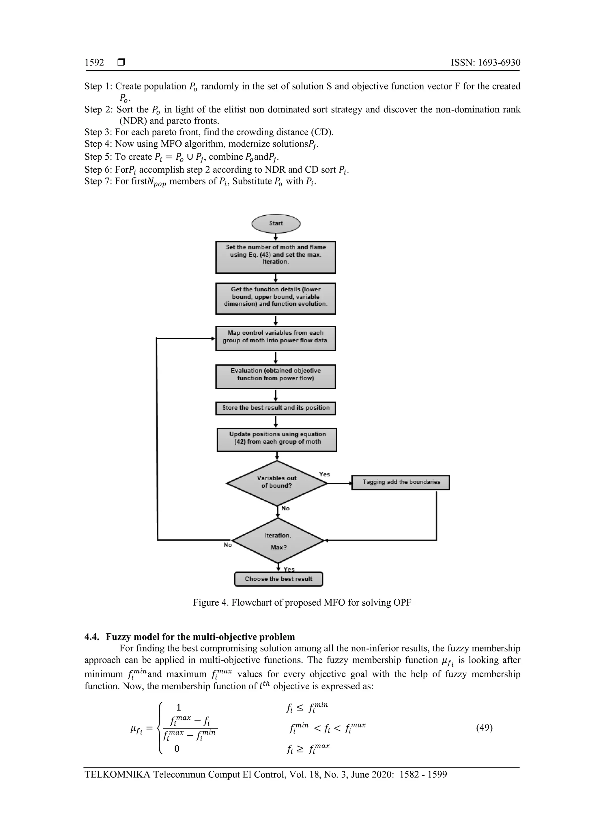
Flowchart of given MFO approach for resolving OPF issue is shown in Figure 4.
The method of the suggested non-sorting MFO approach has appeared in algorithm-1. Initially,
introduce parameters, for example, population size 𝑁𝑝𝑜𝑝, and stopping value, here it is the most extreme no. of
generation to proceeds the method. Besides, a random parent population 𝑃𝑜in possible space S is produced and
every objective function of the objective vector F for 𝑃𝑜 is assessed. Afterward, non-dominated sorting along
with crowding distance calculation as clarified in table [25] and is implemented on 𝑃𝑜. Subsequently, the MFO
approach is utilized to make the fresh population𝑃𝑗, and then it is converged with 𝑃𝑜 to shape the blended
population 𝑃𝑖. This 𝑃𝑖 is arranged in view of elitism non-domination, and in light of the figured estimations of
crowding distance (CD) and non-domination rank (NDR), the best 𝑁 𝑝𝑜𝑝 arrangements are refreshed to frame
another parent population. This procedure is repeated until the highest no. of generations (cycles) are come to.
It must be noticed that a similar approach can be utilized along with end criteria set according to the total
evaluations of the function.
Algorithm 1. Non-dominated moth flame optimization [25]

 ISSN: 1693-6930
1592
Step 1: Create population 𝑃𝑜 randomly in the set of solution S and objective function vector F for the created
𝑃𝑜.
Step 2: Sort the 𝑃𝑜 in light of the elitist non dominated sort strategy and discover the non-domination rank
(NDR) and pareto fronts.
Step 3: For each pareto front, find the crowding distance (CD).
Step 4: Now using MFO algorithm, modernize solutions𝑃𝑗.
Step 5: To create 𝑃𝑖 = 𝑃𝑜 ∪ 𝑃𝑗, combine 𝑃𝑜and𝑃𝑗.
Step 6: For𝑃𝑖 accomplish step 2 according to NDR and CD sort 𝑃𝑖.
Step 7: For first𝑁𝑝𝑜𝑝 members of 𝑃𝑖, Substitute 𝑃𝑜 with 𝑃𝑖.
Figure 4. Flowchart of proposed MFO for solving OPF
4.4. Fuzzy model for the multi-objective problem
For finding the best compromising solution among all the non-inferior results, the fuzzy membership
approach can be applied in multi-objective functions. The fuzzy membership function 𝜇 𝑓 𝑖
is looking after
minimum 𝑓𝑖
𝑚𝑖𝑛
and maximum 𝑓𝑖
𝑚𝑎𝑥
values for every objective goal with the help of fuzzy membership
function. Now, the membership function of 𝑖 𝑡ℎ
objective is expressed as:
𝜇 𝑓 𝑖
=
{
1 𝑓𝑖 ≤ 𝑓𝑖
𝑚𝑖𝑛
𝑓𝑖
𝑚𝑎𝑥
− 𝑓𝑖
𝑓𝑖
𝑚𝑎𝑥
− 𝑓𝑖
𝑚𝑖𝑛 𝑓𝑖
𝑚𝑖𝑛
< 𝑓𝑖 <
0 𝑓𝑖 ≥ 𝑓𝑖
𝑚𝑎𝑥
𝑓𝑖
𝑚𝑎𝑥
(49)

1593
The values of membership functions lie in the scale of (0-1) and shows that how much it satisfies the
function 𝑓𝑖. Afterward, the decision-making function 𝜇 𝑘
should be computed as:
𝜇 𝑘
=
∑ 𝜇 𝑓 𝑖
𝑘𝑁
𝑖=1
∑ ∑ 𝜇 𝑓 𝑖
𝑘𝑁
𝑖=1
𝑀
𝑘=1
(50)
the decision-making function can also be considered as the normalized membership function for non-inferior
results and shows the ranking of the non-dominated results. The final result is treated as the best compromising
solution among all the pareto front having the value 𝑚𝑎𝑥𝑖𝑚𝑢𝑚 {𝜇 𝑘
: 𝑘 = 1,2,3 … … . . 𝑀}.
5. SIMULATION RESULTS AND ANALYSIS
In this analysis, the single objective and multi-objective optimization using MFO algorithm are
implemented to solve the stochastic OPF problem with wind and solar power plants. The adapted IEEE-30 bus
framework with wind and solar PV plants can be utilized to show the adequacy of the suggested approach. The
line information, load information and the data of wind and solar power plants are directly taken from [23].
The primary qualities of adapted IEEE-30 bus framework are given in Table 1. There are basically two cases
each having two scenarios as given below;
Part-A optimal power flow with two winds and one solar power plants.
Here, total 10 dissimilar test cases are considered as presented in Table 4. Outcomes of the case studies
considering moth flame approach are tabularized and described in this section. The first six case studies are for
single objectives optimization and rest of the cases are multi-objective optimization problems incorporated
with solar and wind power plants. In proposed work, the programming is done with MATLAB programming
language and calculated on the system having 3.4 GHz Intel i5 processor with 8 GB RAM. Here, the search
agent value is choosing to be 40 and each algorithm is analyzed for 10 independent runs with 500 iterations
per run.
Table 4. Summary of case studies for adapted IEEE-30 bus test system
Test system Case # Single and multi-objectives functions
IEEE
30-bus test
system
(modified)
Case # 1 Minimization total fuel cost.
Case # 2 Emission minimization.
Case # 3 Voltage deviation minimization.
Case # 4 Active power loss minimization.
Case # 5 Voltage stability enhancement.
Case # 6 Total Fuel Cost with carbon Tax minimization.
Case # 7 Total Fuel Cost and Emission minimization.
Case # 8 Total Fuel Cost, Emission, and active power loss minimization.
Case # 9 Total Fuel Cost, Emission, and voltage deviation minimization.
Case # 10 Total Fuel Cost, Emission, Voltage deviation and active power loss minimization.
5.1. Scenario-1 (single objective OPF with wind and solar PV plants)
Here all the objective goals specified in mathematical formulation and are solved as solo objective
optimization issue with the help of a moth flame optimization approach. The limits of all control variables like,
voltage magnitudes of all the generators and transformer tap settings are lies in a span of [0.9-1.1] p.u.
The upper and lower voltage span of all PQ buses taken between [0.95-1.1] p.u, and the reactive power
compensator having the rating between 0 to 5 MVAr. The best minimum values of the objective functions
starting from case-1 to case-6 with control variables are tabulated in Table 5.
The overall fuel cost including the renewable solar and wind power plants cost in case-1 is
780.485 $/hr which is reduced up to 2.018 $/hr in comparison with [23] which is tabulated in Table 6.
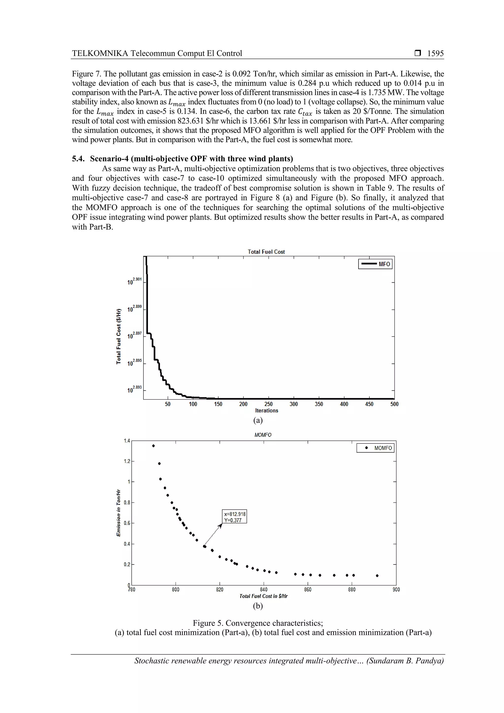
The convergence curve of case-1 is displayed in Figure 5 (a). The pollutant gas emission in case-2 is
0.092 Ton/hr. Similarly, the voltage deviation of each bus from the 1.0 per unit is also a significant aspect for
a reliable operation of the grid. So, in a case-3, the minimum voltage variation is 0.298 p.u. The active power
loss of different transmission lines in case-4 is 1.735 MW.
The voltage stability index, also known as 𝐿 𝑚𝑎𝑥 index fluctuates from 0 (no load) to 1
(voltage collapse). So, the minimum value for the 𝐿 𝑚𝑎𝑥 index in case-5 is 0.134. In case-6, the carbon tax rate
𝐶𝑡𝑎𝑥 is taken as 20 $/Tonne [23]. The simulation result of total cost with emission is 809.969 $/hr which is less
compared to reference [23] shown in Table 6. After comparing the simulation outcomes, it is seen that
the proposed method of moth flame optimization technique gives the better results as shown in Figure 5 (b).

 ISSN: 1693-6930
1594
Table 5. Single objectives simulation results obtained for the system under study (Part-A)
Control variables Max Min Case-1 Case-2 Case-3 Case-4 Case-5 Case-6
PG2(Thermal) 80.00 20.00 27.516 46.634 80.000 60.741 20.000 33.275
PG8(Thermal) 35.00 10.00 10.000 35.000 35.000 35.000 35.000 10.000
PG5(Wind) 75.00 0.00 43.868 75.000 75.000 75.000 65.311 45.974
PG11(Wind) 60.00 0.00 37.140 53.681 2.010 60.000 60.000 38.793
PG13(Solar) 50.00 0.00 35.431 44.183 0.000 46.439 25.271 36.715
VG1 1.10 0.95 1.100 0.950 0.950 1.100 0.950 1.100
VG2 1.10 0.95 1.089 0.974 0.950 1.100 1.100 1.090
VG5 1.10 0.95 1.070 1.036 0.999 1.091 1.100 1.071
VG8 1.10 0.95 1.100 1.100 1.094 1.100 1.100 1.100
VG11 1.10 0.95 1.100 1.100 1.100 1.100 1.100 1.100
VG13 1.10 0.95 1.094 1.100 1.056 1.100 1.100 1.095
QC10 5.00 0.00 4.985 5.000 5.000 1.426 5.000 5.000
QC12 5.00 0.00 5.000 0.000 0.000 5.000 4.030 5.000
QC15 5.00 0.00 0.000 5.000 4.850 4.933 5.000 0.000
QC17 5.00 0.00 0.000 3.723 0.052 0.000 5.000 4.757
QC20 5.00 0.00 5.000 5.000 5.000 5.000 5.000 0.000
QC21 5.00 0.00 0.013 5.000 5.000 0.046 4.959 5.000
QC23 5.00 0.00 0.004 5.000 1.019 5.000 5.000 5.000
QC24 5.00 0.00 0.083 2.057 5.000 0.006 0.000 0.000
QC29 5.00 0.00 5.000 5.000 5.000 4.990 5.000 5.000
T11(6-9) 1.10 0.9 0.900 1.086 1.100 1.100 0.900 0.900
T12(6-10) 1.10 0.9 0.922 0.916 1.100 0.900 1.019 0.900
T15(4-12) 1.10 0.9 1.099 0.900 0.900 0.916 1.100 1.100
T36(28-27) 1.10 0.9 1.100 1.100 1.100 1.066 1.100 1.100
Total F.C ($/h) - - 780.485 914.017 1013.712 957.229 919.634 _
Emission (T/h) - - 1.762 0.092 0.358 0.100 0.264 0.898
V.D (p.u) - - 1.046 0.410 0.298 1.342 1.379 1.067
Ploss(MW) - - 5.464 3.752 14.581 1.735 3.062 5.010
Lmax - - _ _ _ _ 0.134 _
Total F.C with a carbon
tax ($/h)
- - _ _ _ _ _ 809.969
Table 6. Comparison of the simulation results for single objectives (Part-A)
Single objectives functions Proposed MFO SHADE [23]
Total F.C ($/h) 780.485 782.503
Emission (T/h) 0.092 NA
V.D (p.u) 0.298 NA
Ploss (MW) 1.735 NA
Lmax 0.134 NA
Total F.C with a carbon tax ($/h) 809.969 810.346
5.2. Scenario-2 (Multi-objective OPF with wind and solar PV plants)
In this scenario, two objectives, three objectives and four objectives optimized simultaneously with
the moth flame optimization approach. In the multi-objective optimization, the non-dominated sorting optimization
technique is applied for finding the archives of different objectives simultaneously. Here, 30 non-dominates solutions
are maintained for finding the pareto front for IEEE 30-bus framework. The case-7 to case-10 are treated as
the multi-objective optimization problems for IEEE 30-bus framework with wind and solar plants. For finding
the best compromising solution among all the pareto archives, the fuzzy decision-making approach is employed.
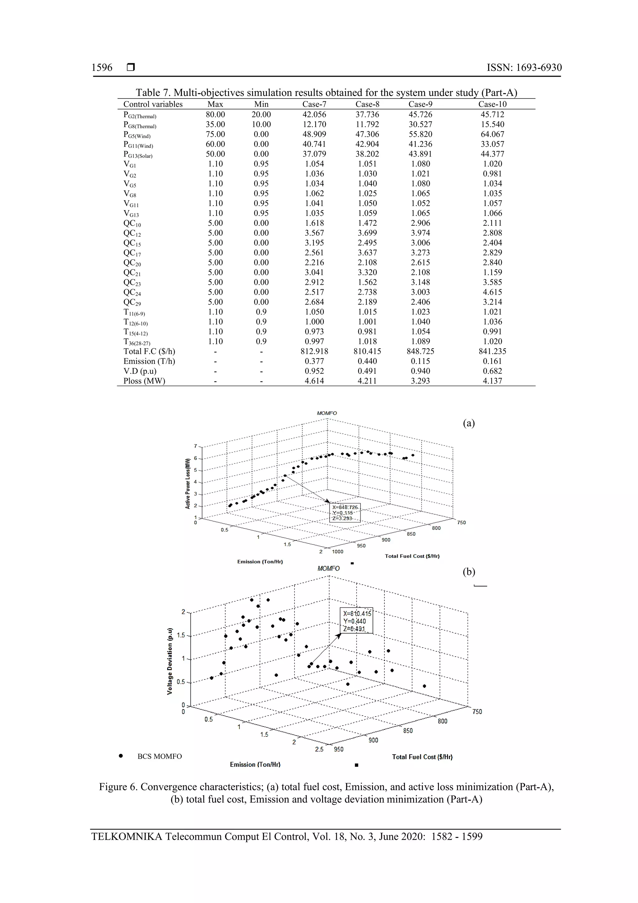
The finest compromising solutions for the different cases are demonstrated in boldfaced and mentioned in Table 7.
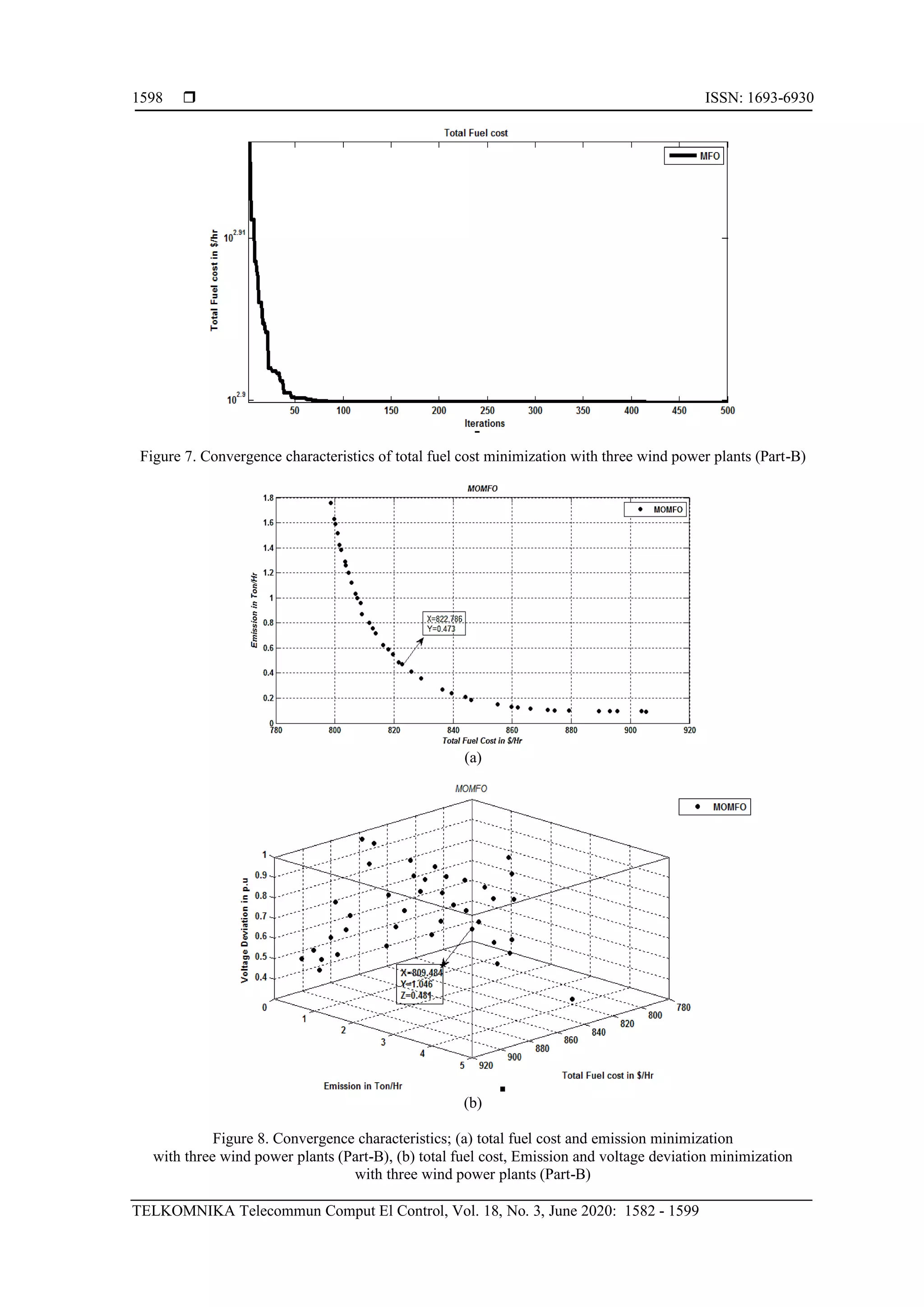
The finest compromise solutions are obtained using the moth flame optimization techniques with the case-7 is
displayed in Figure 5 (b). The pareto front of case-8 and case-9 are displayed in Figure 6 (a) and Figure 6 (b).
It is come to know that the MOMFO approach is one of the best approaches for searching the optimal solutions of
the multi-objective OPF issue integrating solar and wind plants. Part-B optimal power flow with three winds
power plants. Here, the solar power plant at bus number-13 is replaced with another wind farm to check
the techno-economic impact on optimal power flow issue. The parameters of are given into the Table 3. There are
also the similar cases of single and multi-objective optimization are taken. The control variables and maximum and
minimum limits are same as Part-A.
5.3. Scenario-3 (single objective OPF with three wind power plants)
Here the all objectives are treated as the single objectives and optimized with the help of moth flame
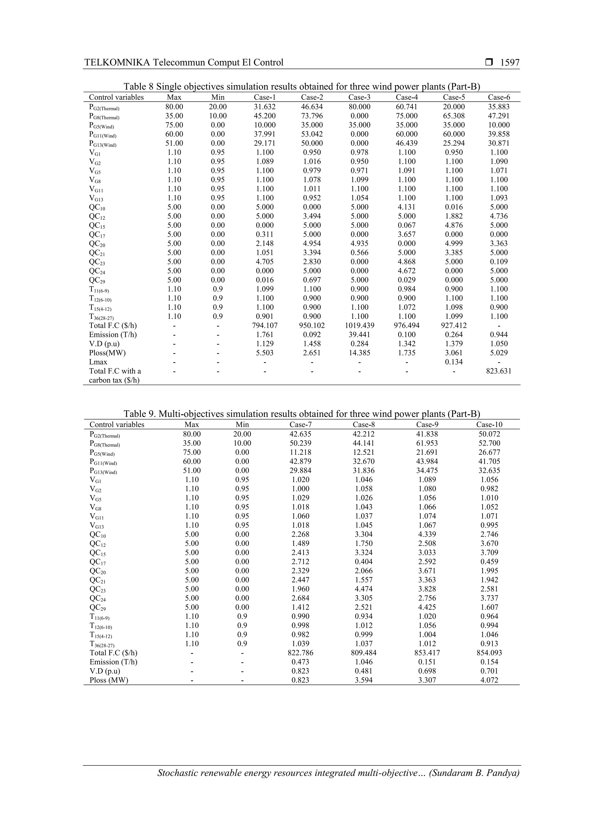
optimization algorithm. The best optimized results are tabulated in Table 8. For Case-1, the total fuel cost including
three renewable wind power plants as in case-1 is 794.107 $/hr which is increased up to 13.622 $/hr in comparison
with fuel cost of part-A which is tabulated in Table 6. The convergence curve of total fuel cost is displayed in

1595
Figure 7. The pollutant gas emission in case-2 is 0.092 Ton/hr, which similar as emission in Part-A. Likewise, the
voltage deviation of each bus that is case-3, the minimum value is 0.284 p.u which reduced up to 0.014 p.u in
comparison with the Part-A. The active power loss ofdifferent transmission lines in case-4 is 1.735 MW. The voltage
stability index, also known as 𝐿 𝑚𝑎𝑥 index fluctuates from 0 (no load) to 1 (voltage collapse). So, the minimum value
for the 𝐿 𝑚𝑎𝑥 index in case-5 is 0.134. In case-6, the carbon tax rate 𝐶𝑡𝑎𝑥 is taken as 20 $/Tonne. The simulation
result of total cost with emission 823.631 $/hr which is 13.661 $/hr less in comparison with Part-A. After comparing
the simulation outcomes, it shows that the proposed MFO algorithm is well applied for the OPF Problem with the
wind power plants. But in comparison with the Part-A, the fuel cost is somewhat more.
5.4. Scenario-4 (multi-objective OPF with three wind plants)
As same way as Part-A, multi-objective optimization problems that is two objectives, three objectives
and four objectives with case-7 to case-10 optimized simultaneously with the proposed MFO approach.
With fuzzy decision technique, the tradeoff of best compromise solution is shown in Table 9. The results of
multi-objective case-7 and case-8 are portrayed in Figure 8 (a) and Figure (b). So finally, it analyzed that
the MOMFO approach is one of the techniques for searching the optimal solutions of the multi-objective
OPF issue integrating wind power plants. But optimized results show the better results in Part-A, as compared
with Part-B.
(a)
(b)
Figure 5. Convergence characteristics;
(a) total fuel cost minimization (Part-a), (b) total fuel cost and emission minimization (Part-a)

 ISSN: 1693-6930
1596
Table 7. Multi-objectives simulation results obtained for the system under study (Part-A)
Control variables Max Min Case-7 Case-8 Case-9 Case-10
PG2(Thermal) 80.00 20.00 42.056 37.736 45.726 45.712
PG8(Thermal) 35.00 10.00 12.170 11.792 30.527 15.540
PG5(Wind) 75.00 0.00 48.909 47.306 55.820 64.067
PG11(Wind) 60.00 0.00 40.741 42.904 41.236 33.057
PG13(Solar) 50.00 0.00 37.079 38.202 43.891 44.377
VG1 1.10 0.95 1.054 1.051 1.080 1.020
VG2 1.10 0.95 1.036 1.030 1.021 0.981
VG5 1.10 0.95 1.034 1.040 1.080 1.034
VG8 1.10 0.95 1.062 1.025 1.065 1.035
VG11 1.10 0.95 1.041 1.050 1.052 1.057
VG13 1.10 0.95 1.035 1.059 1.065 1.066
QC10 5.00 0.00 1.618 1.472 2.906 2.111
QC12 5.00 0.00 3.567 3.699 3.974 2.808
QC15 5.00 0.00 3.195 2.495 3.006 2.404
QC17 5.00 0.00 2.561 3.637 3.273 2.829
QC20 5.00 0.00 2.216 2.108 2.615 2.840
QC21 5.00 0.00 3.041 3.320 2.108 1.159
QC23 5.00 0.00 2.912 1.562 3.148 3.585
QC24 5.00 0.00 2.517 2.738 3.003 4.615
QC29 5.00 0.00 2.684 2.189 2.406 3.214
T11(6-9) 1.10 0.9 1.050 1.015 1.023 1.021
T12(6-10) 1.10 0.9 1.000 1.001 1.040 1.036
T15(4-12) 1.10 0.9 0.973 0.981 1.054 0.991
T36(28-27) 1.10 0.9 0.997 1.018 1.089 1.020
Total F.C ($/h) - - 812.918 810.415 848.725 841.235
Emission (T/h) - - 0.377 0.440 0.115 0.161
V.D (p.u) - - 0.952 0.491 0.940 0.682
Ploss (MW) - - 4.614 4.211 3.293 4.137
Figure 6. Convergence characteristics; (a) total fuel cost, Emission, and active loss minimization (Part-A),
(b) total fuel cost, Emission and voltage deviation minimization (Part-A)
(a)
(b)
• BCS MOMFO

1597
Table 8 Single objectives simulation results obtained for three wind power plants (Part-B)
Control variables Max Min Case-1 Case-2 Case-3 Case-4 Case-5 Case-6
PG2(Thermal) 80.00 20.00 31.632 46.634 80.000 60.741 20.000 35.883
PG8(Thermal) 35.00 10.00 45.200 73.796 0.000 75.000 65.308 47.291
PG5(Wind) 75.00 0.00 10.000 35.000 35.000 35.000 35.000 10.000
PG11(Wind) 60.00 0.00 37.991 53.042 0.000 60.000 60.000 39.858
PG13(Wind) 51.00 0.00 29.171 50.000 0.000 46.439 25.294 30.871
VG1 1.10 0.95 1.100 0.950 0.978 1.100 0.950 1.100
VG2 1.10 0.95 1.089 1.016 0.950 1.100 1.100 1.090
VG5 1.10 0.95 1.100 0.979 0.971 1.091 1.100 1.071
VG8 1.10 0.95 1.100 1.078 1.099 1.100 1.100 1.100
VG11 1.10 0.95 1.100 1.011 1.100 1.100 1.100 1.100
VG13 1.10 0.95 1.100 0.952 1.054 1.100 1.100 1.093
QC10 5.00 0.00 5.000 0.000 5.000 4.131 0.016 5.000
QC12 5.00 0.00 5.000 3.494 5.000 5.000 1.882 4.736
QC15 5.00 0.00 0.000 5.000 5.000 0.067 4.876 5.000
QC17 5.00 0.00 0.311 5.000 0.000 3.657 0.000 0.000
QC20 5.00 0.00 2.148 4.954 4.935 0.000 4.999 3.363
QC21 5.00 0.00 1.051 3.394 0.566 5.000 3.385 5.000
QC23 5.00 0.00 4.705 2.830 0.000 4.868 5.000 0.109
QC24 5.00 0.00 0.000 5.000 0.000 4.672 0.000 5.000
QC29 5.00 0.00 0.016 0.697 5.000 0.029 0.000 5.000
T11(6-9) 1.10 0.9 1.099 1.100 0.900 0.984 0.900 1.100
T12(6-10) 1.10 0.9 1.100 0.900 0.900 0.900 1.100 1.100
T15(4-12) 1.10 0.9 1.100 0.900 1.100 1.072 1.098 0.900
T36(28-27) 1.10 0.9 0.901 0.900 1.100 1.100 1.099 1.100
Total F.C ($/h) - - 794.107 950.102 1019.439 976.494 927.412 -
Emission (T/h) - - 1.761 0.092 39.441 0.100 0.264 0.944
V.D (p.u) - - 1.129 1.458 0.284 1.342 1.379 1.050
Ploss(MW) - - 5.503 2.651 14.385 1.735 3.061 5.029
Lmax - - - - - - 0.134 -
Total F.C with a
carbon tax ($/h)
- - - - - - - 823.631
Table 9. Multi-objectives simulation results obtained for three wind power plants (Part-B)
Control variables Max Min Case-7 Case-8 Case-9 Case-10
PG2(Thermal) 80.00 20.00 42.635 42.212 41.838 50.072
PG8(Thermal) 35.00 10.00 50.239 44.141 61.953 52.700
PG5(Wind) 75.00 0.00 11.218 12.521 21.691 26.677
PG11(Wind) 60.00 0.00 42.879 32.670 43.984 41.705
PG13(Wind) 51.00 0.00 29.884 31.836 34.475 32.635
VG1 1.10 0.95 1.020 1.046 1.089 1.056
VG2 1.10 0.95 1.000 1.058 1.080 0.982
VG5 1.10 0.95 1.029 1.026 1.056 1.010
VG8 1.10 0.95 1.018 1.043 1.066 1.052
VG11 1.10 0.95 1.060 1.037 1.074 1.071
VG13 1.10 0.95 1.018 1.045 1.067 0.995
QC10 5.00 0.00 2.268 3.304 4.339 2.746
QC12 5.00 0.00 1.489 1.750 2.508 3.670
QC15 5.00 0.00 2.413 3.324 3.033 3.709
QC17 5.00 0.00 2.712 0.404 2.592 0.459
QC20 5.00 0.00 2.329 2.066 3.671 1.995
QC21 5.00 0.00 2.447 1.557 3.363 1.942
QC23 5.00 0.00 1.960 4.474 3.828 2.581
QC24 5.00 0.00 2.684 3.305 2.756 3.737
QC29 5.00 0.00 1.412 2.521 4.425 1.607
T11(6-9) 1.10 0.9 0.990 0.934 1.020 0.964
T12(6-10) 1.10 0.9 0.998 1.012 1.056 0.994
T15(4-12) 1.10 0.9 0.982 0.999 1.004 1.046
T36(28-27) 1.10 0.9 1.039 1.037 1.012 0.913
Total F.C ($/h) - - 822.786 809.484 853.417 854.093
Emission (T/h) - - 0.473 1.046 0.151 0.154
V.D (p.u) - - 0.823 0.481 0.698 0.701
Ploss (MW) - - 0.823 3.594 3.307 4.072

 ISSN: 1693-6930
1598
Figure 7. Convergence characteristics of total fuel cost minimization with three wind power plants (Part-B)
(a)
(b)
Figure 8. Convergence characteristics; (a) total fuel cost and emission minimization
with three wind power plants (Part-B), (b) total fuel cost, Emission and voltage deviation minimization
with three wind power plants (Part-B)

1599
6. CONCLUSION
This paper proposed the solution technique to single and multi-objective optimal power flow (MOOPF)
issue containing thermal power plants plus solar and wind power plants. The paper contains the techno-economic
analysis of two parts. The first part contains the two wind and one solar power plants and the analysis of the OPF
problem. The performances are compared with recently available optimization technique. From the obtained result,
the suggested MOMFO accomplishes improved quality and additionally feasible solutions for each situation of
optimal power flow and has better convergence compare to other algorithms. In second part, the solar PV plant is
replaced with the wind power plant and the solution of optimal power flow issue. The results are compared with the
two different parts. From the techno-economic analysis, the multi-objective OPF problem with the two wind power
plants and one solar power plant having less total fuel cost in comparison with the three wind power plants. So
finally, it is shown that with a non-dominated sorting method, MOMFO can be proficiently utilized for solving small
and large optimal power flow issues by incorporating wind and solar power plants.
REFERENCES
[1] J. L. Carpentier, “Optimal power flows uses, methods, and developments,” IFAC Proc. Vol., vol. 18, no. 7, pp. 11-21, 1985.
[2] K. S. Pandya and S. K. Joshi, “A survey of Optimal Power Flow methods,” Journal Appl. Inf. Technolology, vol. 4,
no. 5, pp. 450-458, 2005.
[3] D. H. Wolpert and W. G. Macready, “No free lunch theorems for optimization,” IEEE Trans. Evol. Comput., vol. 1,
no. 1, pp. 67-82, 1997.
[4] M. M. A. M. Abido, “Optimal power flow using particle swarm optimization,” J. Electr. Power Energy Syst., vol. 24,
no. 7, pp. 563-571, 2002.
[5] M. A. Abido, “Optimal power flow using tabu search algorithm,” Electr. Power Components System, vol. 30, no. 5,
pp. 469-483, 2002.
[6] L. L. Lai, J. T. Ma, R. Yokoyama, and M. Zhao, “Improved genetic algorithms for optimal power flow under both
normal and contingent operation states,” Int. J. Electr. Power Energy Syst., vol. 19, no. 5, pp. 287-292, 1997.
[7] H. R. E. H. Bouchekara, A. E. Chaib, M. A. Abido, and R. A. El-Sehiemy, “Optimal power flow using an improved
colliding bodies optimization algorithm,” Appl. Soft Comput., vol. 42, pp. 119-131, 2016.
[8] H. R. E. H. Bouchekara, “Optimal power flow using black-hole-based optimization approach,” Appl. Soft Computing,
vol. 24, pp. 879-888, 2014.
[9] A. A. A. Mohamed, Y. S. Mohamed, A. A. M. El-Gaafary, and A. M. Hemeida, “Optimal power flow using moth
swarm algorithm,” Electr. Power Syst. Res., vol. 142, pp. 190-206, 2017.
[10] S. S. Reddy and C. S. Rathnam, “Optimal power flow using glowworm swarm optimization,” Int. J. Electr. Power
Energy Syst., vol. 80, pp. 128-139, 2016.
[11] A. E. A. Chaib, H. R. E. H. Bouchekara, R. Mehasni, and M. A. Abido, “Optimal power flow with emission and non-
smooth cost functions using backtracking search optimization algorithm,” Int. J. Electr. Power Energy Syst., vol. 81,
pp. 64-77, 2016.
[12] H. R. E. H. Bouchekara, A. E. Chaib, M. A. Abido, and R. A. El-Sehiemy, “Optimal power flow using an Improved
Colliding Bodies Optimization algorithm,” Appl. Soft Comput., vol. 42, pp. 119-131, 2016.
[13] R. Roy and H. T. Jadhav, “Optimal power flow solution of power system incorporating stochastic wind power using
Gbest guided artificial bee colony algorithm,” Int J Electr Power Energy Syst, vol. 64, pp. 562-78, 2015.
[14] A. Panda and M. Tripathy, “Optimal power flow solution of wind integrated power system using modified bacteria
foraging algorithm,” Int. J. Electr. Power Energy Syst., vol. 54, pp. 306-314, 2014.
[15] A. Panda and M. Tripathy, “Security constrained optimal power flow solution of wind-thermal generation system
using modified bacteria foraging algorithm,” Energy, vol. 93, part 1, pp. 816-827, 2015.
[16] L. Shi, C. Wang, L. Yao, Y. Ni, and M. Bazargan, “Optimal power flow solution incorporating wind power,” IEEE
Syst. J., vol. 6, no. 2, pp. 233-241, 2012.
[17] R. A. Jabr and B. C. Pal, “Intermittent wind generation in optimal power flow dispatching,” IET Gener. Transm.
Distrib., vol. 3, no. 1, pp. 66-74, 2009.
[18] S. Mishra, Y. Mishra, and S. Vignesh. “Security constrained economic dispatch considering wind energy conversion
systems,” Power and Energy Society General Meeting, pp. 1-8, 2011.
[19] Z. Wei, P. Yu, and S. Hui. “Optimal wind-thermal coordination dispatch based on risk reserve constraints.” Europ.
Transact. Elect. Power, vol. 21, no. 1, pp. 740-756, 2011.
[20] H. M. Dubey, M. Pandit, and B. K. Panigrahi, “Hybrid flower pollination algorithm with time-varying fuzzy selection
mechanism for wind integrated multi-objective dynamic economic dispatch,” Renewable Energy vol. 83, pp.188-202, 2015.
[21] H. Tazvinga, B. Zhu, and X. Xia “Optimal power flow management for distributed energy resources with batteries,”
Energy Convers Manage, vol. 102, pp. 104-110, 2015.
[22] K. Kusakana, “Optimal scheduling for distributed hybrid system with pumped hydro storage.” Energy Convers.
Manage., vol. 111, pp. 253-260, 2016.
[23] P. P. Biswas, P. N. Suganthan, and G. A. J. Amartunga, “Optimal power flow solutions incorporating stochastic wind
and solar,” Energy Conversion and Managemant, vol. 148, pp. 1194-1207, 2017.
[24] S. Mirjalili, “Moth-flame optimization algorithm: A novel nature-inspired heuristic paradigm,” Knowledge-Based
Syst., vol. 89, pp. 228-249, 2015.
[25] V. Savsani and M. A. Tawhid, “Non-dominated sorting moth flame optimization (NS-MFO) for multi-objective
problems,” Engineering Applications for Artificial Intelligence., vol. 63, pp. 20-32, 2017.

Stochastic renewable energy resources integrated multi-objective optimal power flow

More Related Content

What's hot

Similar to Stochastic renewable energy resources integrated multi-objective optimal power flow

More from TELKOMNIKA JOURNAL

Recently uploaded

Stochastic renewable energy resources integrated multi-objective optimal power flow