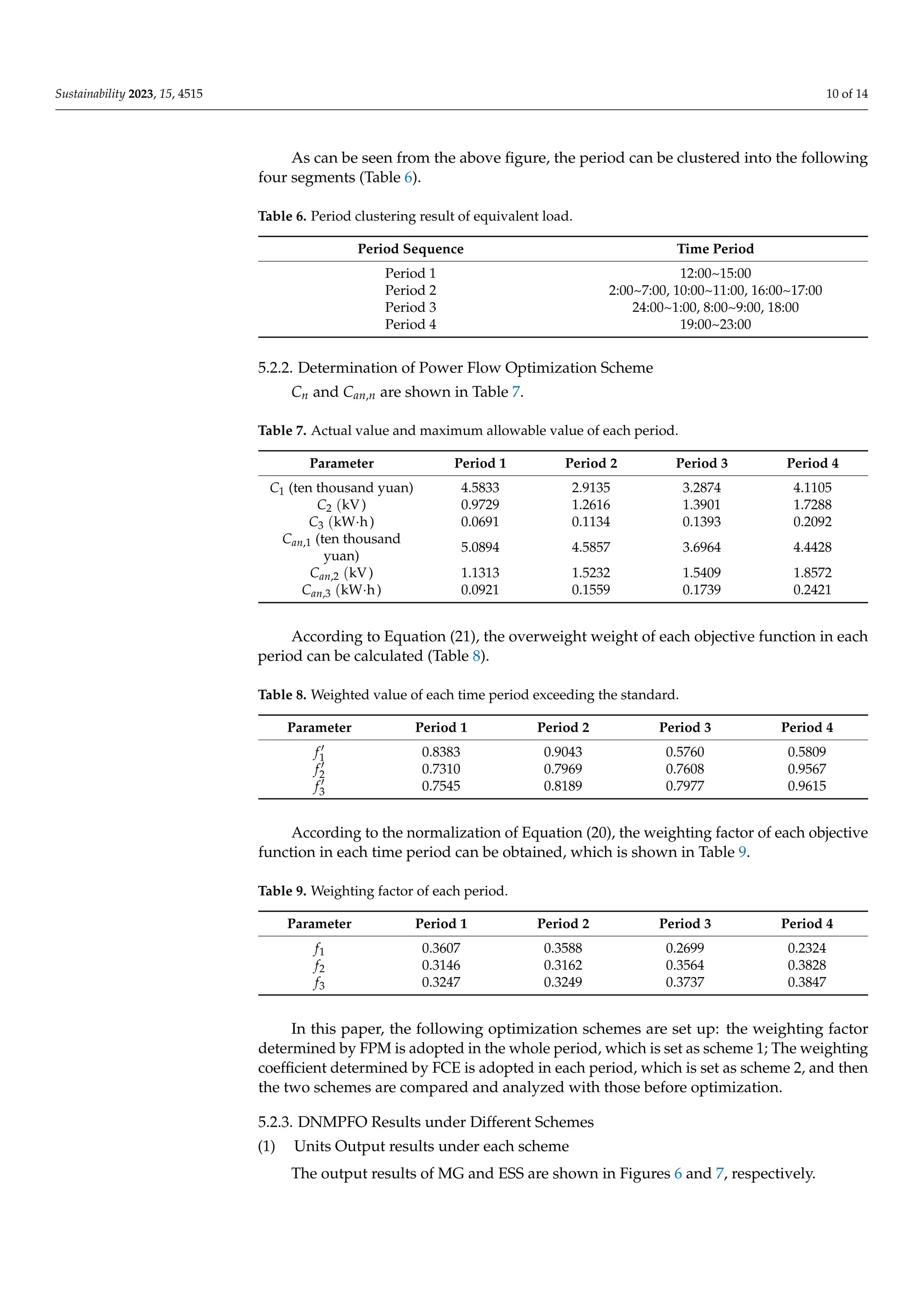
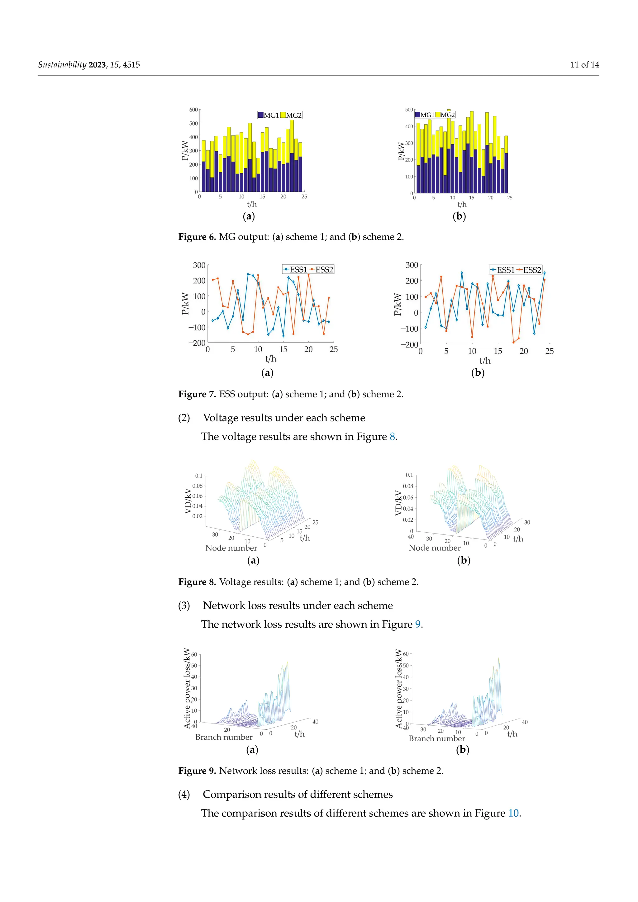
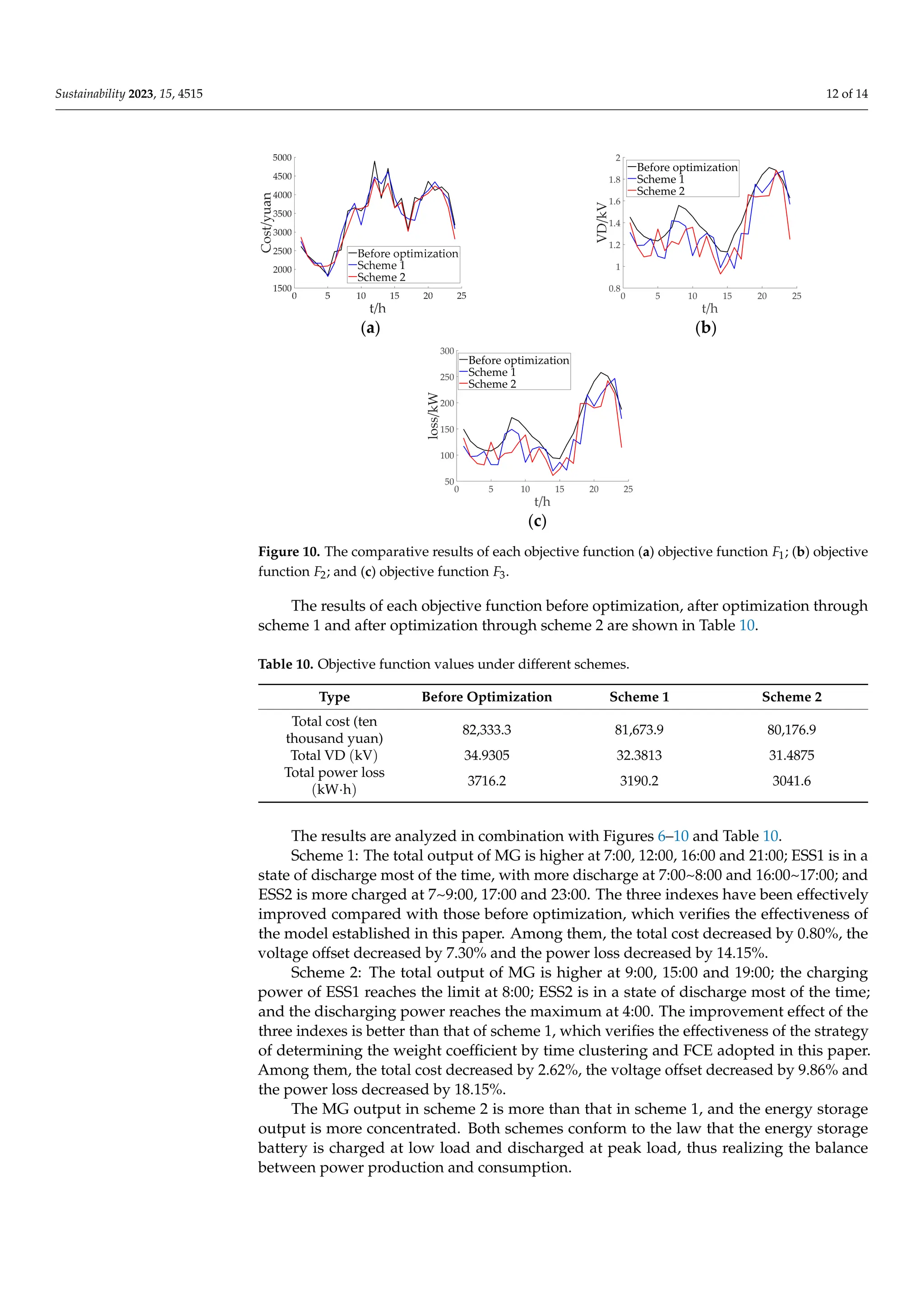
This document presents a power flow optimization strategy model for a distribution network that considers source, load, and storage. The model aims to minimize total cost, voltage deviation, and power losses over time periods determined through k-means clustering of an equivalent load curve. A particle swarm optimization algorithm is used to solve the multi-objective optimization model subject to power flow, voltage, and other constraints. The model is tested on an IEEE 33-node system and is shown to improve economic and reliability performance compared to a fixed weighting approach.
![Citation: Zheng, F.; Meng, X.; Wang,
L.; Zhang, N. Power Flow
Optimization Strategy of Distribution
Network with Source and Load
Storage Considering Period
Clustering. Sustainability 2023, 15,
4515. https://doi.org/
10.3390/su15054515
Academic Editors: Fu Gu,
Jingxiang Lv and Shun Jia
Received: 1 February 2023
Revised: 25 February 2023
Accepted: 1 March 2023
Published: 2 March 2023
Copyright: © 2023 by the authors.
Licensee MDPI, Basel, Switzerland.
This article is an open access article
distributed under the terms and
conditions of the Creative Commons
Attribution (CC BY) license (https://
creativecommons.org/licenses/by/
4.0/).
sustainability
Article
Power Flow Optimization Strategy of Distribution Network
with Source and Load Storage Considering Period Clustering
Fangfang Zheng , Xiaofang Meng *, Lidi Wang and Nannan Zhang
College of Information and Electric Engineering, Shenyang Agricultural University, Shenyang 110866, China
* Correspondence: xfmeng123@syau.edu.cn; Tel.: +86-158-0244-6563
Abstract: The large-scale grid connection of new energy will affect the optimization of power flow.
In order to solve this problem, this paper proposes a power flow optimization strategy model of a
distribution network with non-fixed weighting factors of source, load and storage. The objective
function is the lowest cost, the smallest voltage deviation and the smallest power loss, and many
constraints, such as power flow constraint, climbing constraint and energy storage operation con-
straint, are also considered. Firstly, the equivalent load curve is obtained by superimposing the
output of wind and solar turbines with the initial load, and the best k value is obtained by the elbow
rule. The k-means algorithm is used to cluster the equivalent load curve in different periods, and
then the fuzzy comprehensive evaluation method is used to determine the weighting factor of the
optimization model in each period. Then, the particle swarm optimization algorithm is used to solve
the multi-objective power flow optimization model, and the optimal strategy and objective function
values of each unit output in the operation period are obtained. Finally, IEEE33 is used as an example
to verify the effectiveness of the proposed model through two cases: a fixed proportion method to
determine the weighting factor, and this method to determine the weighting factor. The proposed
method can improve the economy and reliability of distribution networks.
Keywords: distribution network; power flow optimization; k-means period clustering; energy storage
system; particle swarm optimization
1. Introduction
As the power grid continues to develop in a more efficient, flexible and sustainable
direction [1,2], the large-scale grid connection of distributed new energy has become an
inevitable trend [3,4], increasing the difficulty of multi-objective power flow optimization
(DNMPFO) of distribution networks [5–7].
At present, scholars at home and abroad have carried out relevant research on DN-
MPFO. Reference [8] generated a typical wind-light-load scenario based on fuzzy C-means
clustering algorithm, and established a new energy planning model with the goal of max-
imizing the total installed capacity of distribution networks connected to scenery, but
energy storage was not involved in the model. Reference [9] clustered wind speed and
irradiance, and proposed a two-level optimal allocation model. The upper model took
the comprehensive income as the goal, and the lower model took the minimum sum of
network loss and voltage deviation as the goal, and adopted the planning-optimization
solution strategy of genetic algorithm-interior point method, but energy storage is not
considered in this reference either. Reference [10] established a mathematical model of
interval power flow optimization (PFO) of an AC/DC hybrid system with a DC power
flow controller based on interval and affine arithmetic, and used a non-dominated se-
quencing genetic algorithm to solve the model. However, the cost of unit operation is not
considered in the model. Reference [11] modeled the uncertainty of wind and solar power
generation, established a multi-objective optimization model of a battery energy storage
system coordinated with demand response, and used a non-sequential genetic algorithm
Sustainability 2023, 15, 4515. https://doi.org/10.3390/su15054515 https://www.mdpi.com/journal/sustainability](https://image.slidesharecdn.com/sustainability-15-04515-v31-240415040702-25ace7d3/75/stability-of-power-flow-analysis-of-different-resources-both-on-and-off-grid-1-2048.jpg)
![Sustainability 2023, 15, 4515 2 of 14
to solve it. However, photovoltaic units are not involved in this reference. Reference [12]
proposed a multi-objective optimization hierarchical strategy of a distribution network
considering the integration of distributed power generation and electric vehicles, which
was solved by a genetic algorithm, but the wind turbine unit was not considered in the
model. Considering the correlation, reference [13] simulated a 33-node distribution net-
work, and the results showed that although the cost and network loss decrease, the voltage
deviation increased slightly. Among the existing references on power flow optimization of
distribution networks, there are very few references considering new energy and energy
storage such as wind and solar, and none of them involve time period clustering, which
needs further study.
For the DNMPFO problem with source load storage (SLS), this paper proposes a
time-phased PFO model of a distribution network that takes into account many constraints,
and uses a particle swarm optimization algorithm to solve the model. Finally, the paper
takes a IEEE33-bus system as an example to carry out simulation analysis on the Matlab
software (Version is R2016a) to verify the effectiveness of the proposed model in solving
power flow optimization problems. The main contributions of this work are summarized
as follows:
(1) Based on the k-means clustering method, the equivalent load curve is clustered in
different periods, so as to dynamically determine the weight coefficient of the objective
function according to the periods;
(2) A solution method based on particle swarm optimization is proposed, which can
effectively solve the model.
(3) Based on the proposed power flow optimization method of distribution network
considering time period clustering, the power flow optimization of the IEEE33 system
in a certain area is analyzed, and the objective function values are all decreased, thus
improving the economy and security of the distribution network.
2. Multi-Objective Power Flow Optimization Model of Distribution Network with
Source and Load Storage
The DNMPFO model includes wind turbine (WT), photovoltaic unit (PV), micro gas
turbine (MG) and energy storage system (ESS). In order to make the optimization effect
of power flow better, in addition to the total economic cost, voltage offset and power
loss should also be considered. Since the model includes WT and PV with uncertain
characteristics, it may affect the stability of the power grid, and PFO is an important link to
ensure the stability, safety and economic operation of the power grid.
2.1. Establishment of Objective Function
(1) Objective function F1: the lowest total cost [14,15].
F1 = min
Cf + Cm + Cp,pur + Ch
(1)
where Cf is the unit fuel cost. Since PV and WT are clean energy, the fuel cost is zero.
The fuel cost of MG is calculated according to Equation (2), ten thousand yuan; Cm is the
operation and maintenance cost, calculated according to Equation (3), ten thousand yuan.
Because the structure of MG is convenient for monitoring and replacement repair, its opera-
tion and maintenance cost is not considered; Cp,pur is the cost of purchasing electricity from
the superior power grid, calculated according to Equation (4), ten thousand yuan; Ch is the
pollutant emission control cost, calculated according to Equation (5), ten thousand yuan.
Cf = 104
·
T
∑
t=1
NMG
∑
i=1
cgPunit,i
sgηMG
(2)](https://image.slidesharecdn.com/sustainability-15-04515-v31-240415040702-25ace7d3/75/stability-of-power-flow-analysis-of-different-resources-both-on-and-off-grid-2-2048.jpg)
![Sustainability 2023, 15, 4515 3 of 14
where cg is the natural gas price, yuan/m3; sg is the calorific value of natural gas, kW·h/m3;
NMG is the number of MG; Punit,i is the output power of the ith unit, kW; and ηMG is the
conversion efficiency of MG.
Cm = 104
·
T
∑
t=1
J
∑
i=1
comPunit,i(t) (3)
where J is the number of units; and com is the operation and maintenance cost of the unit
power, yuan/kW.
Cp,pur = 104
·
T
∑
t=1
p(t)Ppur(t) (4)
where p(t) is the electricity price at time t, yuan/kW; and Ppur(t) is the power purchased
at time t, kW.
Ch = 104
·
T
∑
t=1
NMG
∑
i=1
c1,CO2
ccetPunit,i(t)
ηMG
!
+ 104
·
T
∑
t=1
c2,CO2
ccet(1 + ε)Ppur(t)
!
(5)
where c1,CO2
and c2,CO2
are, respectively, the CO2 emission coefficients of natural gas and
coal-fired power plant combustion, kg/kW·h; ccet is the equivalent carbon tax, yuan/kg;
and is the line loss rate of the power grid, %.
(2) Objective function F2: the node voltage deviation is the smallest; that is, the voltage
distribution is the most reasonable [16].
F2 = min
T
∑
t=1
n
∑
i=1
Ui,t − UN
UN
(6)
where n is the number of independent nodes of the distribution network; t is the period
mark; T is the number of whole day periods; Ui,t is the voltage amplitude of the ith node
during t period, kV; and UN is the rated voltage of the ith node, kV.
(3) Objective function F3: minimum power loss.
F3 = min
T
∑
t=1
b
∑
k=1
Pk(t) − P0
k(t)
∆t (7)
where b is the number of branches; Pk(t) and P0
k(t) are, respectively, the head power and
end power of branch k, kW; and ∆t is a run time period, h.
2.2. Constraints
The optimization strategy needs to satisfy equality constraints such as power flow
constraint and power balance constraint, and inequality constraints such as bus voltage
constraint and climbing constraint.
2.2.1. Power Flow Constraint
For the operation of a distribution network, it is necessary to meet certain power flow
constraints [17]:
Pin,i(t) = ei,t
n
∑
j=1
(Gijej,t − Bij fj,t) + fi,t
n
∑
j=1
(Gij fj,t + Bijej,t)
Qin,i(t) = fi,t
n
∑
j=1
(Gijej,t − Bij fj,t) − ei,t
n
∑
j=1
(Gij fj,t + Bijej,t)
(8)
where Pin,i and Qin,i are, respectively, the active power (kW) and reactive power (kVar)
injected into the distribution network by node i; ei,t and ji,t are, respectively, the real part
and imaginary part of the voltage of node i at time t; ej,t and jj,t are, respectively, the real](https://image.slidesharecdn.com/sustainability-15-04515-v31-240415040702-25ace7d3/75/stability-of-power-flow-analysis-of-different-resources-both-on-and-off-grid-3-2048.jpg)
![Sustainability 2023, 15, 4515 4 of 14
part and imaginary part of the voltage of node j at time t; Gij and Bij are, respectively, the
real part and imaginary part of elements in node admittance matrix, Ω.
2.2.2. Power Balance Constraints
The sum of the output of all units minus the load power and power loss is equal to the
power injected into the grid [18], with the following constraints:
(
Pin,i(t) = Pg,i(t) + PWT,i(t) + PPV,i(t) + Pdch
ESS,i(t) − Pch
ESS,i(t) + PMG,i(t) − PLoad,i(t) − PLoss
Qin,i(t) = Qg,i(t) + QMG,i(t) − QLoad,i(t) − QLoss
(9)
where Pg,i and Qg,i are, respectively, the active power (kW) and reactive power (kVar)
of the power supply on node i; PMG,i and QMG,i are, respectively, the active power (kW)
and reactive power (kVar) generated by the gas turbine on node i; Pdch
ESS,i and Pch
ESS,i are,
respectively, the discharge and charging power of the energy storage device on node i;
PLoad,i and QLoad,i are, respectively, the active load (kW) and reactive load (kVar) of node
i; and PLoss and QLoss are, respectively, the active power loss (kW) and reactive power
loss (kVar).
2.2.3. Bus Voltage Constraint
The bus voltage needs to meet the following constraints:
Ui,min ≤ Ui(t) ≤ Ui,max (10)
where Ui,max and Ui,min, respectively, represent the maximum and minimum value of the
voltage amplitude of the ith node, kV.
2.2.4. Unit Output Constraint
The unit output needs to meet the following constraints:
Pi,min ≤ Pi(t) ≤ Pi,max (11)
where Pi,max and Pi,min, respectively, represent the maximum and minimum value of the
active output of the ith unit, kW.
2.2.5. Energy Storage Operation Constraints
The output of the energy storage device during operation meets the following con-
straints [19]:
Pmin
ESS ≤ PESS(t) ≤ Pmax
ESS (12)
where PESS(t), Pmax
ESS and Pmin
ESS , respectively, represent the output power, the maximum
value of the output power and the minimum value of the output power of ESS at time
t, kW.
In order to prevent overcharging and discharging from affecting the battery life, the
overall state of charge (SOC) of ESS is constrained:
SOC(t) = (1 − γ)SOC0 +
T
∑
t=1
PESS(t)∆t
SOCmin ≤ SOC(t) ≤ SOCmax
(13)
where SOC(t) is the SOC value of ESS at time t, kW·h; γ is the self-discharge rate of
electric energy storage; and SOC0, SOCmin and SOCmax are, respectively, the initial value,
minimum value and maximum value of SOC, kW·h.](https://image.slidesharecdn.com/sustainability-15-04515-v31-240415040702-25ace7d3/75/stability-of-power-flow-analysis-of-different-resources-both-on-and-off-grid-4-2048.jpg)
![Sustainability 2023, 15, 4515 5 of 14
2.2.6. Climbing Constraint
According to the operation characteristics of MG, its active power regulation rate
(namely climbing rate) is constrained [20]:
Rdown ≤
PMG,t ≤ PMG,t−1
∆t
≤ Rup (14)
where Rdown and Rup, respectively, represent the downward and upward climbing speed
of MG, kW/h; and PMG,t and PMG,t−1, respectively, represent the output of MG at time t
and time t−1, kW.
2.2.7. Branch Current Constraint
The branch current needs to meet the following constraints:
|Ik(t)| ≤ Ik,max (15)
where Ik,max represents the allowable maximum value of branch current, A.
2.3. Power Flow Optimization Mathematical Model
Firstly, the objective functions are normalized [21], and then the multi-objective power
flow optimization model of distribution network is established. Set F0
n as the normalized
objective function:
F0
n =
Fn
Fn,max
(16)
where Fn is the objective function, n = 1, 2, 3; and Fn,max is, respectively, the maximum
value of Fn.
The multi-objective power flow optimization model of distribution network is as follows:
minF = f1F0
1 + f2F0
2 + f3F0
3 (17)
where f1, f2, f3 are, respectively, the weighting factors of F0
1, F0
2, and F0
3, and meet f1 + f2 +
f3 = 1 [22].
3. Determination of Weighting Factors of Optimization Model Based on
k-Means Clustering
In this paper, a k-means clustering algorithm is used to cluster the periods to determine
the weighting factor of each period.
3.1. k-Means Clustering Analysis
k-means is a partition-based clustering algorithm [23], k represents clustering into k
clusters, and means represents taking the average value of data in each cluster as the center
of the cluster, also called centroid. The main steps are as follows:
Step (1) Randomly select k. sample points as the initial clustering center;
Step (2) Calculate the distance from each sample point to the “cluster center”, and
divide each sample point into the nearest cluster. The measurement strategy usually used
in this step is the Euclidean distance [24], whose calculation formula is as follows:
d(x, y) =
q
(x1 − y1)2
+ (x2 − y2)2
+ · · · + (xn − yn)2
=
n
∑
i=1
q
(xn − yn)2
(18)
Step (3) Calculate the center point of each cluster. If the center point obtained is the
same as the previous one, output it; otherwise, repeat step (2) with the newly obtained
center point as the initial point.](https://image.slidesharecdn.com/sustainability-15-04515-v31-240415040702-25ace7d3/75/stability-of-power-flow-analysis-of-different-resources-both-on-and-off-grid-5-2048.jpg)
![Sustainability 2023, 15, 4515 6 of 14
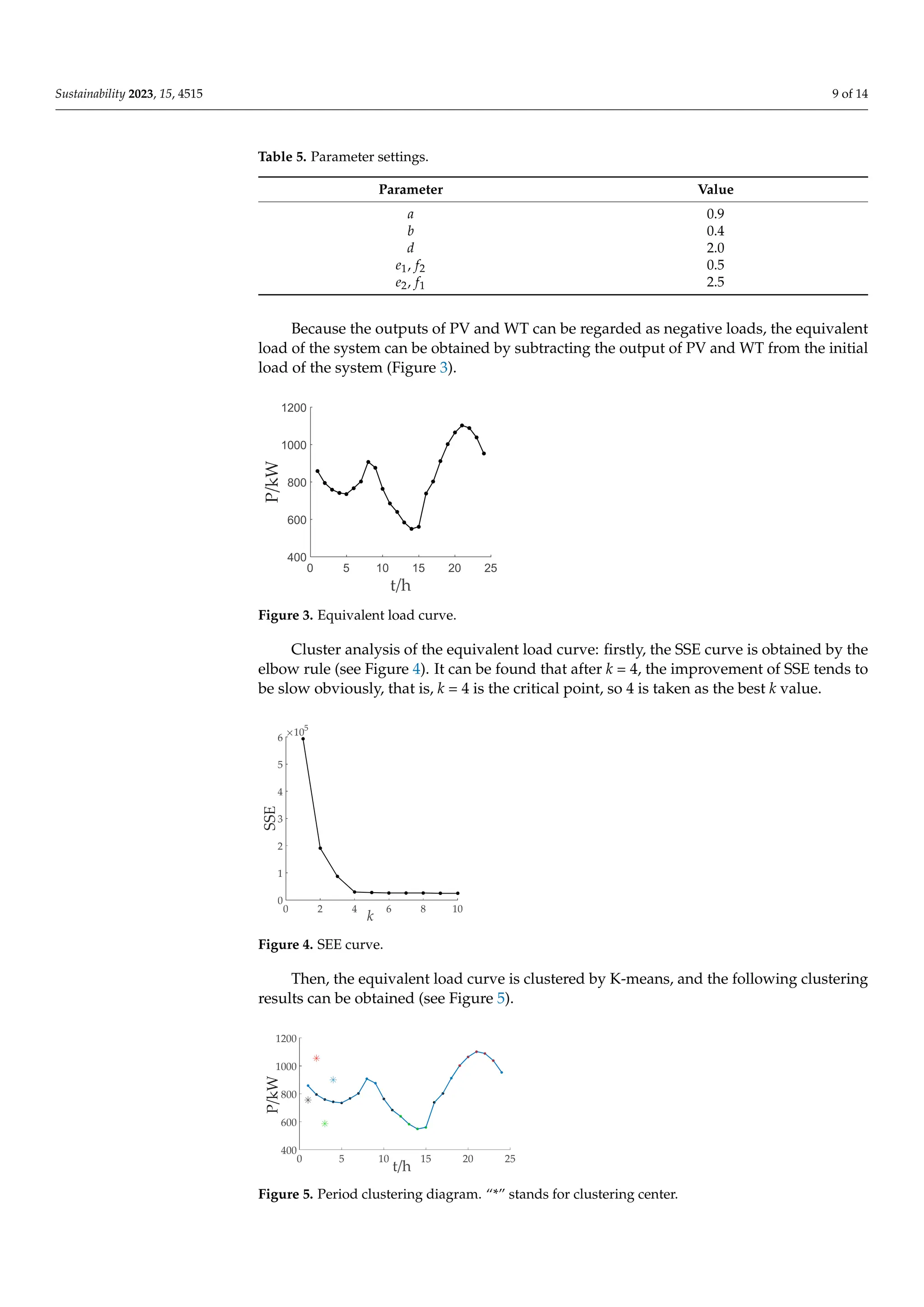
3.2. Elbow Rule Determines the Best Clustering Number k
The determination of clustering number k is very important to the clustering qual-
ity [25]. The larger the k value, the better the clustering effect, but the longer the calculation
time. The traditional k value is obtained through experience and lacks objectivity, so it is
necessary to choose the appropriate k value. In this paper, the elbow rule is adopted to
ensure the accuracy of k value selection. When Euclidean distance is used as the metric,
K-means takes the sum of squares for error (SSE) (also called the degree of distortion)
as the target to measure the clustering quality, and its calculation formula is shown in
Equation (19).
SSE = ∑
k
i=1 ∑p∈Ci
|p − mi|
2
(19)
where k represents the number of clusters; Ci represents the ith cluster; p represents the
sample point in Ci; and mi represents the mean value of all data in the ith cluster.
As the k value increases, the number of samples contained in each cluster decreases,
and the distance from the sample to its center will be closer, so the average distortion degree
will decrease [26]. For data with a certain degree of differentiation, when reaching a certain
critical point, the distortion degree will be greatly improved, and then slowly decreased,
and this critical point will be considered as the best k value.
3.3. Determination of Weighting Factor
In this paper, the PV output, WT output and load output of a day are superimposed
to obtain the equivalent load curve, and then the period of the equivalent load curve is
clustered, and then the fuzzy comprehensive evaluation method (FCE) is used to determine
the weighting factor of the optimization model in each period under the condition of
equivalent load [27]. Then, compare it with the weighting factor determined by the fixed
proportion method (FPM) (see Equation (22)) to establish two schemes for the weighting
factor. The calculation formula is as follows:
fn =
f 0
n
NF
∑
n=1
f 0
n
(20)
where f 0
n is the weighted value of exceeding the standard, calculated according to Equation (21);
and NF is the number of objective functions.
f 0
n =
Cn
Can,n
(21)
where Cn is actual value of the nth factor, n = 1, 2, 3; and Can,n is the maximum value of the
nth factor.
In this paper, Cn takes the average value of factors in each case, and Can,n takes the
maximum value of factors in each case.
fn =
1
NF
(22)
4. Solution of Mathematical Model
The particle swarm optimization (PSO) is used to solve the model established in this
paper. In PSO, multiple particles in the search space guide the update of speed and position
according to the global optimization and individual optimization, and co-evolve to find the
optimal solution of the problem [28]. The speed update equation is as follows [29]:
Vt+1
i,d = ωVt
i,d + r1c1(Pt
i,d − xt
i,d) + r2c2(Gt
i,d − xt
i,d) (23)](https://image.slidesharecdn.com/sustainability-15-04515-v31-240415040702-25ace7d3/75/stability-of-power-flow-analysis-of-different-resources-both-on-and-off-grid-6-2048.jpg)
![Sustainability 2023, 15, 4515 7 of 14
where Vt
i,d is the velocity of the ith particle in the tth iteration; r1 and r2, respectively,
represent random numbers evenly distributed in (0,1); c1 is a self-learning factor; c2 is a
global learning factor; and ω is the inertia weighting factor.
The location update formula is as follows:
Xt+1
i,d = Xt
i,d + Vt+1
i,d (24)
where Xt
i,d is the position of the ith particle in the tth iteration.
Considering the security of the power system, this paper gives the output constraints
of each unit to calculate the objective function value at each time. In order to avoid
the PSO algorithm falling into local optimization, this paper dynamically improves the
inertia weight ω and learning factors c1 and c2 [30,31], which are, respectively, shown in
Equations (25) and (26).
ω = a +
(a − b)gd
gd
max
(25)
where a and b are the maximum and minimum values of inertia weight ω; g is the current
iteration number; gmax is the maximum number of iterations; and d is a parameter.
c1 = (e1−e2)gd
gd
max
+ e2
c2 = (f1−f2)gd
gd
max
+ f2
(26)
where e1 and e2 are the maximum and minimum values of c1; f1 and f2 are the maximum
and minimum values of c2.
5. Analysis of Example
5.1. Basic Data
This paper simulates and analyzes the distribution network shown in Figure 1. ESS
is connected to 12 and 32 nodes; MG is connected to 3 and 24 nodes; PV is connected to
20 nodes; and WT is connected to 29 nodes. See Reference [6] for the network parameters.
Voltage reference value UB = 12.66 kV and power reference value SB = 1 MVA. The
specified voltage (per unit value) shall not be lower than 0.95 and not higher than 1.05; the
upper limit of the branch current is 20A; the upper limit of MG active output is 300 kW,
the lower limit is 100 kW, and the climbing speed Rdown, Rup is, respectively, −20 and
20 kW/h; and the maximum discharge power of the ESS is 250 kW, the maximum charging
power is 200 kW, and the self-discharge rate γ of the electric energy storage is 0.001. SOC0,
SOCmin, SOCmax is, respectively, 80, 40 and 160 kW · h. Select PV, WT and load data of
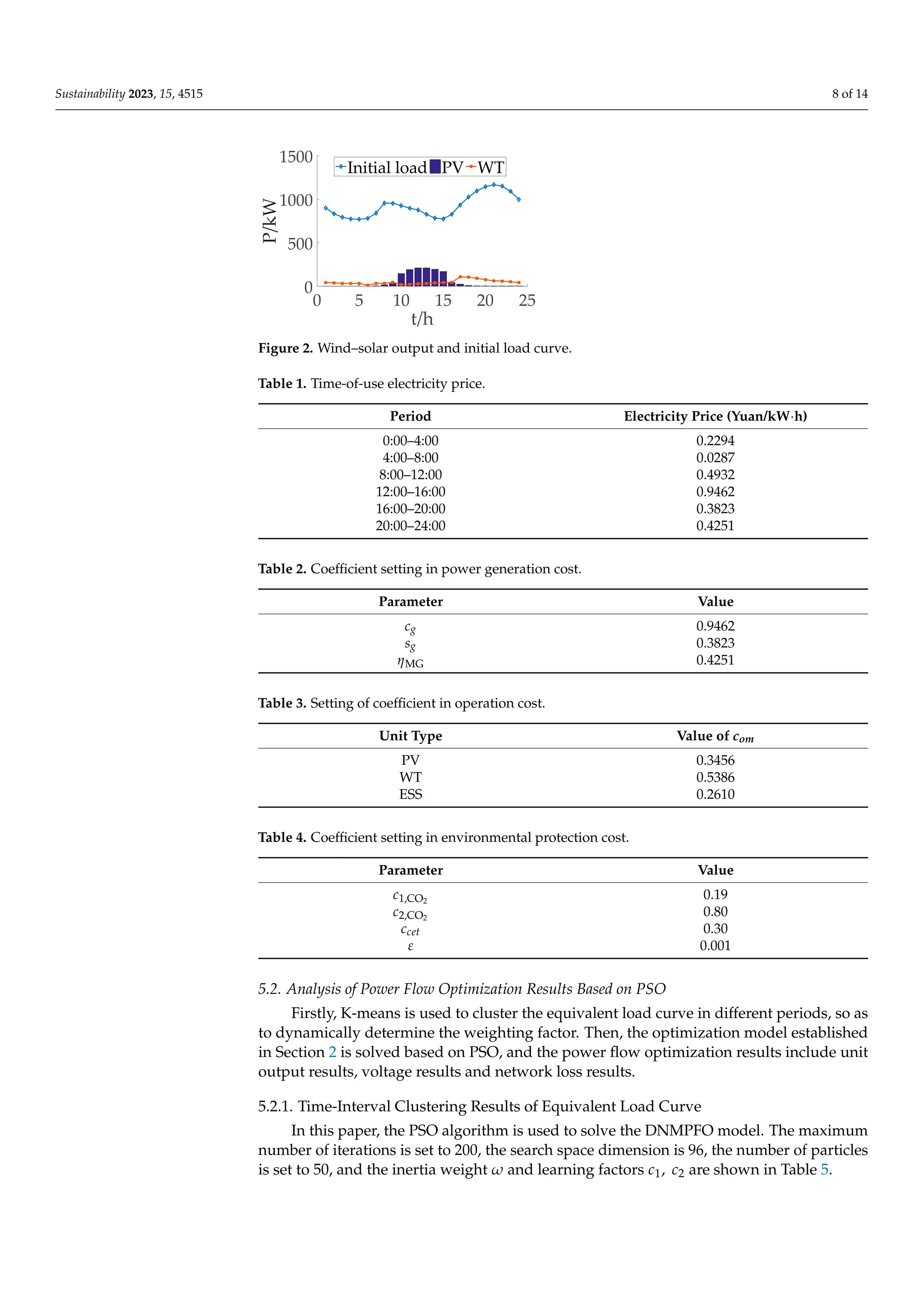
a certain area for analysis (see Figure 2). The time-of-use electricity price is shown in
Table 1. See Tables 2–4 for each cost coefficient in objective function F1. The DNMPFO
strategy based on the PSO algorithm proposed in this paper is used to optimize the power
flow of the distribution network for 24 h in this example to verify the effectiveness of the
proposed model.
Sustainability 2023, 15, x FOR PEER REVIEW 8 of 15
+
−
=
+
−
=
2
max
2
1
2
2
max
2
1
1
)
(
)
(
f
g
g
f
f
c
e
g
g
e
e
c
d
d
d
d
(26)
where 1
e and 2
e are the maximum and minimum values of 1
c ; 1
f and 2
f are the
maximum and minimum values of 2
c .
5. Analysis of Example
5.1. Basic Data
This paper simulates and analyzes the distribution network shown in Figure 1. ESS
is connected to 12 and 32 nodes; MG is connected to 3 and 24 nodes; PV is connected to
20 nodes; and WT is connected to 29 nodes. See Reference [6] for the network parame-
ters. Voltage reference value kV
66
12
= .
UB and power reference value MVA
1
=
B
S .
The specified voltage (per unit value) shall not be lower than 0.95 and not higher than
1.05; the upper limit of the branch current is 20A; the upper limit of MG active output is
300kW, the lower limit is 100kW, and the climbing speed down
R
, up
R
is, respectively,
−20 and 20 kW/h ; and the maximum discharge power of the ESS is 250 kW, the maxi-
mum charging power is 200 kW, and the self-discharge rate γ
of the electric energy
storage is 0.001. 0
SOC
, min
SOC
, max
SOC
is, respectively, 80, 40 and 160 h
kW ⋅ . Se-
lect PV, WT and load data of a certain area for analysis (see Figure 2). The time-of-use
electricity price is shown in Table 1. See Tables 2–4 for each cost coefficient in objective
function 1
F
. The DNMPFO strategy based on the PSO algorithm proposed in this paper
is used to optimize the power flow of the distribution network for 24 h in this example
to verify the effectiveness of the proposed model.
Figure 1. IEEE33 node radial distribution network system diagram. “1, 2, 3” stands for nodes, and
“(1), (2), (3) stands for branches.
500
1000
1500
Initial load PV WT
Figure 1. IEEE33 node radial distribution network system diagram. “1, 2, 3” stands for nodes, and
“(1), (2), (3) stands for branches.](https://image.slidesharecdn.com/sustainability-15-04515-v31-240415040702-25ace7d3/75/stability-of-power-flow-analysis-of-different-resources-both-on-and-off-grid-7-2048.jpg)
![Sustainability 2023, 15, 4515 13 of 14
6. Conclusions
In this paper, the DNMPFO model is established, and the model is solved by PSO
algorithm. The effectiveness of this method is verified based on an IEEE33-bus system. The
conclusions are as follows.
(1) When establishing the DNMPFO model, taking the lowest total cost, the lowest voltage
deviation and the lowest power loss including fuel cost, operation and maintenance
cost, power purchase cost and pollutant emission control cost as objective functions,
and comprehensively considering multiple constraints such as power flow constraint,
climbing constraint and energy storage operation constraint, it can be more in line
with the actual operation situation of distribution network, and the comprehensive
optimization effect is better;
(2) K-means clustering is used to divide the equivalent load after the superposition of
PV, WT and load output for 24 h a day into different periods, and FCE is used to
dynamically determine the weighting factor of each period, so that the determination
of the weighting factor is more reasonable and the subsequent optimization effect
is better;
(3) The results of PSO algorithm show that the calculation results of this strategy can
effectively reduce the economic cost, improve the voltage deviation and reduce the
power loss, thus improving the economy and reliability of power grid operation.
Author Contributions: Conceptualization, F.Z. and X.M.; methodology, X.M.; software, F.Z.; val-
idation, F.Z., X.M. and L.W.; formal analysis, X.M.; investigation, L.W. and N.Z.; resources, L.W.;
data curation, N.Z.; writing—original draft preparation, F.Z.; writing—review and editing, X.M.;
visualization, N.Z.; supervision, X.M.; project administration, N.Z.; funding acquisition, N.Z. All
authors have read and agreed to the published version of the manuscript.
Funding: This research was funded by Youth Program of National Natural Science Foundation of
China (Grant number 61903264).
Informed Consent Statement: Informed consent was obtained from all subjects involved in
the study.
Data Availability Statement: Not applicable.
Conflicts of Interest: The authors declare no conflict of interest.
References
1. Zhao, M.; Hengxu, Z.; Haoran, Z.; Mengxue, W.; Yuanyuan, S. New mission and challenge of power distribution and consumption
system under dual-carbon target. Proc. CSEE 2022, 42, 6931–6945.
2. Zhigang, Z.; Chongqing, K. Challenges and prospects for constructing the new-type power system towards a carbon neutrality
future. Proc. CSEE 2022, 42, 2806–2819.
3. Xiping, M.; Rong, J.; Chen, L.; Weizhou, W.; Rui, X. Review of researches on loss reduction in context of high penetration of
renewable power generation. Power Syst. Technol. 2022, 46, 4305–4315.
4. Chengzhou, L.; Ligang, W.; Yumeng, Z.; Hangyu, Y.; Zhuo, W.; Liang, L.; Ningling, W.; Zhiping, Y.; Maréchal, F.; Yongping, Y. A
multi-objective planning method for multi-energy complementary distributed energy system: Tackling thermal integration and
process synergy. J. Clean. Prod. 2023, 390, 135905. [CrossRef]
5. Zhonghui, Z.; Dayong, L.; Jun, L.; Yanyu, X.; Junwei, X. Source-network-load-storage bi-level collaborative planning model of
active distribution network with sop based on adaptive ε-dominating multi-objective particle swarm optimization algorithm.
Power Syst. Technol. 2022, 46, 2199–2212.
6. Mengyi, L.; Xiaoyan, Q.; Zhirong, Z.; Changshu, Z.; Youlin, Z. Multi-objective reactive power optimization of distribution network
considering output correlation between wind turbines and photovoltaic units. Power Syst. Technol. 2020, 44, 1892–1899.
7. Chunyan, L.; Chenyu, Z.; Bo, H.; Zhengyu, C.; Qinglong, L. Two-stage clustering algorithm of typical wind-PV-load scenario
generation for reliability evaluation. Electr. Eng. Energy 2021, 40, 1–9.
8. Lili, W.; Hao, W.; Zhouyang, R.; Yihao, S. Evaluation of renewable energy accommodation capacityof high voltage distribution
networks considering regulation potential of flexible resources. Electr. Power 2022, 55, 124–131.
9. Huankun, Z.; Fanfei, Z.; Yu, F.; Chaochao, H.; Lingyu, Z. Bi-level distributed power planning based on e-c-k-means clustering
and sop optimization. Acta Energ. Sol. Sin. 2022, 43, 127–135.](https://image.slidesharecdn.com/sustainability-15-04515-v31-240415040702-25ace7d3/75/stability-of-power-flow-analysis-of-different-resources-both-on-and-off-grid-13-2048.jpg)
![Sustainability 2023, 15, 4515 14 of 14
10. Jiaxin, G.; Jing, B.; Guoqing, L.; He, W. Wind power fluctuation considered calculation of interval optimal power flow in AC/DC
system and configuration of DCPFC. Mod. Electr. Power 2020, 37, 613–623.
11. Sachin Sharma, K.; Niazi, R.; Kusum, V.; Tanuj, R. Coordination of different DGs, BESS and demand response for multi-objective
optimization of distribution network with special reference to Indian power sector. Int. J. Electr. Power Energy Syst. 2020,
121, 106074. [CrossRef]
12. Zhao, H.; Pengbo, M.; Mengmeng, W.; Baling, F.; Ming, Z. A Hierarchical Strategy for Multi-Objective Optimization of Distribution
Network Considering DGs and V2G-Enabled EVs Integration. Front. Energy Res. 2022, 10, 869844.
13. Yang, X.; Wang, L. Optimization of distributed power distribution network based on probabilistic load flow. Acta Energ. Sol. Sin.
2021, 42, 71–76.
14. Qifen, L.; Yihan, Z.; Yongwen, Y.; Liting, Z.; Chen, J. Demand-Response-Oriented Load Aggregation Scheduling Optimization
Strategy for Inverter Air Conditioner. Energies 2022, 16, 337. [CrossRef]
15. Guan, W.; Zhongfu, T.; Qingkun, T.; Shenbo, Y.; Hongyu, L.; Xionghua, J.; De, G.; Xueying, S. Multi-Objective Robust Scheduling
Optimization Model of Wind, Photovoltaic Power, and BESS Based on the Pareto Principle. Sustainability 2019, 11, 305. [CrossRef]
16. Al-Kaabi, M.; Dumbrava, V.; Eremia, M. Single and Multi-Objective Optimal Power Flow Based on Hunger Games Search with
Pareto Concept Optimization. Energies 2022, 15, 8328. [CrossRef]
17. Zailin, P.; Xiaofang, M. Distribution Network Planning; Electric Power Press: Beijing, China, 2015; pp. 180–197.
18. Jun, D.; Zongnan, Z.; Menghan, L.; Jing, G.; Kongge, Z. Optimal scheduling of integrated energy system based on improved grey
wolf optimization algorithm. Sci. Rep. 2022, 12, 1–19.
19. Rauf, A.; Kassas, M.; Khalid, M. Data-Driven Optimal Battery Storage Sizing for Grid-Connected Hybrid Distributed Generations
Considering Solar and Wind Uncertainty. Sustainability 2023, 14, 110002. [CrossRef]
20. Ciwei, G.; Wei, W.; Tao, C. Capacity Planning of Electric-hydrogen Integrated Energy Station Based on Reversible Solid Oxide
Battery. Proc. CSEE 2022, 42, 6155–6170.
21. Yanbo, C.; Yanhu, M.; Guodong, Z.; Zhixiang, S.; Donghui, C. Coordinated planning of thermo-electrolytic coupling for multiple
chp units considering demand response. Power Syst. Technol. 2022, 46, 3821–3832.
22. Shouxiang, W.; Qi, L.; Qianyu, Z.; Zhuoran, L.; Kai, W. Improved particle swarm optimization algorithm for multi-objective
voltage optimization of ac/dc distribution network considering the randomness of source and loads. Proc. CSU-EPSA 2021, 33,
10–17.
23. Zhaolong, Z.; Shaishai, Z.; Bo, Z. A fast classification method based on factor analysis and K-means clustering for retired electric
vehicle batteries. Power Syst. Prot. Control 2021, 49, 41–47.
24. Fangfang, Z.; Xiaofang, M.; Lidi, W.; Nannan, Z. Operation Optimization Method of Distribution Network with Wind Turbine
and Photovoltaic Considering Clustering and Energy Storage. Sustainability 2023, 15, 2184. [CrossRef]
25. Yang, H.; Qian, L.; Fang, F.; Yuchen, H. Dynamic interval modeling of ultra-short-term output of wind farm based on finite
difference operating domains. Power Syst. Technol. 2022, 46, 1346–1357.
26. Changjuan, L.; Yunlong, C.; Jiyan, L.; Xuemei, Z.; Xiaoyu, W. Ensemble learning-based day-ahead power forecasting of distributed
photovoltaic generation. Electr. Power 2022, 55, 38–45.
27. Xiaofang, M.; Lidi, M.; Xiaoning, W.; Yingnan, W.; Ran, L. Improve operation characteristics in three-phase four-wire low-voltage
distribution network using distributed generation. Power Syst. Technol. 2018, 2018, 4091–4100.
28. Xiaojuan, L.; Jianjun, W.; Yuen, C.W.; Qian, L. Multi-objective Intercity Carpooling Route Optimization Considering Carbon
Emission. Sustainability 2023, 15, 2261. [CrossRef]
29. Shuqin, S.; Chenyue, W.; Wenli, Y.; Mingnan, L.; Yujie, L. Optimal power flow calculation method based on random attenuation
factor particle swarm optimization. Power Syst. Prot. Control 2021, 49, 43–52.
30. Zhen, S.; Xiaosong, Z.; Xufeng, Y.; Wei, X.; Yong, Y. Optimization of peak load shifting in distribution network based on improved
mopso algorithm. Sci. Technol. Eng. 2020, 20, 3984–3989.
31. Yunhao, H.; Wu, Z.; Yiqi, J.; Shixuan, W. Research on photovoltaic mppt control based on adaptive mutation particle swarm
optimization algorithm. Acta Energ. Sol. Sin. 2022, 43, 219–225.
Disclaimer/Publisher’s Note: The statements, opinions and data contained in all publications are solely those of the individual
author(s) and contributor(s) and not of MDPI and/or the editor(s). MDPI and/or the editor(s) disclaim responsibility for any injury to
people or property resulting from any ideas, methods, instructions or products referred to in the content.](https://image.slidesharecdn.com/sustainability-15-04515-v31-240415040702-25ace7d3/75/stability-of-power-flow-analysis-of-different-resources-both-on-and-off-grid-14-2048.jpg)