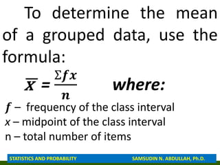
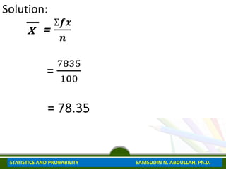
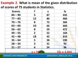
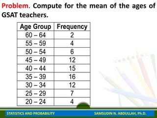
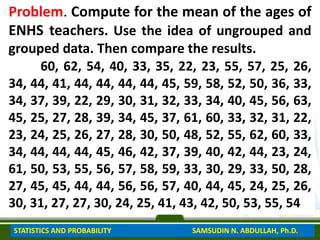
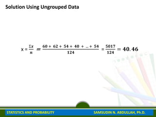
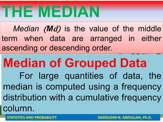
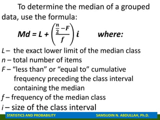
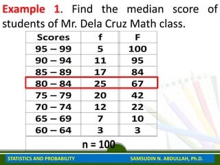
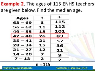
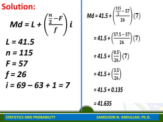
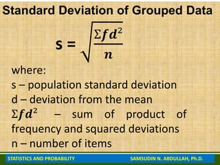
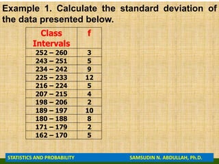
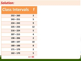
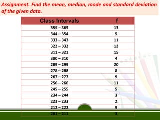
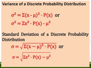
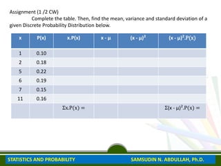
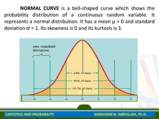
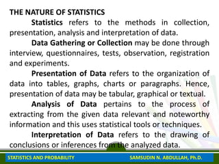
The document discusses measures of central tendency and variability in statistics and probability. It provides definitions and formulas for calculating the mean, median, mode, range, standard deviation, and variance of both ungrouped and grouped data. Examples are given to demonstrate calculating the mean and median of frequency distributions. The key information is that the document outlines statistical concepts and formulas for central tendency and variability and provides examples to show how to apply these formulas.


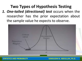
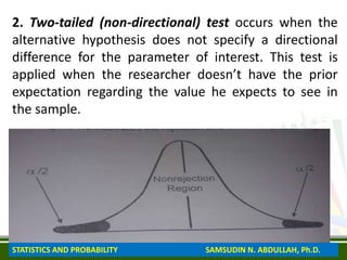


![MEASURES-OF-CENTRAL-TENDENCIES-1[1] [Autosaved].pptx](https://cdn.slidesharecdn.com/ss_thumbnails/measures-of-central-tendencies-11autosaved-220906145428-d730d0eb-thumbnail.jpg?width=640&height=640&fit=bounds)


