The document discusses statistical inference and hypothesis testing, illustrating how sample statistics can estimate population parameters and the methodologies for testing hypotheses. It covers concepts such as probability distributions, normal distributions, interval estimation, and hypothesis testing in various scenarios, including bivariate regression. The document emphasizes the importance of confidence intervals and significance levels in making statistical conclusions.

1. Statistical Inference
and
Hypothesis Testing

2. Why ?
• Samples drawn from an infinite population
• Features of population may vary from those of
samples
• Sample statistics may vary with samples
• Question is whether the sample properties
satisfactorily explain population properties
• Parameter -> population characteristics (mean,
variance etc.)
• Statistic -> sample characteristics

3. Statistical Inference
• Statistical inference The process of going to
unknown population parameters from estimated
sample statistics possible with random
sampling
• 2 problems -> no idea about the feature of the
population – estimation, then testing of
hypothesis
• -> tentative idea about the feature of the
population – testing of hypothesis

4. Estimation
• Interval estimation -> a range of values within which
the unknown parameter has a chance to belong
• Point estimation -> estimate a particular value for
the unknown parameter – test whether the
estimation is satisfactory/ reliable – hypothesis
testing
• Testing reliability (whether statistically significant) of
estimation needs knowledge of probability
distribution function

5. Probability
• Probability of an event = (Number of cases
favourable to the event) / (Total number of cases)
• Example: Coin tossing (2 times)
• Events: HH, HT, TH, TT
• Probability (Different outcomes) = 2/ 4
• In axiomatic approach of probability relative
frequency of an event is considered as the event’s
probability of occurrence when the total number of
cases is very large (n -> ∞)

6. Probability distribution
• Y is a random variable => Y occurs with probability
• As probability is defined by relative frequency,
distribution of Y in the infinite population is
represented by its probabilities => Probabilities of
occurrence of different values of Y are presented
against those values of Y
• Y is discrete -> for any particular value of Y (let it be
c), f(c) = f(Y at c)= Pr(Y=c)
• f(Y) is the pmf (probability mass function) of Y if
• f(Y) ≥ 0, for any Y
• ∑ f(Y) = 1, summation with all values that Y can
assume

7. Probability distribution
• Y is continuous -> for two values of Y, a (lower) and b
(upper),
b
• Pr(a≤Y≤b) = ∫ f(Y)dY
a
• f(Y) is the pdf (probability density function) of Y if
• f(Y) ≥ 0, for any Y
∫ f(Y)dY = 1, integration for all values of Y, (-∞, +∞)

8. Distribution function
• Statistical inference involves inferring the nature of a
population (central tendency - mean, variance,
skewness and kurtosis) from the nature of a sample
• -> we take help of distribution function
• For any value c of the continuous variable Y,
c
• F(c) = Pr( Y ≤ c)) = ∫ f(Y)
-∞
is called the cumulative distribution function or
distribution function of Y

9. Theoretical distribution
• -> f (a theoretical distribution) gives a fairly
close approximation to the actual distribution
of the population variable
• -> inference problem is related to having an
idea about the numerical values of (or
estimate) the parameters appearing in f
• -> We have an idea regarding the central
tendency of the variable concerned from its
theoretical distribution (mean, variance etc.)

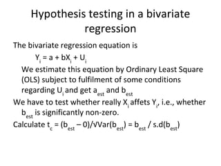
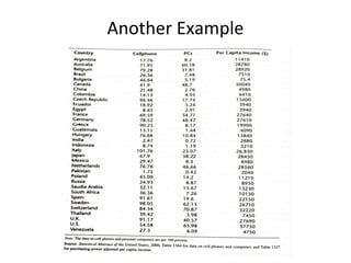
10. Normal Distribution
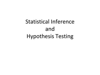
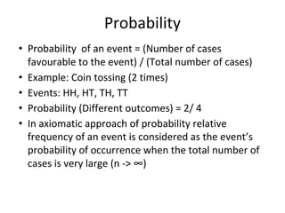
• Most used form of distribution for a continuous
variable because
• – has very simple properties – comparatively easy to
deal with
• - many non-normal distributions become
asymptotically normal
• - transformation of variables often make them follow
normal distribution
• Central limit theorem and law of large numbers
• f(Y) = (1/(σ√2π) exp[-(Y-μ)2
/2σ2
], -∞ ≤Y ≤ +∞
• Mean(Y) = μ, Var(Y)= σ2

11. Normal Distribution

12. Properties of normal distribution
f(Y) > 0 for all values of Y
∞
∫ f(Y)dY = 1
-∞
The distribution is symmetrical
=> mean and median are the same
Any linear function of some normal variables is also
normally distributed.
=> If Y1
, Y2
, Y3
are normally distributed, (Y1
+ Y2
+ Y3
)/3
is also normally distributed

13. Normal Distribution Standard
Normal Distribution
• Population distribution Sampling distribution
• Population (Mean, Variance) Sample (Mean,
Variance)
• Distribution of the sample is also normal
• If Y follows normal distribution with mean = μ and
variance = σ2
, then
τ = (Y- μ)/ σ follows standard normal distribution
with Mean = 0 and variance = 1

14. Standard Normal Distribution

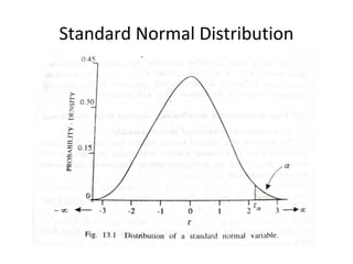
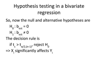
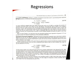
15. Statistical Inference
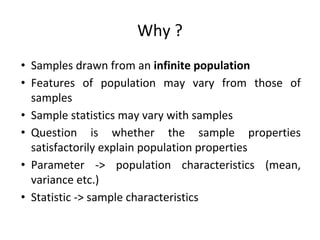
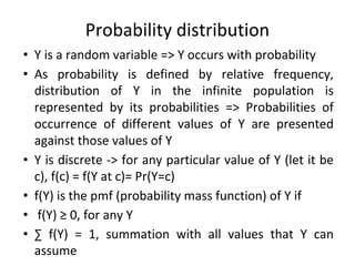
Let us denote by τα,
a value of τ, such that
Pr[τ > τα
] = α
and Pr[τ < τ1-α
] = α
⇒ Pr[τ < τα
] = 1-α
For statistical inference value of α is normally
considered as 0.01 (99 per cent) or 0.05 (95 per cent)
and Pr[ -τα/2
< τ < τα/2
] = 1-α
The interval is defined as confidence limit and (1-α) is
confidence coefficient

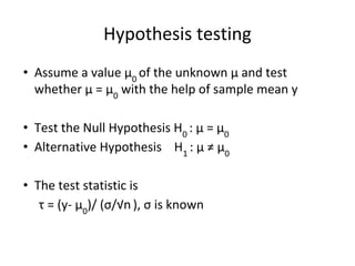
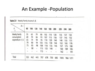
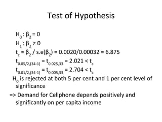
16. Interval estimation
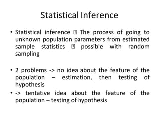
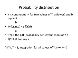
• Constructing a range of values (interval) within which
the unknown parameter has a chance to belong
• If y is sample mean (samples being y1
, y2
, ......., yn
), it
can be shown that E(y) = μ, Var(y)= σ2
/n (sampling
with replacement)
• If y1
, y2
, ......., yn
follow normal distribution, y also
follows normal distribution
• Define τ = (y- μ)/ (σ/√n ), τ = [y- Mean(y)]/ √Var(y),
• τ follows standard normal distribution

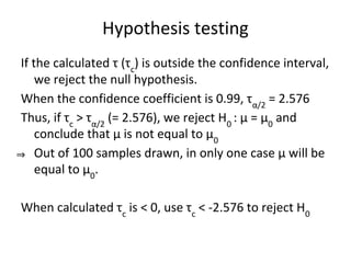
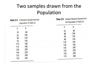
17. Interval estimation
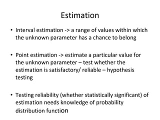
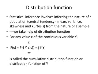
99 per cent confidence interval of μ is
Pr [-2.576 ≤ (y- μ)/ (σ/√n ) ≤2.576] = 0.99
Pr [-2.576 (σ/√n ) ≤ (y- μ) ≤2.576 (σ/√n )] = 0.99
Pr [- y- 2.576 (σ/√n ) ≤ - μ ≤ -y +2.576 (σ/√n )] = 0.99
=> Pr [y- 2.576 (σ/√n ) ≤ μ ≤ y +2.576 (σ/√n )] = 0.99
=> In repeated sampling, in 99 per cent of the cases the
above interval will include μ (the probability that the
above interval will include μ is 0.99)

18. Hypothesis testing
• Assume a value μ0
of the unknown μ and test
whether μ = μ0
with the help of sample mean y
• Test the Null Hypothesis H0
: μ = μ0
• Alternative Hypothesis H1
: μ ≠ μ0
• The test statistic is
τ = (y- μ0
)/ (σ/√n ), σ is known

19. Hypothesis testing
If the calculated τ (τc
) is outside the confidence interval,
we reject the null hypothesis.
When the confidence coefficient is 0.99, τα/2
= 2.576
Thus, if τc
> τα/2
(= 2.576), we reject H0
: μ = μ0
and
conclude that μ is not equal to μ0
⇒ Out of 100 samples drawn, in only one case μ will be
equal to μ0
.
When calculated τc
is < 0, use τc
< -2.576 to reject H0

20. If the null hypothesis is H0
: μ = μ0
against the alternative H1
: μ > μ0
or H1
: μ < μ0
we choose one-sided critical value, τα,
instead of τα/2
Here the critical (tabulated) value will be 2.326

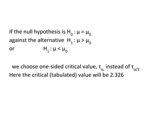
21. t-distribution
• When σ is unknown, it is replaced by its sample
estimate.
• Then the ratio [(y-mean)/std. dev] follows
t-distribution
• The (1-α) percent confidence interval is
Pr [y- tα/2,n-1
(s’/√n ) ≤ μ ≤ y + tα/2,n-1
(s’/√n )] = 1-α

22. Hypothesis testing in a bivariate
regression
The bivariate regression equation is
Yi
= a + bXi
+ Ui
We estimate this equation by Ordinary Least Square
(OLS) subject to fulfilment of some conditions
regarding Ui
and get aest
and best
We have to test whether really Xi
affets Yi
, i.e., whether
best
is significantly non-zero.
Calculate tc
= (best
– 0)/√Var(best
) = best
/ s.d(best
)

23. Hypothesis testing in a bivariate
regression
So, now the null and alternative hypotheses are
H0
: best
= 0
H1
: best
≠ 0
The decision rule is
if tc
> tα/2,(n-1)
, reject H0
=> Xi
significantly affects Yi

24. An Example -Population

25. Two samples drawn from the
Population

26. Two SRFs estimated from Two
Samples

27. Another Example

28. Regressions

29. Test of Hypothesis
H0
: β2
= 0
H1
: β2
≠ 0
tc
= β2
/ s.e(β2
) = 0.0020/0.00032 = 6.875
t0.05/2,(34-1)
= t0.025,33
= 2.021 < tc
t0.01/2,(34-1)
= t0.005,33
= 2.704 < tc
H0
is rejected at both 5 per cent and 1 per cent level of
significance
=> Demand for Cellphone depends positively and
significantly on per capita income