The document is a comprehensive statistics formula sheet detailing various statistical concepts including measures of central tendency, probability, sampling, quality control, and index numbers. It presents formulas for calculating means (arithmetic, geometric, harmonic), standard deviations, regression models, correlation coefficients, and several probability rules. Additionally, it includes methods for interpolation, extrapolation, and time series analysis, along with control chart parameters for quality control.

1. Stat 101
Formulae Sheet
MMM, Histogram, Central Tendency
Name
Sl.no.
1.
Relative Frequency
3.
l
m
Midpoint
2.
Formula
Angle of Pie
s
2
RF= proportion=
0
f
* 360
0
N
U
4.
Mean ( )
G
n
Me
L0
F
2
Me
* W Me
f Me
Me
5.
Median (Me)
Median
L0
Lower Limit of the median
class
W Me
Width of the median
class
CF of the pre median class
n
Total number
G
F
F of the median class
U
6.
7.
Me
f Me
Mode (M0)
11304042
Classic way- count the middle value
U
The number with the most frequency
Page 1

2. 9.
10.
Mode
Lower Limit of Modal class
f0
G
Mo
L0
8.
F of the modal class
f
F of the pre modal class
1
F of post modal class
f1
Width of the modal class
W
U
Geometric Mean
(GM)
1
G
f
GM
f
f
x 1 1 . x 2 2 ... x k k
n
1
...
Weighted Mean (
14.
fi
HM
Coefficient of Range
(Co. R)
17.
Quartile Deviation
(QD)
f1
f2
xi
n
n
fk
x2
...
xk
W1 X 1
WX
Xw
Range (R)
16.
1
W2 X 2
fi
i 1
...
xi
Wn X n
Quartile (Q)
15.
i 1
i 1
x1
13.
f i log x i
i 1
k
G
12.
1
x2
Harmonic Mean (HM)
k
n
n
xn
1
x1
11.
1
anti log
n
HM
U
GM
n
11304042
)
W
W1
R
W2
A
(Q 2
Q1 )
Xl
X
s
Xl
QD
X
s
(Q 3
2
Wn
Xs.
Xl
Coeff .. R
...
Q2 )
R
Q3
Q1
A
2
Page 2

3. 18.
19.
20.
21.
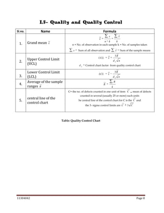
Coeff.
Coefficient of QD
U
Mean Deviation (MD)
Where A can be mean/
median/mode
1
MD
Population
i
1
i
2
i
1
N
R
2
Sample
1
i
k
1
i
i
1
23.
1
N
1
2
2
k
1
s
n
1
2
n
f 1 x1
k
1
Ungroup data
22.
i
2
fi xi
N
fi x
i
Sample
n
2
xi
2
f 1 x1
xi
N
1
2
fi Di
N
k
i
N
s
A =
A
1
Population
x
Di
N
Group data
x
N
1
2
N
1
R
Coeff. MD =
Ungroup data
N
A =
fi X i
N
Coefficient of MD
2
Q1
Xi
N
G
Q1
Q3
1
MD
Q3
QD
2
i
i
1
1
n
Group data
Standard Deviation
SD X
[SD(X)]
Coefficient of
VAR X
CV
Variation (CV)
VAR(X) =
=
SD ( X )
2
/ s2
A
.
R
AM ( X )
Mean
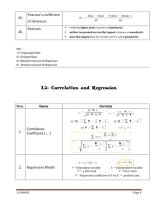
Skewness
11304042
Mode
The distribution is positively skewed
Mean
Median
Mode
The distribution is negatively skewed
Mean
24.
Median
Median
Mode
The distribution is symmetric
Page 3

4. 25.
Pearson’s coefficient
Sk
of skewness
Mean
p
3 ( Mean
Mode
SD
Median )
SD
relatively higher peak is known as leptokurtic.

neither too peaked nor too flat topped is known as mesokurtic.

26.

Kurtosis
more flat topped than the normal curve is called platykurtic.
Key:
U= Ungrouped Data
G= Grouped Data
A= Absolute measure of Dispersion
R= Relative measure of Dispersion
L2- Correlation and Regression
Name
Sl.no.
Formula
SP X , Y
r xy
SP XY
1.
Correlation
Coefficient ( r xy )
X
i
SS Y
X Yi
Yi
Y
rxy
X
Y
2.
Regression Model
11304042
Y
X
Xi
n
V
,
X ,Y
X V Y
SS X
2
Y
Xi
1
Xi
X iYi
2
i
Cov
r xy
SS X SS Y
rxy
X
2
1
Yi
n
2
Yi
Yi
2
2
n
ˆ
Yi
ˆ
ˆX
X Independent variable
Dependent variable
Intercept
Error term
Y
Regression coefficient of Y on X
gradient (m)
Page 4

5. 3.
4.
least square method
&
are the parameters of the model.
Estimating the
regression
ˆ
n
X iYi
n
coefficient
2
Xi
Xi
Yi
X iYi
ˆ
2
Xi
X
2
i
nXY
nX
2
Estimating the
intercept
ˆ
:
ˆX
Y
L3- Probability
Name
Sl.no.
3.
11304042
rule
2.
Empirical or Frequency
Probability
ion
Classic Probability
Addit
1.
Formula
General Case
P A
m
;
n
P A
m
lim
m
n
No. of times event A occurs. n
P AorB
P ( A)
P(B)
;
n
Total no. of trials.
P ( AandB )
Page 5

6. ( NOT mutually exclusive)
P A
B
P ( A)
Special case
( mutually exclusive)
5.
6.
Multiplication
4.
P AorB
P A
P ( AB )
Independent events
Events that are not independent
P(B)
P ( A)
B
P(A
P(B)
P ( A)
B)
P ( AB )
P(B)
P ( A) P ( B )
conditional probability of A given B
P ( AB )
P(A B)
; P(B) 0
P(B)
conditional probability of B given A
P ( AB )
P ( B A)
; P ( A) 0
P ( A)
L4- Sampling
Name
1.
2.
3.
4.
5.
Perc
Simple Random Sampling
enta
ge
Standard
stan
error of
dard
erro
r of
Sl.no.
11304042
estimate of Population Mean Est Y
estimate of population total Est
the estimate of Population
Mean SE ( y )
the estimate of Population
Total Est SE ( N y )
Estimate of Population mean
SE ( y ) %
Formula
n
Y
ˆ
Y
yi
i 1
y
n
NY
SE ( y )
ˆ
NY
Ny
N
n
s
2
Nn
SE ( N y )
SE ( y )
N * SE ( y )
SE ( y )
* 100
y
Page 6

7. 6.
* 100
Ny
s
y
n
1
2
n
Sample Variance s2
7.
SE ( N y )
SE ( N y )
Estimate of Population total %
2
yi
1
ny
2
i 1
Sample Mean, N = Population size
12.
13.
14.
15.
16.
17.
18.
19.
11304042
Standard
error of
Percentage
standard error
of
11.
ˆ
Y
Y
estimate of population Total Est
the estimate of Population
Mean SE ( y st )
the estimate of Population
Total Est SE ( N y st )
Estimate of Population mean
SE ( y st ) %
Estimate of Population total %
n
NY
N y st
2
the estimate of Population
Mean SE ( y sys )
ni
N
the estimate of Population
Total Est SE ( N y sys )
Estimate of Population mean
SE ( y sys ) %
Estimate of Population total %
SE ( N y sys )
2
W i si
N * SE ( y st )
SE ( y st )
SE ( y st )
* 100
y st
SE ( N y st )
SE ( N y st )
* 100
N y st
ˆ
Y
1
y sys
NY
SE ( y sys )
2
1
SE ( N y st )
estimate of population Total Est
Wi yi
i 1
W i si
SE ( y st )
Y
k
1
y st
SE ( N y st )
estimate of population Mean Est
Standard
error of
10.
estimate of population Mean Est
Percentage
standard error
of
9.
Systematic Random Sampling
8.
Stratified Random Sampling
and n = Sample size
N y sys
1
m (m
SE ( N y sys )
SE ( y sys )
SE ( N y sys )
yj
m
1)
yj
y sys
N * SE ( y sys )
SE ( y sys )
* 100
y sys
SE ( N y sys )
* 100
N y sys
Page 7
2

8. L5- Quality and Quality Control
Name
Sl.no.
Formula
x
x
x
1.
Grand mean
n k
k
n = No. of observation in each sample k = No. of samples taken
x
x
2.
3.
4.
5.
Upper Control Limit
(UCL)
UCL
d2
Sum of the sample means
x
3R
x
d2
Lower Control Limit
(LCL)
Average of the sample
ranges R
central line of the
control chart
Sum of all observation and
n
Control chart factor from quality control chart
LCL
3R
x
d2
n
R
R
k
C= the no. of defects counted in one unit of item C = mean of defects
counted in several (usually 25 or more) such units
he central line of the control chart for C is the C and
the 3- sigma control limits are C
3 C
Table: Quality Control Chart
11304042
Page 8

9. Interpolation & Extrapolation
yx
6.
y0
u y0
u u
1
2
2!
Newton’s Forward
interpolation
formulae y x
u u
y0
2
3
3!
x
u
1 u
y0
...
...
...
x0
h
x= the value of x for which the value of y is to be determined
h=common intervals between x values
7.
Newton’s Back ward
interpolation
formulae
11304042
yx
yn
u
1
yn
u u
1
2
2!
u
u u
yn
1 u
3!
x
2
3
yn
...
xn
h
Page 9
...
...

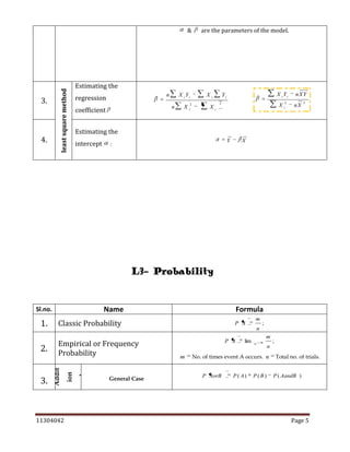
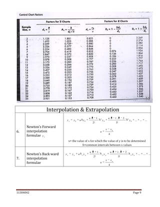
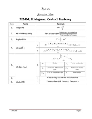
10. L5- Index Number
Name
Sl.no.
1.
Un-weighted Index
Numbers (Simple
Aggregative Method)
Formula
2.
Total of base year prices for various commodities
P
1
* 100
P
0
N
P
01
Where N refers to no. of items
log[
P
1
* 100 ]
P
0
log P
01
log P
or
N
Where
3.
* 100
P0
Total of current year prices for various items
P1
P0
Un-weighted Index
Numbers (Simple
Average Relative of
Method)
P1
P01
P01
Laspeyres Method
N
P1
P
* 100
P2
PQ
1 0 * 100
P Q
0 0
Weight is Base year quantity
4.
P
01
Paasche Method
PQ
1 1
* 100
P Q
0 1
Weight is Current year quantity
5.
6.
Dorbish and Bowley’s
Method
P1 Q 0
[Where L
Fisher’s ‘Ideal’ Method
8.
Marshall – Edgeworth
Method
Kelly’s Method
P
01
P
P0 Q 1
2
P1Q 0
L*P
Paasche Index]
P1Q1
*
P0 Q 0
(Q 0
Q1 ) P1
(Q 0
Q1 ) P0
Paasche Index]
P1Q 0
P1Q
P1Q1
P0 Q 0
* 100
P
01
* 100
P0 Q1
Laspeyres Index and P
[Where Q
11304042
* 100
2
Lasperes Index and P
P
01
[Where L
7.
L
P
01
P1 Q 1
P0 Q 0
P0 Q1
* 100
* 100
P0 Q
Q0
Q1
2
]
Page 10

11. L5- Time Series Analysis & Forecasting
Sl.no.
11304042
Name
Formula
Page 11