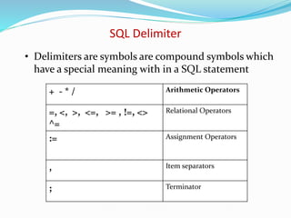
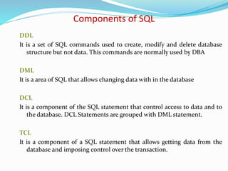
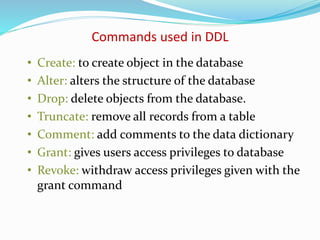
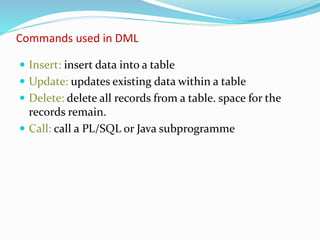
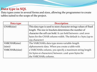
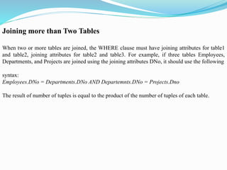
SQL is a standardized programming language used to manage and manipulate relational databases, supporting operations like data definition, data manipulation, and transaction control. It allows users to perform various commands such as creating, modifying, and deleting tables, as well as managing data access and executing transactions. SQL uses an English-like syntax and includes essential components like operators and data types to facilitate these tasks.

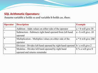
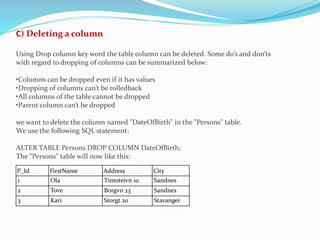
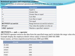
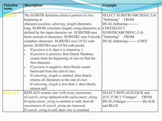
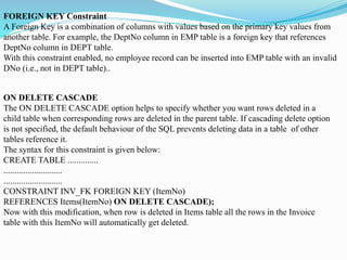
![EMPNO ENAME JOB MGR HIREDATE SAL COMM DEPTNO
7369 SMITH CLERK 7902 12/17/1980 800 - 20
7499 ALLEN SALESMAN 7698 02/20/1981 1600 300 30
7876 ADAMS CLERK 7788 01/12/1983 1100 - 20
7900 JAMES CLERK 7698 12/03/1981 950 - 30
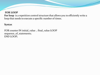
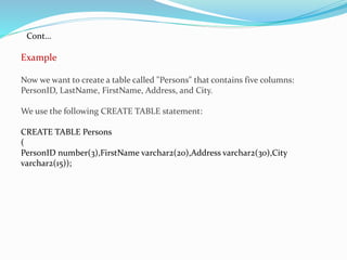
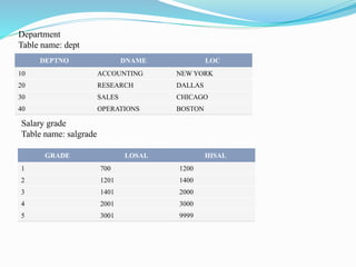
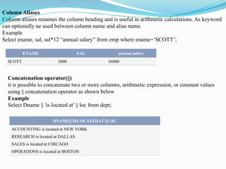
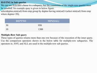
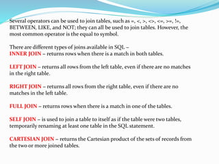
Example 2: logical operator OR
Display employee details whose name starts with A or salary <=1000
Select * from emp where enamelike’A%’ or sal<=1000;
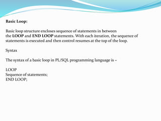
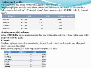
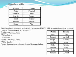
ORDER BY clause (ASC/DESC)
The output of any SQL program is a listing of table data as it is, and no implicit order is used. We
can display data either in ascending or in descending order using the keyword ASC (default) and
DESC respectively. The general syntax is
Select * or Distinct or column name or expression from table name where condition order by
(column name, expression, alias) [ASC/DESC];](https://image.slidesharecdn.com/structurequerylanguagesql-230120062847-a4a43d7b/85/Structure-Query-Language-SQL-pptx-36-320.jpg)
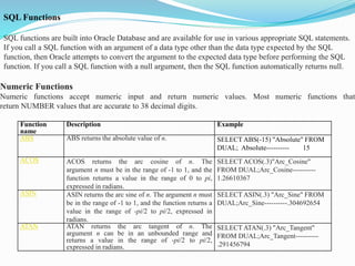
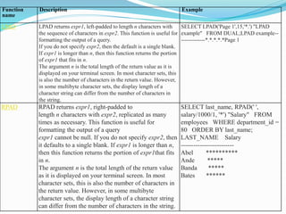
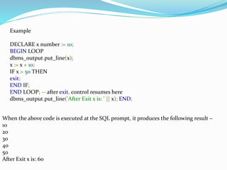
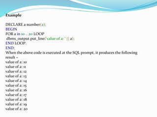
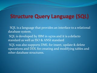
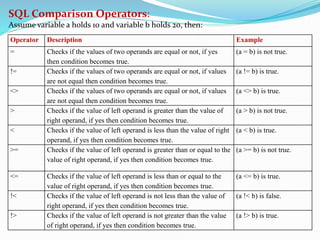
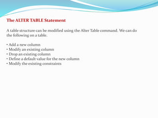
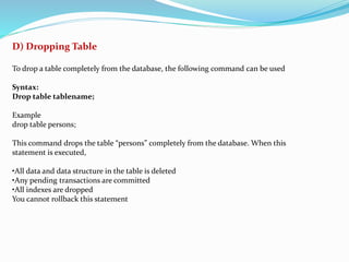
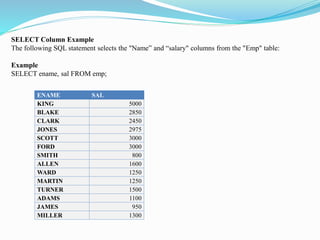
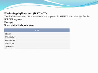
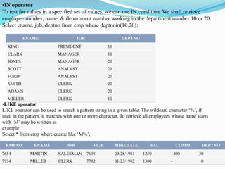
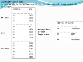
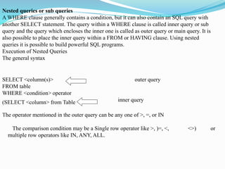
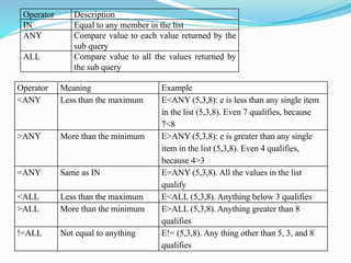
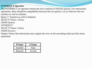
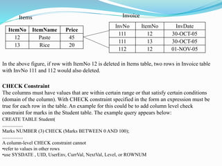
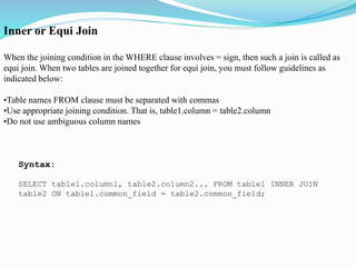
![The general syntax of SELECT Clause with GROUP BY clause is shown below:
SELECT [col, ] group_function(col),
FROM Table
[WHERE condition]
[GROUP BY column]
[HAVING condition]
The rules to be followed while using GROUP BY clause are given below:
•Non-group functions or columns are not allowed in SELECT clause.
•Group Functions ignore nulls.
•By default, the result of GROUP BY clause sorts data in ascending order
Examples
No of Employees
14
Select count(* ) as “No of Employees” from emp;
Select count(job) as " No of Employees" from emp where job='MANAGER';
No of Employees
3](https://image.slidesharecdn.com/structurequerylanguagesql-230120062847-a4a43d7b/85/Structure-Query-Language-SQL-pptx-47-320.jpg)
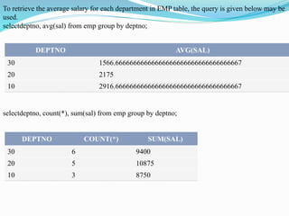
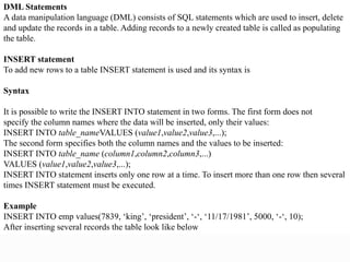
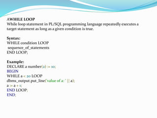
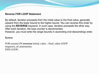
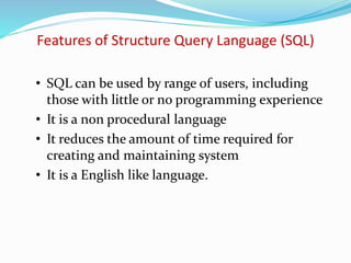
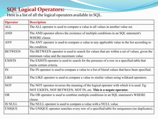
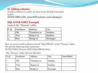
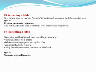
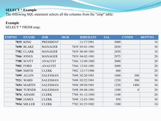
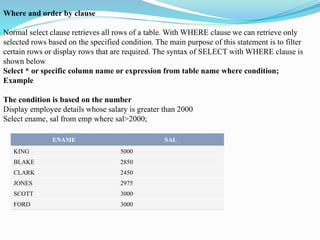
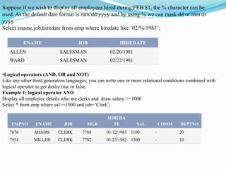
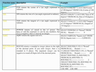
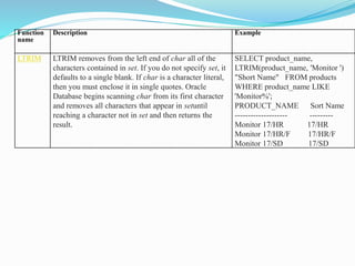
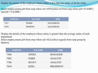
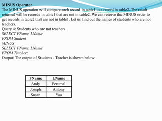
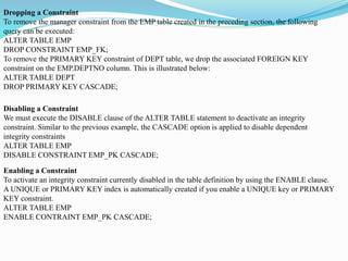
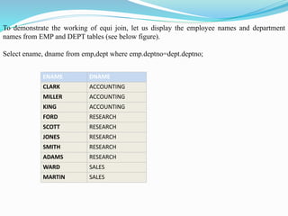
![DELETE Statement
To remove row from a table, use DELETE Statement. The syntax for this statement is given
below
DELETE [FROM] table [WHERE Condition];
The DELETE statement deletes only one row at a time if the WHERE condition contains a
primary key. Be careful that if WHERE is not present in the query, all the rows in the table are
deleted. To delete OPERATIONS department in DEPT table, we use the SQL statement as shown
in below figure
delete from dept where dname='OPERATIONS';
1 row(s) deleted.
An error message may be displayed during a row deletion, if it has a reference in some other
table.
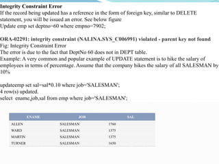
For example, an attempt to delete the row with DeptNo = 10, Oracle SQL displays an integrity
constraint error.
delete from dept where deptno=10;
Error Message: ORA-02292: integrity constraint (SCOTT.SYS_C00810) violated – child record
found
This is because, there are several employees working for department number 10 and these records
appear in EMP table. Hence, unless all these records are deleted, it is not possible to delete the
department](https://image.slidesharecdn.com/structurequerylanguagesql-230120062847-a4a43d7b/85/Structure-Query-Language-SQL-pptx-55-320.jpg)
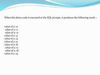
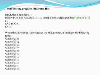
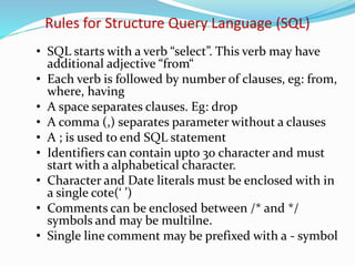
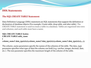
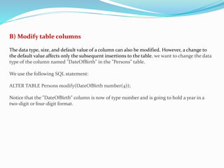
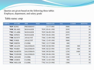
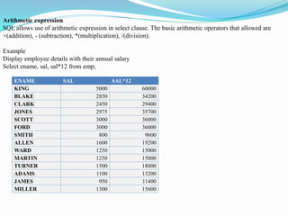
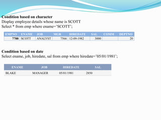
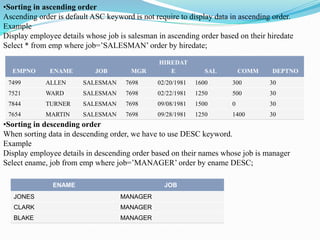
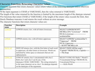
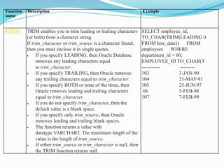
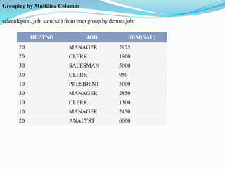
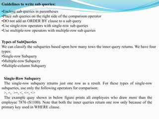
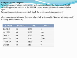
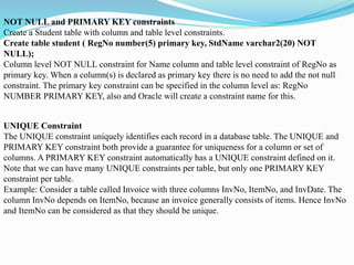
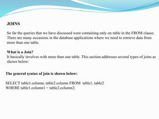
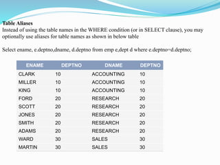
![given below:
UPDATE table
SET column-1 = value-1 [, column-2 = value-2 ………]
[WHERE condition];
UPDATE a Single Row
To update a single row we must use WHERE clause with primary key. Assume that we wish to
promote the employee FORD (EmpNo = 7902) from the job of ANALYST to MANAGER. The
query shown in below figure does this task.
updateemp set job='MANAGER' where empno=7902;
1 row(s) updated.selectempno,ename, job from emp where empno=7902;
EMPNO ENAME JOB
7902 FORD MANAGER](https://image.slidesharecdn.com/structurequerylanguagesql-230120062847-a4a43d7b/85/Structure-Query-Language-SQL-pptx-56-320.jpg)
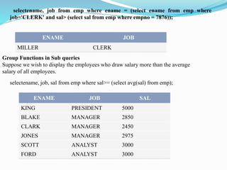
![CONSTRAINTS
Basically constraints enforce certain rules on table or column level. For example, primary key,
foreign key, etc, are some of the table level constraints that can be specified. SQL allows you to
define constraints on columns and tables. Constraints give us as much control over data in tables
as needed. If a user attempts to store data in a column that would violate a constraint, an error is
raised. This applies even if the value came from the default value definition.
Oracle 10g supports the following types of constraints:
NOT NULL
UNIQUE KEY
PRIMARY KEY
FOREIGN KEY
CHECK
Syntax for creating a Constraints
CREATE TABLE [schema.] table (column data type [DEFAULT expr] [column_constraint],
………….[CONSTRAINT constraint_name] constraint_type (column, …..),);
This syntax gives the method to add constraints using the keyword CONSTRAINT. The
column_constraint shown in the second line with bold letters specifies the column level
constraint which takes the same syntax as table level constraint.](https://image.slidesharecdn.com/structurequerylanguagesql-230120062847-a4a43d7b/85/Structure-Query-Language-SQL-pptx-72-320.jpg)
![Constraint Manipulations
The constraints can be added, dropped, enabled, or disabled provided appropriate constraints
have been defined while creating the table. A constraint cant’t be modified directly, but follow
a two step process. First, drop the existing constraint, and then add a new constraint with
intended modifications.
Adding a Constraint
To add a constraint, use the following syntax:
ALTER TABLE table_name
ADD [CONSTRAINT constraint] type (column);
Look at the below example,
ALTER TABLE EMP
ADD CONSTRIANT EMP_FK
FOREIGN KEY(Mgr) REFERENCES EMP(EmpNo);
This example adds a foreign key constraint to EMP table, but in general you can add any type
of constraint.](https://image.slidesharecdn.com/structurequerylanguagesql-230120062847-a4a43d7b/85/Structure-Query-Language-SQL-pptx-76-320.jpg)
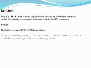
![Cross Join:
The CARTESIAN JOIN or CROSS JOIN returns the Cartesian product of the sets of
records from two or more joined tables. Thus, it equates to an inner join where the
join-condition always evaluates to either True or where the join-condition is absent
from the statement.
Syntax:
The basic syntax of the CARTESIAN JOIN or the CROSS JOIN is as follows −
SELECT table1.column1, table2.column2... FROM table1,
table2 [, table3 ]](https://image.slidesharecdn.com/structurequerylanguagesql-230120062847-a4a43d7b/85/Structure-Query-Language-SQL-pptx-92-320.jpg)
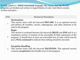
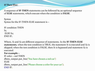
![Variable Declaration in PL/SQL
PL/SQL variables must be declared in the declaration section or in a package as a
global variable. When you declare a variable, PL/SQL allocates memory for the
variable's value and the storage location is identified by the variable name.
The syntax for declaring a variable is −
variable_name [CONSTANT] datatype [NOT NULL] [:= | DEFAULT initial_value]
Where, variable_name is a valid identifier in PL/SQL, datatype must be a valid
PL/SQL data type. Some valid variable declarations along with their definition
are shown below −
sales number(10, 2);
pi CONSTANT double precision := 3.1415;
name varchar2(25);
address varchar2(100);](https://image.slidesharecdn.com/structurequerylanguagesql-230120062847-a4a43d7b/85/Structure-Query-Language-SQL-pptx-100-320.jpg)