Download to read offline
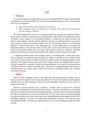
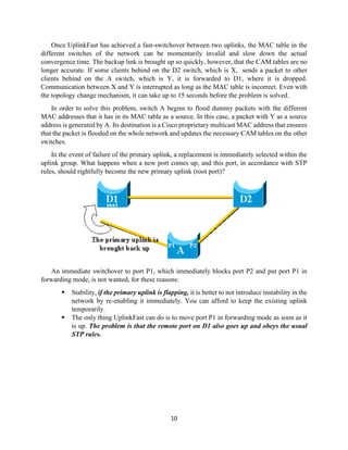
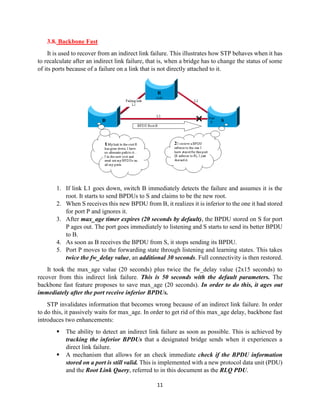
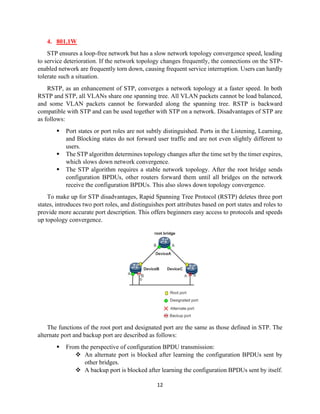
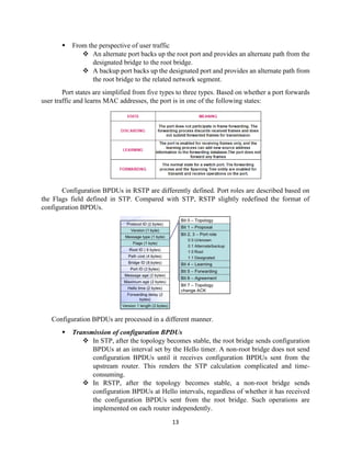


The document details the Spanning Tree Protocol (STP), which prevents broadcast storms by managing redundant paths in networks. It explains how STP operates using bridges, with mechanisms for determining which paths to include in the active forwarding topology, and introduces various enhancements like PortFast, BPDU guard, and UplinkFast to improve network stability and reduce recovery times from failures. The document highlights the continuous, distributed process of maintaining a loop-free network topology while addressing potential issues with path changes and link failures.