Download to read offline
![7
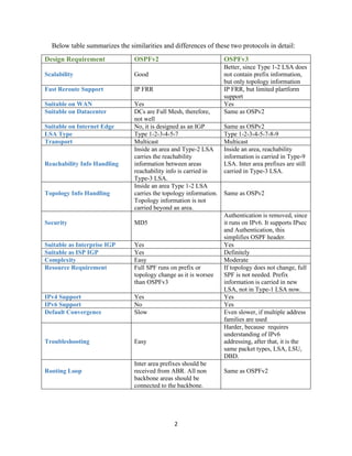
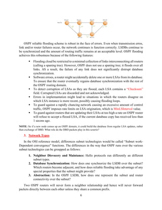
3.1.Broadcast
Data link whereby on attached node can send a single paclet that will be received by all other
nodes attached the subnet. Broadcast is very useful for autoconfiguration and replicating
information.
Now let's perform our examination in the following items over 3 main topics on the previous
page:
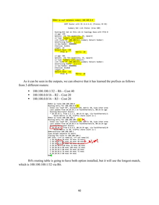
1. Each OSPF routers periodically multicasts its Hello packets to the IP address 224.0.0.5
or 224.0.0.6. The advantages of over broadcast subnets are floows:
❖ Automatic discovery of neighbors
❖ Efficiency when N router are on a broadcast segment, there are [N(N-1)]/2
neighbor relationship and are maintened by sending only N Hello packets.
❖ Isolation
2. On a broadcast subnet with N routers, there are [N(N-1)]/2 neighbor pairs. If you try to
synchronize databases between every pair of routers, you end up with a large number
of LSU and LSAck being sent over the subnet. Therefore, OSPF solves this problem
by electing a DR, BDR for the broadcast subnet. Using the normal procedures of the
database exchange and reliable flooding.
3. The obvious way to do this is for each router to include links to all other routers in its
“Router LSA”. But this would introduce N(N-1) links into the OSPF database, so
instead OSPF creates a new LSA type, which is called “Network LSA”.
3.2.Point to Point
A network that joins a single pair of routers. Here’s what you need to know about OSPF point-
to-point:
▪ Automatic neighbor discovery so no need to configure OSPF neighbors yourself.
▪ No DR/BDR election since OSPF sees the network as a collection of P2P links.
▪ Normally uses for point-to-point sub-interfaces with an IP subnet per link.
▪ Can also be used with multiple PVCs using only one subnet.](https://image.slidesharecdn.com/ospf-200428102847/85/Open-Shortest-Path-First-7-320.jpg)
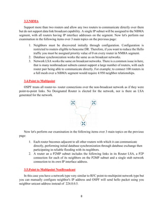
![18
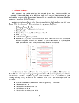
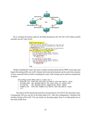
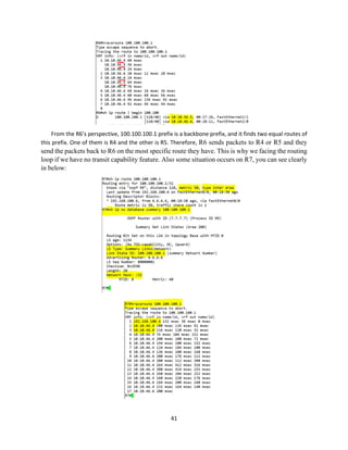
▪ Intra-Area [O]: Routes originated within an area, are known by the routers in the same
area as Intra-Area routes. These routes are flagged as O. Also called OSPF Internal
routes, as they are generated by OSPF itself, when an interface is covered with the
OSPF network command.
▪ Inter-Area [O IA]: When a route crosses an ABR, the route is known as an OSPF
Inter-Area route. These routes are flagged as O IA. Also called OSPF Internal routes,
as they are generated by OSPF itself, when an interface is covered with the OSPF
network command.
▪ NSSA Type 1 [N1]: When an area is configured as a NSSA, and routes are redistributed
into OSPF, the routes are known as NSSA External Type-1. These routes are flagged
as O N1.
▪ External Type 1 [E1]: Routes which were redistributed into OSPF, such as connected,
static, or other routing protocol, are known External Type-1. These routes are flagged
as O E1. A cost is the addition of the external cost and the internal cost used to reach
that route.
▪ NSSA Type 2 [N2]: The definition for type O N1 is valid for this route type. Also,
these routes are flagged as O N2.
▪ External Type 2 [E2]: The definition for type E1 is valid for this route type, with one
difference, which is the cost is always the external cost, irrespective of the interior cost
to reach that route. Also, these routes are flagged as O E2.
There is a common question in here, which is better E1 or E2 routes? This preference comes
from the root belief that OSPF as a routing protocol, which is uses cost as it metric, shoul never
disregard cost from making routing decisions. Therefore, E1 routes are preferred by many because
they take into account the cost of the links to the external network ehenever you are in the OSPF
AS. Consider using E1 routes under the following circumstances:
▪ Your network has multiple exit points, from your OSPF AS to the same external AS
▪ Your network has multiple paths to a single external network from mant destinations
Some defining characteristics and needs of E2 routes are as folow:
▪ The default route generated by a stub Abr is on E2 route into the stub are because a
stub network is usually simple in its topology. So, there is just one way out!!
▪ Your ntwork is not very large, and thus you do not need E1 routes](https://image.slidesharecdn.com/ospf-200428102847/85/Open-Shortest-Path-First-18-320.jpg)
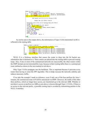
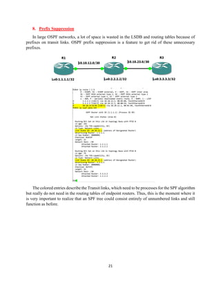
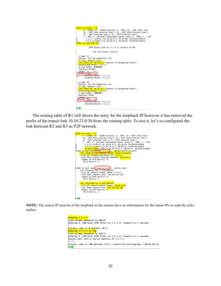
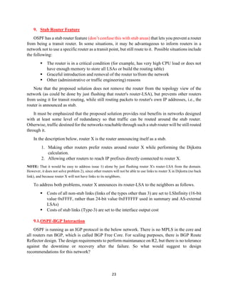

OSPF is a link-state routing protocol that uses link-state information to make routing decisions. Each router running OSPF floods link-state advertisements (LSAs) throughout the area or autonomous system that contain information about that router's attached interfaces and metrics. Routers then use the information in LSAs to calculate the shortest path to each network and build routing tables. OSPF supports different network types including broadcast, point-to-point, non-broadcast multi-access (NBMA), and point-to-multipoint. It elects a designated router on broadcast networks to reduce the number of adjacencies formed and amount of routing information exchanged.