Pti systems

1. Analysis of LTI Systems using
Difference Equations
Dr. Pooja Sahni

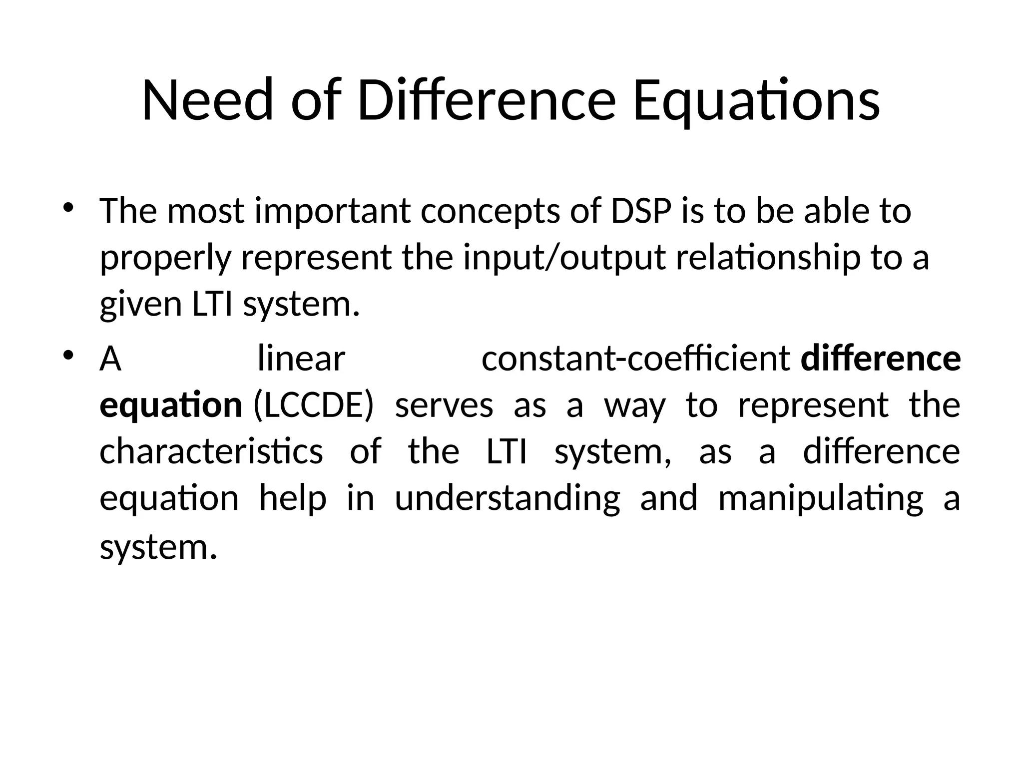
2. Need of Difference Equations
• The most important concepts of DSP is to be able to
properly represent the input/output relationship to a
given LTI system.
• A linear constant-coefficient difference
equation (LCCDE) serves as a way to represent the
characteristics of the LTI system, as a difference
equation help in understanding and manipulating a
system.

3. Difference Equation
• Definition
An equation that shows the relationship between
consecutive values of a sequence and the differences
among them. They are often rearranged as a
recursive formula so that a systems output can be
computed from the input signal and past outputs.
Example : y[n]+7y[n−1]+2y[n−2]=x[n]
−4x[n−1]

4. A discrete time system takes discrete time input signal
{ x[ n ] },& produces an output signal { y[ n ] }.
•Implemented by general purpose computer,
microcomputer or dedicated digital hardware capable
of carrying out arithmetic operations on samples of
{x[n]} and {y[n]}.
SYSTEM
input
{x[n]}
output
{y[n]}
Concepts

5. • {x[n]} is sequence whose value at t=nT is x[n]. T is sampling
interval in seconds.
• 1/T is sampling frequency in Hz.
• {x[n-N]} is sequence whose value at t=nT is x[n-N].
{x[n-N]} is {x[n]} with every sample delayed
by N sampling intervals.
(i) Discrete time "amplifier" with output: y[n] depending on
present input only
y[n] = A . x[n]. Described by“ difference equation"
• Represented in diagram form by a "signal flow graph” .
x[n] y[n]
A

6. (ii) Processing system whose output at t=nT is obtained by
weighting & summing present & previous input samples:
y[n] = A0 x[n] + A1 x[n-1] + A2 x[n-2] + A3 x[n-3] + A4x[n-4]
‘Non-recursive difference equatn’ with signal flow graph below.
Boxes marked " z-1
" produce a delay of one sampling interval.
z-1
z-1
z-1 z-1
x[n]
A0 A1
A2 A3 A4
y[n]

7. (iii) System whose output y[n] at t = nT is calculated according to
the following recursive difference equation:
y[n] = A0 x[n] - B1 y[n-1]
whose signal flow graph is given below.
• Recursive means that previous values of y[n] as well as
present & previous values of x[n] are used to calculate y[n].
z-1
x[n] A0
B1
y[n]

8. (iv) A system whose output at t=nT is:
y[n] = (x[n])2
as represented below.
x[n] y[n]

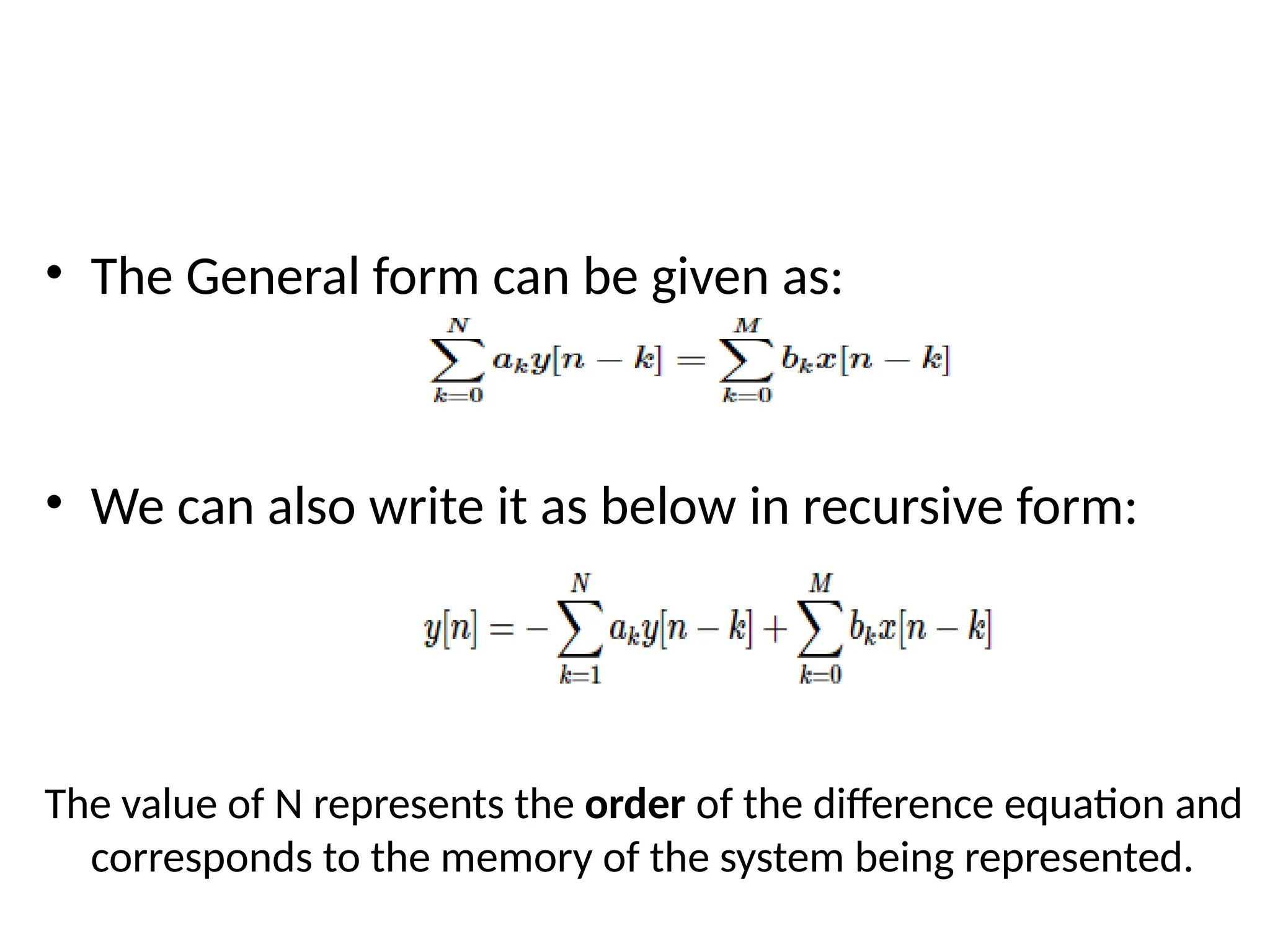
9. • The General form can be given as:
• We can also write it as below in recursive form:
The value of N represents the order of the difference equation and
corresponds to the memory of the system being represented.

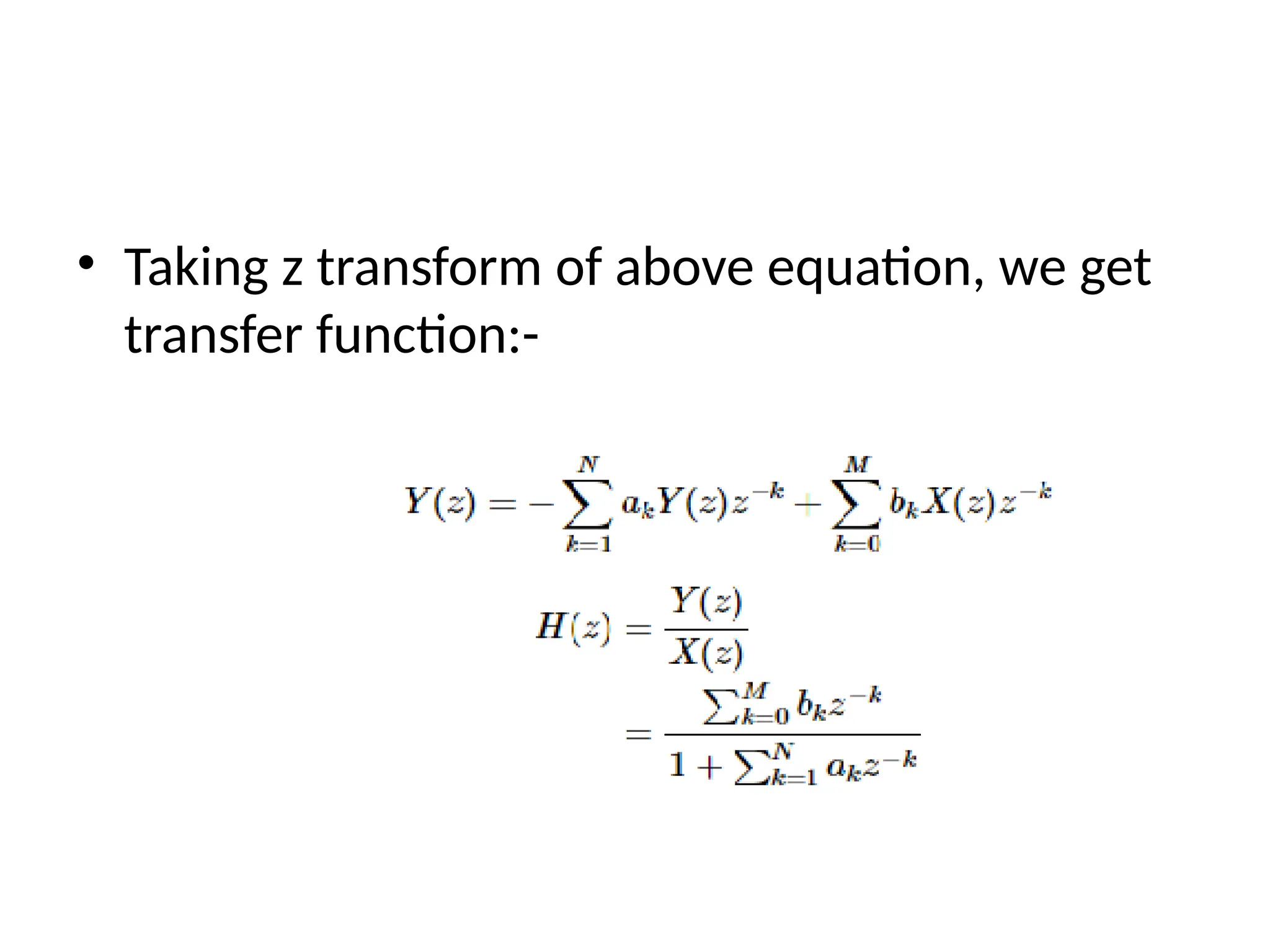
10. • Taking z transform of above equation, we get
transfer function:-

11. Solving a LCCDE
• Two common methods exist for solving a
LCCDE:
• The direct method
• The indirect method

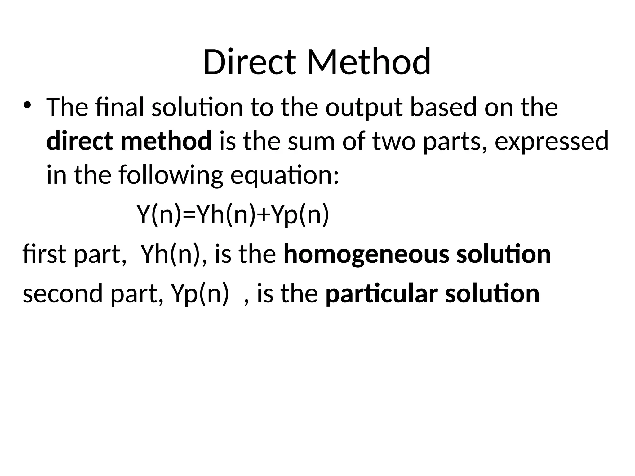
12. Direct Method
• The final solution to the output based on the
direct method is the sum of two parts, expressed
in the following equation:
Y(n)=Yh(n)+Yp(n)
first part, Yh(n), is the homogeneous solution
second part, Yp(n) , is the particular solution

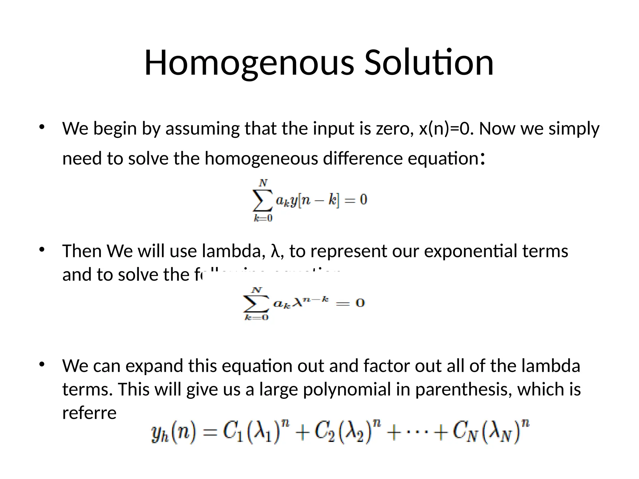
13. Homogenous Solution
• We begin by assuming that the input is zero, x(n)=0. Now we simply
need to solve the homogeneous difference equation:
• Then We will use lambda, λ, to represent our exponential terms
and to solve the following equation:
• We can expand this equation out and factor out all of the lambda
terms. This will give us a large polynomial in parenthesis, which is
referred to as the characteristic polynomial

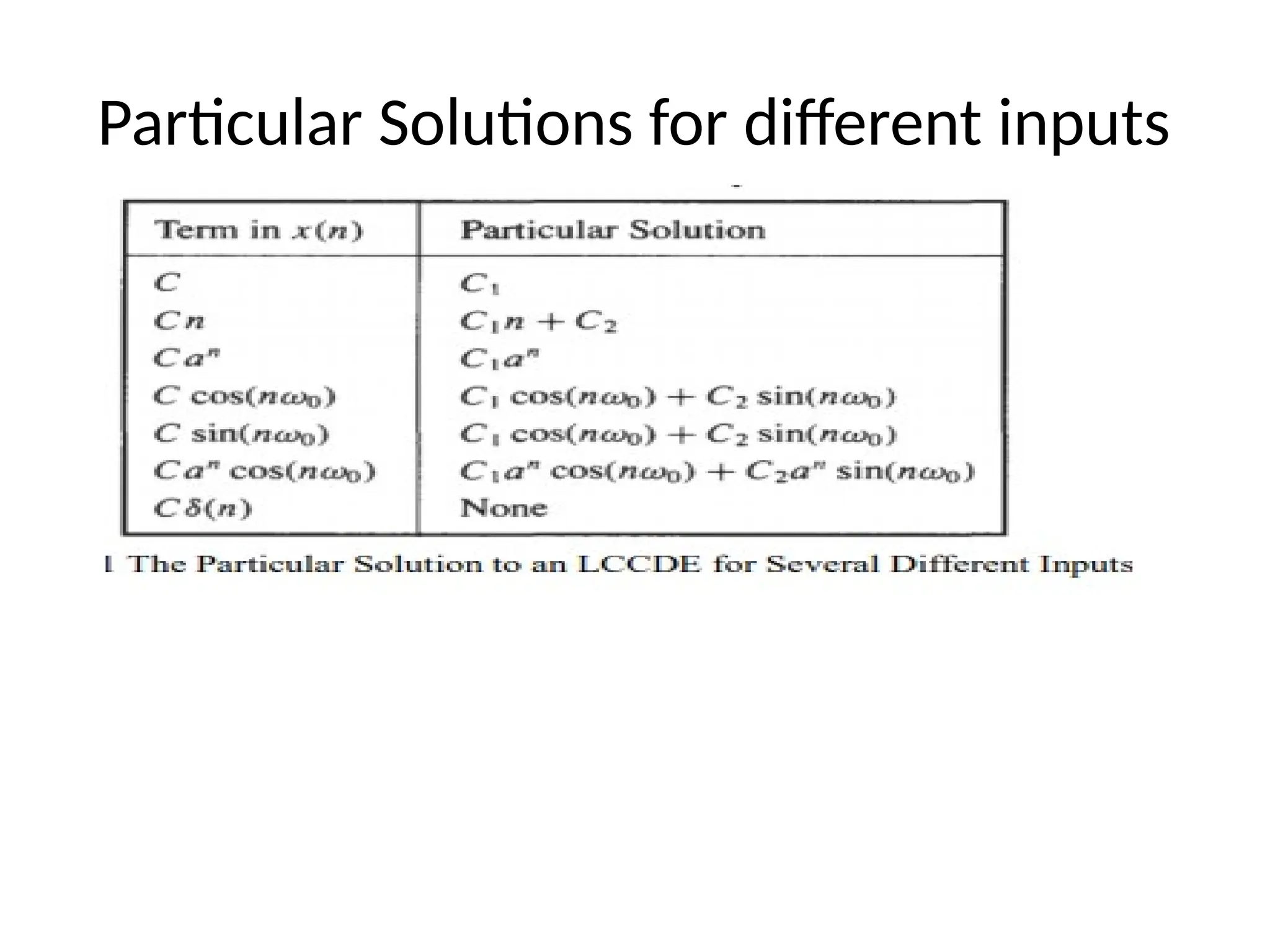
14. Particular Solution
• The particular solution, Yp(n), will be any solution that will solve
the general difference equation:
• Then the particular solution will be in form:
• for x(n) = Cδ(n) the particular solution is zero.
Because x(n) = 0 for n > 0

15. Particular Solutions for different inputs

16. Examples