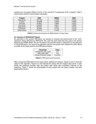
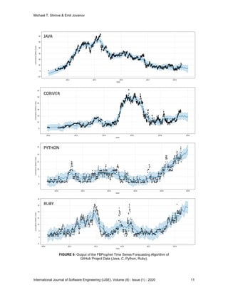
The research provides a framework for forecasting software defect trends in open-source projects using univariate ARIMA and FBProphet models. It emphasizes the importance of real-time forecasting to allocate resources effectively and reduce software failures, showcasing results from analyzing seven projects over time. The study concludes that these models can predict defects up to six months in advance with a low mean square error, enhancing project management strategies.
![Michael T. Shrove & Emil Jovanov
International Journal of Software Engineering (IJSE), Volume (8) : Issue (1) : 2020 1
Software Defect Trend Forecasting In Open Source Projects
using A Univariate ARIMA Model and FBProphet
Michael T. Shrove tshrove@gmail.com
Millennium Corporation
Huntsville, AL. 35806, USA
Emil Jovanov emil.jovanov@uah.edu
ECE Department
University of Alabama Huntsville
Huntsville, AL. 35899, USA
Abstract
Our objective in this research is to provide a framework that will allow project managers, business
owners, and developers an effective way to forecast the trend in software defects within a
software project in real-time. By providing these stakeholders with a mechanism for forecasting
defects, they can then provide the necessary resources at the right time in order to remove these
defects before they become too much ultimately leading to software failure. In our research, we
will not only show general trends in several open-source projects but also show trends in daily,
monthly, and yearly activity. Our research shows that we can use this forecasting method up to 6
months out with only an MSE of 0.019. In this paper, we present our technique and
methodologies for developing the inputs for the proposed model and the results of testing on
seven open source projects. Further, we discuss the prediction models, the performance, and the
implementation using the FBProphet framework and the ARIMA model.
Keywords: Software Engineering, Software Defects, Time Series Forecasting, ARIMA,
FBProphet.
1. INTRODUCTION
In today’s world, software has almost become a part of every job function in the market. From the
food industry to the medical industry to the defense industry, software is everywhere. Which in
turn, means more and more people rely on software that is of high quality and produces accurate
results. However, in 2015 a report by Standish Group showed that only 29% of software projects
are successful and 52% were “challenged”[1]. Even in the 52% that were “challenged”, do we
know they produced a quality product? A successful project does not necessarily mean, a quality
product.
In [2], the authors lay out four main high-level areas for why software projects fail, People, Tasks,
Environment, Methods. In this study, one of the main areas that we focused on was the lack of
software testing, which directing was related to software project failure. In turn, the lack of
software testing can lead to more software defects which inevitably leads to software failure.
In this research, we propose a time series model for forecasting trends and patterns in software
project defect data in order for stakeholders to reallocated resources. In our proposed solution,
we show that unlike most research in this area, our approach can be performed in real-time using
a new framework called FBProphet and show much more than just the trend in overall defect
data. We also show that we can present daily, weekly, and yearly seasonal trends. This trend
analysis can be used to effectively show where to reallocate resources up to weeks and months
in the future on the project. If stakeholders can know what their defect posture will look like in the
future, it may give software project’s a higher probability of success. In the section label, Review
of Literature, we will be reviewing papers and related research to this area. In the Overall](https://image.slidesharecdn.com/ijse-167-200925053606/85/Software-Defect-Trend-Forecasting-In-Open-Source-Projects-using-A-Univariate-ARIMA-Model-and-FBProphet-1-320.jpg)
![Michael T. Shrove & Emil Jovanov
International Journal of Software Engineering (IJSE), Volume (8) : Issue (1) : 2020 2
Approach section, we present the overall approach, data used in our research, and the models
used to forecast trends and patterns. After that, we show the results of our research in the
Results section. Lastly, in Threat to Validity, we present threats to the validity of our research and
present some mitigations against it.
2. REVIEW OF LITERATURE
In performing literature reviews for similar research, what we found was that a majority of authors
focusing in this area, more specifically with defect counts, are trying to classify if a particular code
module is or will be defect prone based on software metrics [3][4][5][6][7][8][9]. In our research,
we are focused on the more project management aspects of the project. Forecasting trends,
similar to financial market trends [10], in the total defect counts, to use for decision making
[11][12].
Our research builds on top of Raja and Hale’s research in [13]. Raja et al. showed an auspicious
method in using defects to get accurate trend analysis from technical debt items from a software
project. We followed their research and laid out the same approach as them. However, in our
research, we wanted to make it more practical and more user-friendly for the practitioner. With
the increase in data generating in these software projects, so has the need and popularity in
using machine learning and statistical-based models to be able to make sense of these data
while not adding burden to the practitioner. In [14], Manzano et al. presented an API-based
framework for using statistical models in a more manageable approach by proposing these
models to be behind an API but still using ARIMA as the model, which is the same statistical
method in research.
In [16], Chikkakrishna et al. showed a more user-friendly method by using the FBProphet
framework to get seasonal trends from the data more efficiently than from the ARIMA-based
model. Chikkakrishna et al. used both an ARIMA method along with FBProphet to supplement
getting more information from the data as we did in our research.
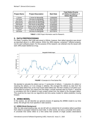
3. OVERALL APPROACH
In our approach, we wanted to find a method that would allow software project stakeholders to
monitor the data, present the total number of defects, forecast the trends in the data, and present
in a graphic format for the stakeholders to view for decision making. For the data, we focused on
open source software (OSS) project data, with no use of simulation. We needed to find some that
had their defect data open to the public. We used OSS to apply time series-based models to
forecast trends in the data, and lastly, we used open-source graphing libraries to present the
trends to the stakeholders.
4. THE TRAINING DATASET
Our training datasets is open-source software projects from a company called MongoDB. They
were readily available and open to the public and was acquired using MongoDB’s JIRA API.
MongoDB has been tracking a set of their software projects over the past 9 years using Atlassian
JIRA as their issue tracking system. Their projects are mostly the drivers used for connecting
various programming languages to the MongoDB platform. There was a total of 31 projects in
their JIRA instance. Out of the 31 projects, we chose 7 for our research. Out of the 7 projects, the
mean lifespan was 9.64 years ± 172 days. The shortest project currently has a lifespan of 3,286
days and the longest project having a lifespan of 3,679 days, as seen in Table 1.
In [15] the authors showed that there is a very clear correlation between testing and software
defects. Moreover, OSS does not typically have dedicated testers, testing strategies, and test
procedures in place to find defects consistently. Therefore, we chose MongoDB’s projects
because the projects themselves were made available to the public, however, the projects were
backed by a public company with development processes and testing.](https://image.slidesharecdn.com/ijse-167-200925053606/85/Software-Defect-Trend-Forecasting-In-Open-Source-Projects-using-A-Univariate-ARIMA-Model-and-FBProphet-2-320.jpg)
![Michael T. Shrove & Emil Jovanov
International Journal of Software Engineering (IJSE), Volume (8) : Issue (1) : 2020 4
recorded sequentially over equal time increments [17]. There are many different techniques and
methods for time series forecasting which include: autoregressive moving average (ARMA),
autoregressive integrated moving average (ARIMA), Exponential Smoothing, and Holt-Winters. In
this research, we will be focusing on using the ARIMA model or sometimes referred to as the Box
Jenkins Model. The ARIMA model is a combination of both the autoregressive (AR) models and
the moving average (MA) models.
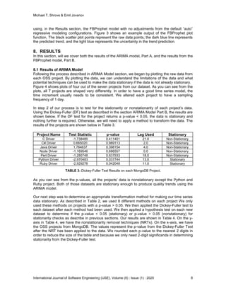
6.2 Stationality Testing
One assumption about using the ARIMA model is that the data is required to be stationary.
Stationary is defined as the mean, variance and autocovariance do not change over time. Later in
our research, we will show our techniques for removing nonstationarity, the most common
technique being differencing. In our research, in order to determine if our time series was
stationary or not, we used the Dickey-Fuller (DF) test [18].The DF test suggests the time series
has a unit root, meaning it is nonstationary. It has some time-dependent structure. The alternative
hypothesis is that it suggests the time series does not have a unit root, meaning it is stationary. It
does not have a time-dependent structure. Once the DF test has been run, if the time series was
stationary (p-value < alpha value) we could move on to applying the ARIMA model, if not, we
would have to apply methods for removing nonstationarity in the data.
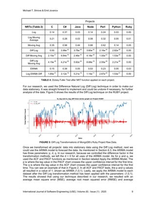
6.3 Methods for Removing Nonstationality
Methods for removing nonstationarity are not the same each time for time series data. Different
methods must be applied each time, and the results must be manually evaluated based on the
results of the hypothesis test. The most common techniques for removing nonstationarity are
transformation, smoothing, and differencing. Of those 3 techniques, we used 8 methods shown in
Table 2.
# Name Technique Description
1 Natural Log Transformation Applying the natural logarithm to the data.
2 Log Moving Average
Transformation /
Smoothing
Applying a 7-day moving average of the
natural logarithm of the data.
3 Moving Average Smoothing
Applying a 7-day moving average of the
data.
4 Diff Natural Log
Transformation /
Differencing
Applying differencing to the natural
logarithm of the data.
5 Diff Moving Average and Data Transformation
Applying the difference between normal
data and moving average.
6 Diff Log and Moving Average
Transformation
/Differencing
Applying a difference between the natural
logarithm of the data and the natural
logarithm moving average.
7
EWMA (Exponential Weighted
Moving Average) of Log
Transformation
Applying an EWMA algorithm to the
natural logarithm of the data. We used a
half-life of 7 for all instances.
8 Log EWMA Differencing
Transformation /
Differencing
Applying a difference between the natural
logarithm of the data with the EWMA
algorithm.
TABLE 2: Non-Stationarity Removal Techniques (NRTs).](https://image.slidesharecdn.com/ijse-167-200925053606/85/Software-Defect-Trend-Forecasting-In-Open-Source-Projects-using-A-Univariate-ARIMA-Model-and-FBProphet-4-320.jpg)
![Michael T. Shrove & Emil Jovanov
International Journal of Software Engineering (IJSE), Volume (8) : Issue (1) : 2020 5
In each of our hypothesis tests (applying the DF test to each technique), we used a value of 0.05.
If the results of the hypothesis test returned a value less than 0.05, we would fail to reject the null
hypothesis (not stationary). Otherwise, if the p-value was equal to or greater than 0.05, we would
reject the null hypothesis and we could potentially use the technique for removing the
nonstationarity in the data.
6.4 Applying The ARIMA Model
In an ARIMA model as defined in earlier texts are three parts of the equation, autoregressive
(AR), integrated (I) and moving average (MA). Lags of the stationarized series in the forecasting
equation are the AR, lags of the forecast errors are the MA, and a time series which needs to be
differenced to be made stationary is said to be an "integrated (I)" version of a stationary series
[19]. Often times the ARIMA model will be shown as ARIMA (P,D,Q) where P refers to
the number of AR terms, D refers to the number of nonseasonal differences needed for
stationarity, and Q refers to the number of lagged forecast errors in the prediction equation.
In our research in order to determine the P and Q parameters in the ARIMA model, we used the
Partial Autocorrelation Function (PACF) and the Autocorrelation Function (ACF) respectively. The
ACF is the correlation between the time series and the lagged version of itself. The PACF is
explained as an additional correlation explained by each successive lagged term. Figure 2 shows
an example of the ACF and PACF functions. Lastly, we apply the ARIMA model to the data. We
use the chosen data based on the hypothesis tests from removing nonstationarity and using the
parameters shown to the correct parameters for P, D, and Q using the ACF and PACF functions.
During our results, we used more than one nonstationarity method. Our results of the ARIMA
model will be shown in the Results section.
FIGURE 2: Example of ACF and PACF Outputs.](https://image.slidesharecdn.com/ijse-167-200925053606/85/Software-Defect-Trend-Forecasting-In-Open-Source-Projects-using-A-Univariate-ARIMA-Model-and-FBProphet-5-320.jpg)
![Michael T. Shrove & Emil Jovanov
International Journal of Software Engineering (IJSE), Volume (8) : Issue (1) : 2020 6
7. FBProphet
Prophet is an open-source forecasting tool developed by Facebook’s core data science team. It is
used for forecasting time series data based on an additive model where non-linear trends are fit
with yearly, weekly, and daily seasonality, plus holiday effects. It works best with time series that
have strong seasonal effects and several seasons of historical data [20]. With FBProphet you
can either “auto” forecast or customize it using some of the configurations built-in [21].
Underneath it all, FBProphet uses ARIMA, exponential models, and other similar regressive
models. We will be
FIGURE 3: Example out of a FBProphet plot using the Mongo
Python Project Data](https://image.slidesharecdn.com/ijse-167-200925053606/85/Software-Defect-Trend-Forecasting-In-Open-Source-Projects-using-A-Univariate-ARIMA-Model-and-FBProphet-6-320.jpg)
![Michael T. Shrove & Emil Jovanov
International Journal of Software Engineering (IJSE), Volume (8) : Issue (1) : 2020 13
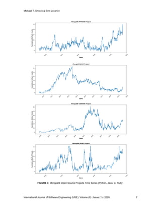
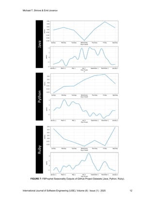
As you can see from the seasonalities, specifically the weekly, three projects (JAVA and RUBY)
seem to have a trend of decreasing the defects from Sunday to Wednesday then producing
defects from Wednesday to Saturday. The Python project seem to produce defects during the
week and fix them over the weekend and lastly. Similarly, you can see other trends in the data
through the yearly trends.
9. THREATS TO VALIDITY
In this section, will we cover what in the research by be a threat to producing valid research.
9.1 Data Validity
The defects collected in our data are defects reported by people in the open-source community.
These people may be amateurs to the product, or they could be internal MongoDB personnel. We
don’t really have any knowing, therefore, the reported defects may not be valid or there may be
duplicates of the same defect.
9.2 Variation of Data
The data collected during this research was all collected from one source, MongoDB. Having
different sources of data could show a broader trend in seasonality and defect reporting that is
not shown in the data. Future research will collect multiple sources and perform a similar analysis
and come to a more general and common model for the general software community.
9.3 Reporting Mechanisms
The data collected for this research was gathered on MongoDB’s JIRA repository, however,
MongoDB could have another internal reporting instance of JIRA not displayed to the public. This
would not reflect in our data or model development. In future research, we could reach to
MongoDB to confirm one instance of JIRA for defect reporting.
10.FUTURE RESEARCH
The overall goal of our research is to predict the outcome of software projects (success or failure)
using the method described in this research, along with other metrics. To identify whether a
software project is successful or unsuccessful, we need to define what success is. Traditional
waterfall approaches have a defined success and failure defined with cost, schedule, and
performance. However, agile and open-source projects do not necessarily have a defined
success. The one thing that defines success for open source projects is the use of the source of
the number of active users. For agile projects, we plan to use defect trend analysis, presented
here, along with other metrics such as # of pull requests, # active users, # followers for a GitHub
project. We then take those two inputs and define an algorithm to produce a metric that defines a
metric such as the sP2D2 metric presented in [22]. We then can use that to show a real-time
evaluation of whether an agile/open-source project is currently successful based on users and
defects.
11.CONCLUSION
By providing a trend mechanism as seen by FBProphet and the ARIMA model in our research,
these mechanisms could provide valuable insight for the stakeholders of the projects or even the
open-source community. By knowing when defects tend to arrive throughout the week and year,
the stakeholders could easily provide campaigns with the open-source community to ask for
additional help or for-profit companies could plan part-time or temporary resources throughout the
year to reduce the defects without paying for full-time employees. Saving the company money in
the long run. In this research, we have shown that using either the FBProphet or ARIMA models
along with transformation functions, one can forecast defect trends with confidence. We have
also shown that using the FBProphet model can reduce “time-to-market” on producing a model
but may not produce as accurate results as the ARIMA model. In future research, we plan to pair
this research (defect forecasting) with other machine learning models such as classifiers to
potential classify OSS projects as failing projects.](https://image.slidesharecdn.com/ijse-167-200925053606/85/Software-Defect-Trend-Forecasting-In-Open-Source-Projects-using-A-Univariate-ARIMA-Model-and-FBProphet-13-320.jpg)
![Michael T. Shrove & Emil Jovanov
International Journal of Software Engineering (IJSE), Volume (8) : Issue (1) : 2020 14
12. REFERENCES
[1] S. Wojewoda and S. Hastie, “Standish Group 2015 Chaos Report - Q&A with Jennifer
Lynch,” 2015. [Online]. Available: https://www.infoq.com/articles/standish-chaos-2015/.
[Accessed: 25-Aug-2019].
[2] Lehtinen, T., Mäntylä, M., Vanhanen, J., Itkonen, J., & Lassenius, C. (2014). Perceived
causes of software project failures – An analysis of their relationships. Information and
Software Technology, 56(6), 623–643. https://doi.org/10.1016/j.infsof.2014.01.015
[3] Fenton, N., Neil, M., Marsh, W., Hearty, P., Marquez, D., Krause, P., & Mishra, R. (2007).
Predicting software defects in varying development lifecycles using Bayesian nets.
Information and Software Technology, 49(1), 32–43.
https://doi.org/10.1016/j.infsof.2006.09.001
[4] Lessmann, S., Baesens, B., Mues, C., & Pietsch, S. (2008). Benchmarking Classification
Models for Software Defect Prediction: A Proposed Framework and Novel Findings. IEEE
Transactions on Software Engineering, 34(4), 485–496. https://doi.org/10.1109/TSE.2008.35
[5] Okutan, A., & Yıldız, O. (2014). Software defect prediction using Bayesian networks.
Empirical Software Engineering, 19(1), 154–181. https://doi.org/10.1007/s10664-012-9218-8
[6] Qinbao Song, Zihan Jia, Shepperd, M., Shi Ying, & Jin Liu. (2011). A General Software
Defect-Proneness Prediction Framework. IEEE Transactions on Software Engineering,
37(3), 356–370. https://doi.org/10.1109/TSE.2010.90
[7] V. Vashisht, M. Lal, and G. S. Sureshchandar, “A Framework for Software Defect Prediction
Using Neural Networks,” J. Softw. Eng. Appl., vol. 08, no. 08, pp. 384–394, 2015.
[8] Shuo Wang, & Xin Yao. (2013). Using Class Imbalance Learning for Software Defect
Prediction. IEEE Transactions on Reliability, 62(2), 434–443.
https://doi.org/10.1109/TR.2013.2259203
[9] Nam, J., Fu, W., Kim, S., Menzies, T., & Tan, L. (2018). Heterogeneous Defect Prediction.
IEEE Transactions on Software Engineering, 44(9), 874–896.
https://doi.org/10.1109/TSE.2017.2720603
[10] Bou-Hamad, I., & Jamali, I. (2020). Forecasting financial time-series using data mining
models: A simulation study. Research in International Business and Finance, 51.
https://doi.org/10.1016/j.ribaf.2019.101072
[11] Weber, R., Waller, M., Verner, J., & Evanco, W. (2003). Predicting software development
project outcomes. Lecture Notes in Computer Science (including Subseries Lecture Notes in
Artificial Intelligence and Lecture Notes in Bioinformatics), 2689, 595–609.
https://doi.org/10.1007/3-540-45006-8_45
[12] Ramaswamy, V., Suma, V., & Pushphavathi, T. (2012). An approach to predict software
project success by cascading clustering and classification. IET Seminar Digest, 2012(4).
https://doi.org/10.1049/ic.2012.0137
[13] Raja, U., Hale, D., & Hale, J. (2009). Modeling software evolution defects: a time series
approach. Journal Of Software Maintenance And Evolution-Research And Practice, 21(1),
49–71. https://doi.org/10.1002/smr.398
[14] Manzano, M., Ayala, C., Gomez, C., & Lopez Cuesta, L. (2019). A Software Service
Supporting Software Quality Forecasting. 2019 IEEE 19th International Conference on
Software Quality, Reliability and Security Companion (QRS-C), 130–132.
https://doi.org/10.1109/QRS-C.2019.00037](https://image.slidesharecdn.com/ijse-167-200925053606/85/Software-Defect-Trend-Forecasting-In-Open-Source-Projects-using-A-Univariate-ARIMA-Model-and-FBProphet-14-320.jpg)
![Michael T. Shrove & Emil Jovanov
International Journal of Software Engineering (IJSE), Volume (8) : Issue (1) : 2020 15
[15] Fenton, N., & Neil, M. (1999). A critique of software defect prediction models. IEEE
Transactions on Software Engineering, 25(5), 675–689. https://doi.org/10.1109/32.815326
[16] N. K. Chikkakrishna, C. Hardik, K. Deepika and N. Sparsha, "Short-Term Traffic Prediction
Using Sarima and FbPROPHET," 2019 IEEE 16th India Council International Conference
(INDICON), Rajkot, India, 2019, pp. 1-4.
[17] “6.4.4. Univariate Time Series Models.” [Online]. Available:
https://www.itl.nist.gov/div898/handbook/pmc/section4/pmc44.htm. [Accessed: 30-Aug-
2019].
[18] Leybourne, S., Kim, T., & Newbold, P. (2005). Examination of Some More Powerful
Modifications of the Dickey-Fuller Test. Journal of Time Series Analysis, 26(3), 355–369.
https://doi.org/10.1111/j.1467-9892.2004.00406.x
[19] “Introduction to ARIMA models.” [Online]. Available:
https://people.duke.edu/~rnau/411arim.htm. [Accessed: 31-Aug-2019].
[20] “Prophet | Prophet is a forecasting procedure implemented in R and Python. It is fast and
provides completely automated forecasts that can be tuned by hand by data scientists and
analysts.” [Online]. Available: https://facebook.github.io/prophet/. [Accessed: 30-Jan-2020].
[21] “Prophet: forecasting at scale - Facebook Research.” [Online]. Available:
https://research.fb.com/blog/2017/02/prophet-forecasting-at-scale/. [Accessed: 01-Sep-
2019].
[22] Shrove, M. T., & Jovanov, E. (2019). sP2D2: Software Productivity and Popularity of Open
Source Projects based on Defect Technical Debt. In IEEE SoutheastCON. IEEE.](https://image.slidesharecdn.com/ijse-167-200925053606/85/Software-Defect-Trend-Forecasting-In-Open-Source-Projects-using-A-Univariate-ARIMA-Model-and-FBProphet-15-320.jpg)