Downloaded 24 times


![Factor Analysis
⬛ Pros:
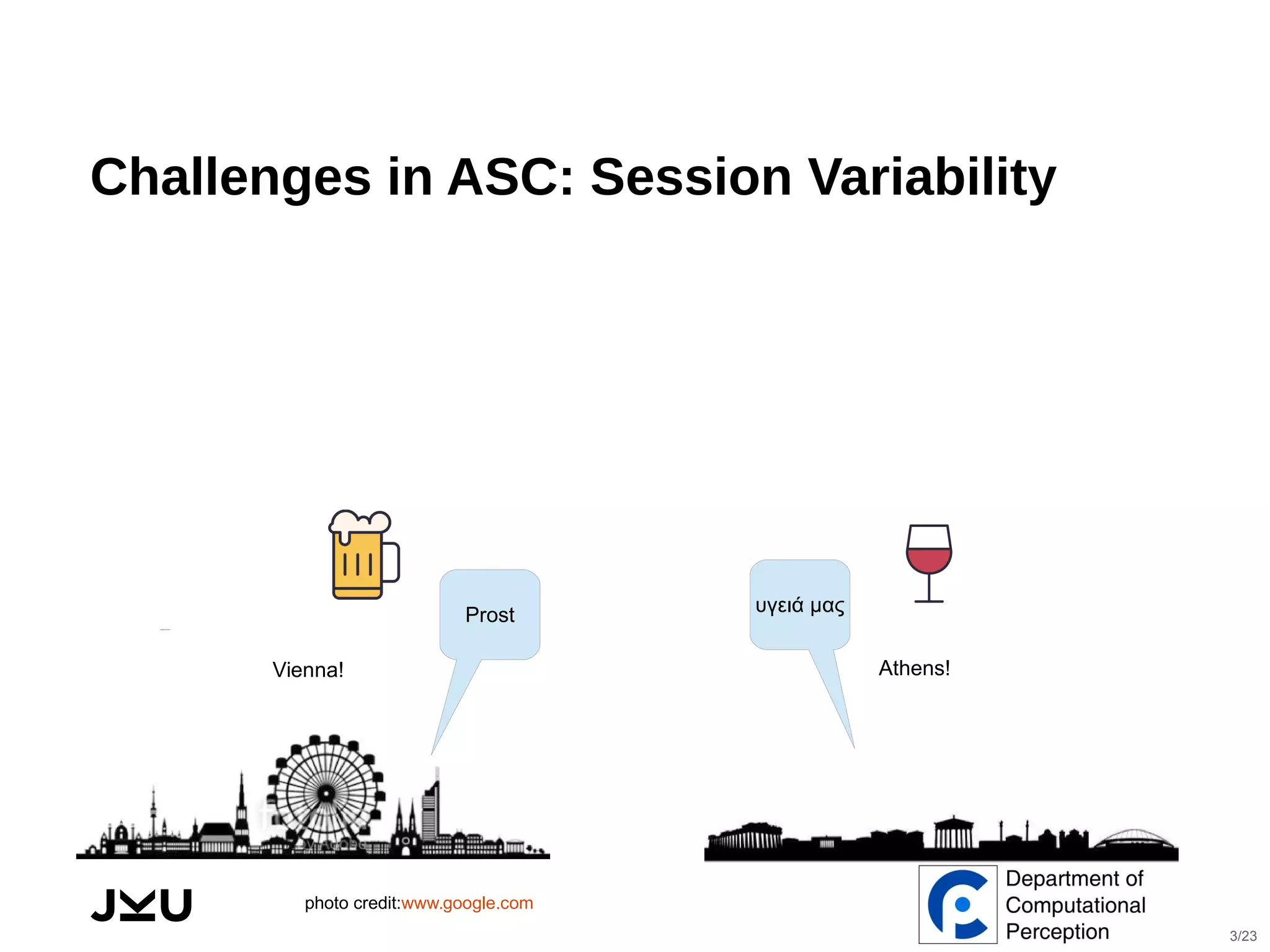
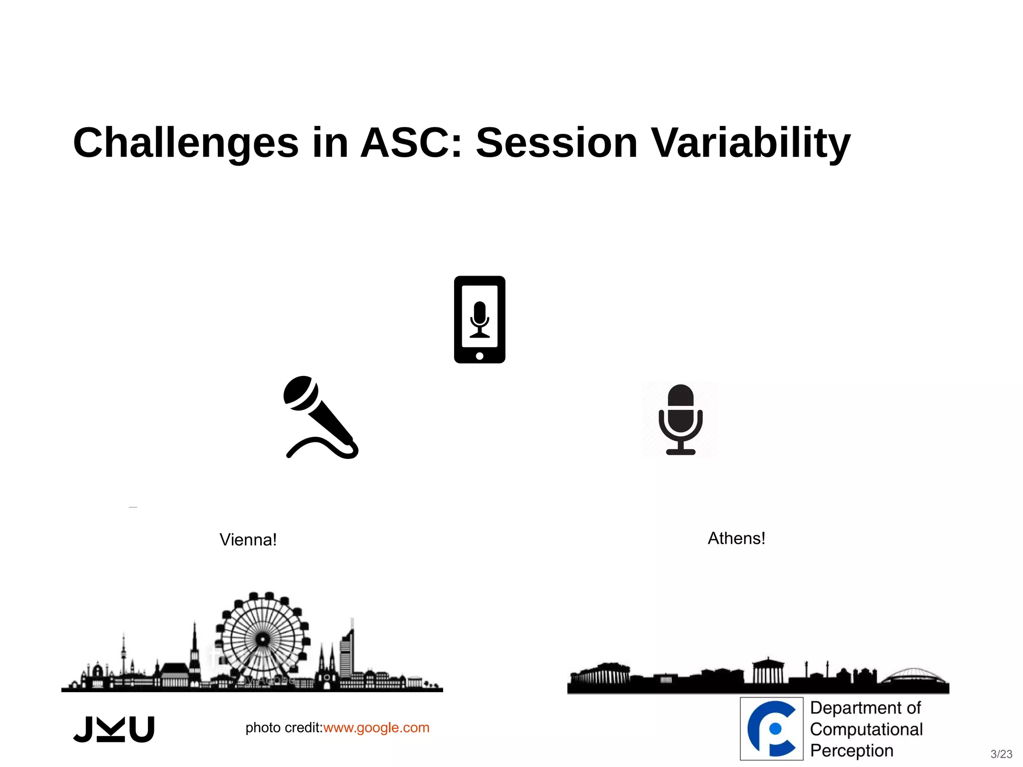
⬜ Session Variability reduction
⬜ Use of a Universal Background Model (UBM)
⬜ Better generalization due to the unsupervised methodology
⬜ Successfully applied on sequential data such as Speech and
Music
⬛ Cons:
⬜ Relying on engineered features
⬜ Limits to use specialized features for Audio Scene Analysis
because of the independence and Gaussian assumptions in FA
[1] Dehak, Najim, et al. "Front-end factor analysis for speaker verification.",2011.
[2] Elizalde, B, et al. "An i-vector based approach for audio scene detection." (2013).
5/23](https://image.slidesharecdn.com/eusipco2017hybridasc-170903075647/75/Slides-of-my-presentation-at-EUSIPCO-2017-14-2048.jpg)


![I-Vector Features
GMM Train
I-Vector
model
Sparse
statistics
Adapted GMM params = GMM params – unknown matrix . hidden factor
Learned via EM
Training
MFCCs
Many components high dimension
[1] Dehak, Najim, et al. "Front-end factor analysis for speaker verification.",2011.
[2] Elizalde, B, et al. "An i-vector based approach for audio scene detection." (2013).
[3] Kenny, Patrick, et al. "Uncertainty Modeling Without Subspace Methods For Text-Dependent
Speaker Recognition.", 2016.
low dimension
I-vector
Point estimate
low dimension
EM
8/23](https://image.slidesharecdn.com/eusipco2017hybridasc-170903075647/75/Slides-of-my-presentation-at-EUSIPCO-2017-20-2048.jpg)
![I-Vector Features
GMM
MFCCs
Sparse
statistics
I-vector
Adapted GMM params = GMM params – unknown matrix . hidden factor
Sparse
statistics
TrainingExtraction
Learned via EM
Many components
high dimension
high dimension
Train
I-Vector
model
I-vector
Point estimate
low dimension
EM
[1] Dehak, Najim, et al. "Front-end factor analysis for speaker verification.",2011.
[2] Elizalde, B, et al. "An i-vector based approach for audio scene detection." (2013).
[3] Kenny, Patrick, et al. "Uncertainty Modeling Without Subspace Methods For Text-Dependent
Speaker Recognition.", 2016.
low dimension
9/23](https://image.slidesharecdn.com/eusipco2017hybridasc-170903075647/75/Slides-of-my-presentation-at-EUSIPCO-2017-21-2048.jpg)


![Post-processing and Scoring I-Vector
Features
⬛ Length-Normalization
⬛ Within-class Covariance Normalization (WCCN)
⬛ Linear Discriminant Analysis (LDA)
⬛ Cosine Similarity:
⬜ Average I-vectors of each class in training set (Model I-vector)
⬜ Compute cosine similarity from each test I-vector to model I-
vector of each class
⬜ Pick the class with maximum similarity
[1] Garcia-Romero, D., et al. "Analysis of i-vector Length Normalization in Speaker Recognition.", 2011.
[2] Hatch, A. O.,et al. "Within-class covariance normalization for SVM-based speaker recognition.", 2006.
[3] Dehak, Najim, et al. "Cosine similarity scoring without score normalization techniques." 2010.
12/23](https://image.slidesharecdn.com/eusipco2017hybridasc-170903075647/75/Slides-of-my-presentation-at-EUSIPCO-2017-24-2048.jpg)


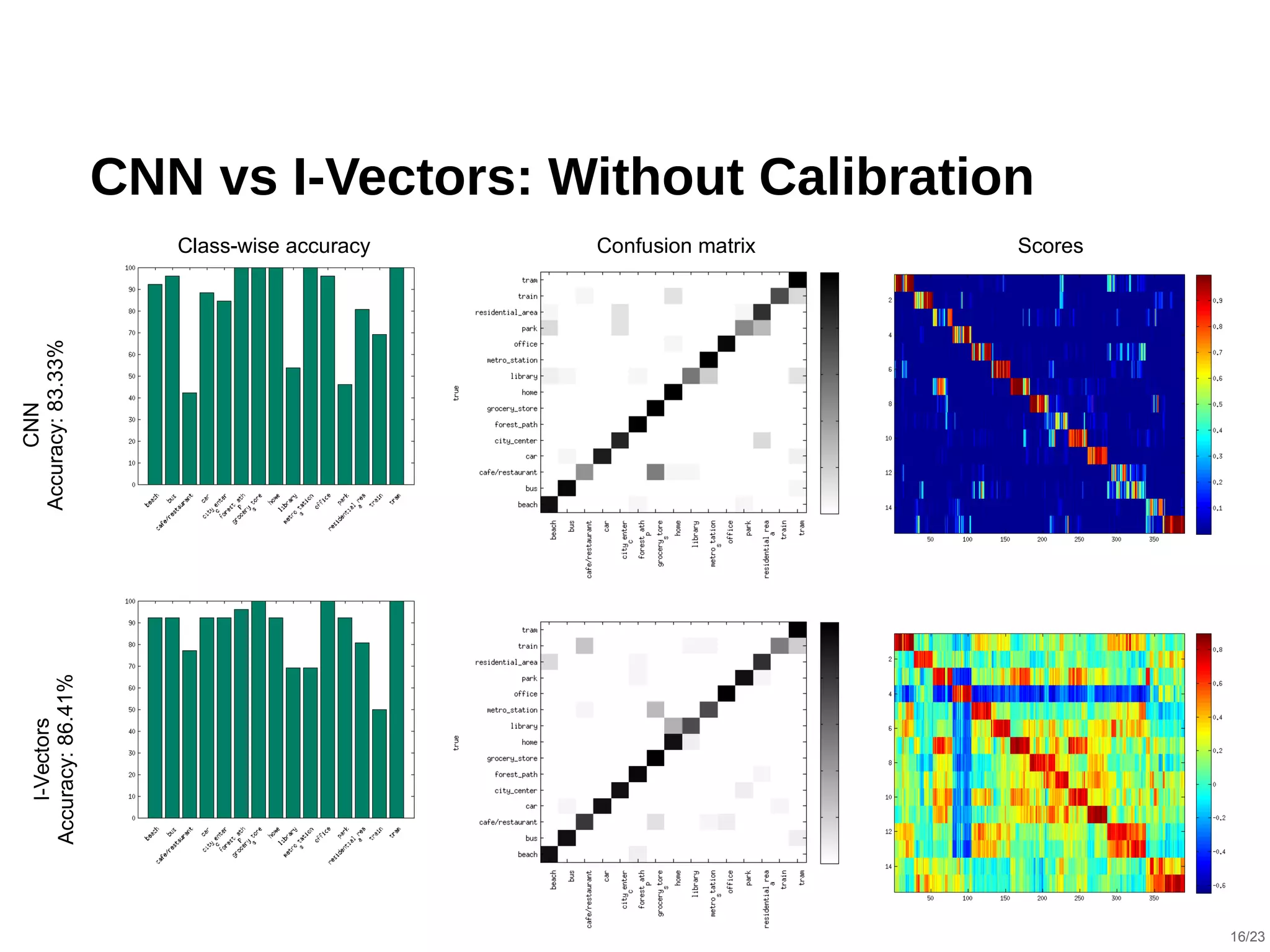
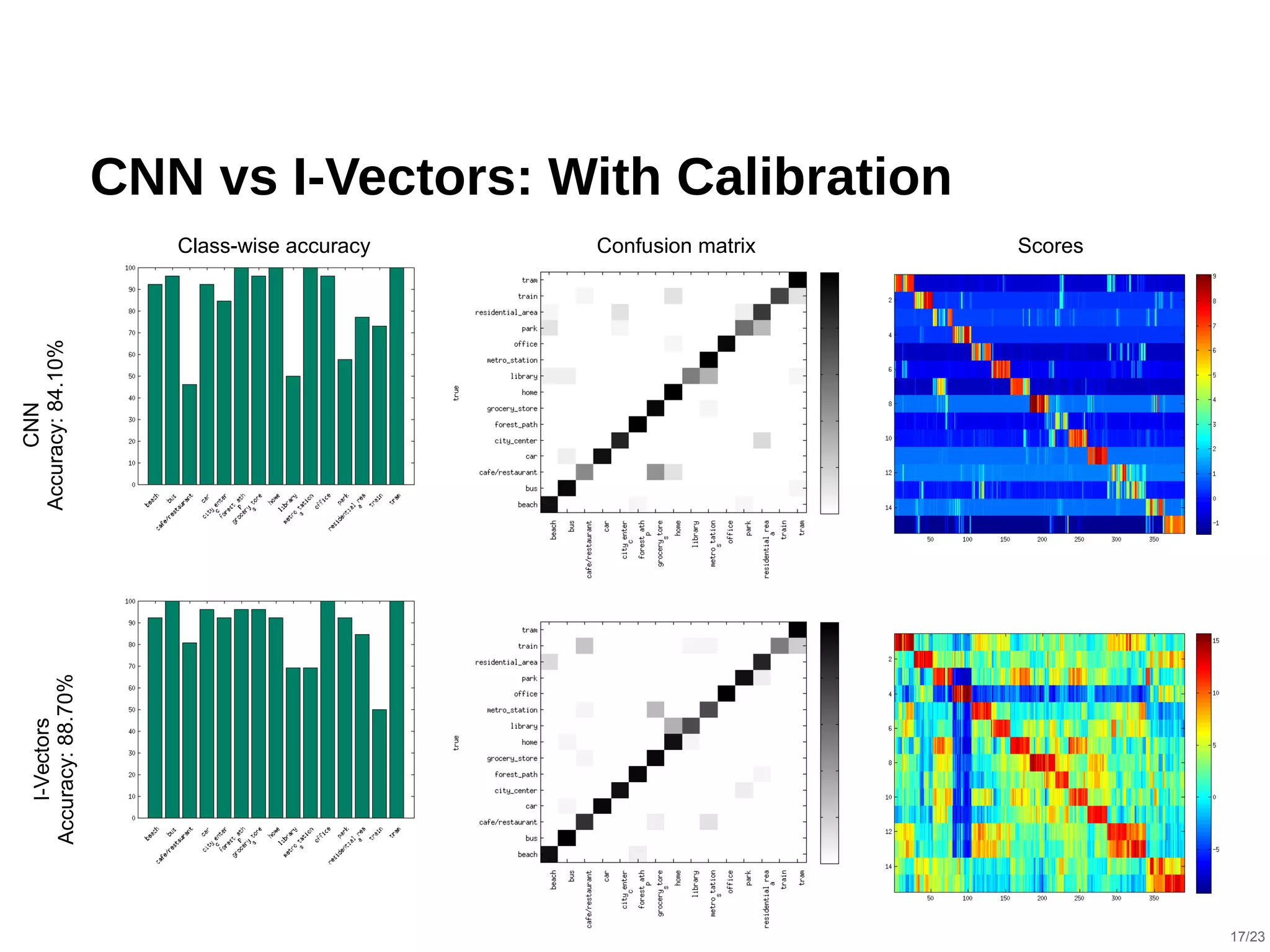
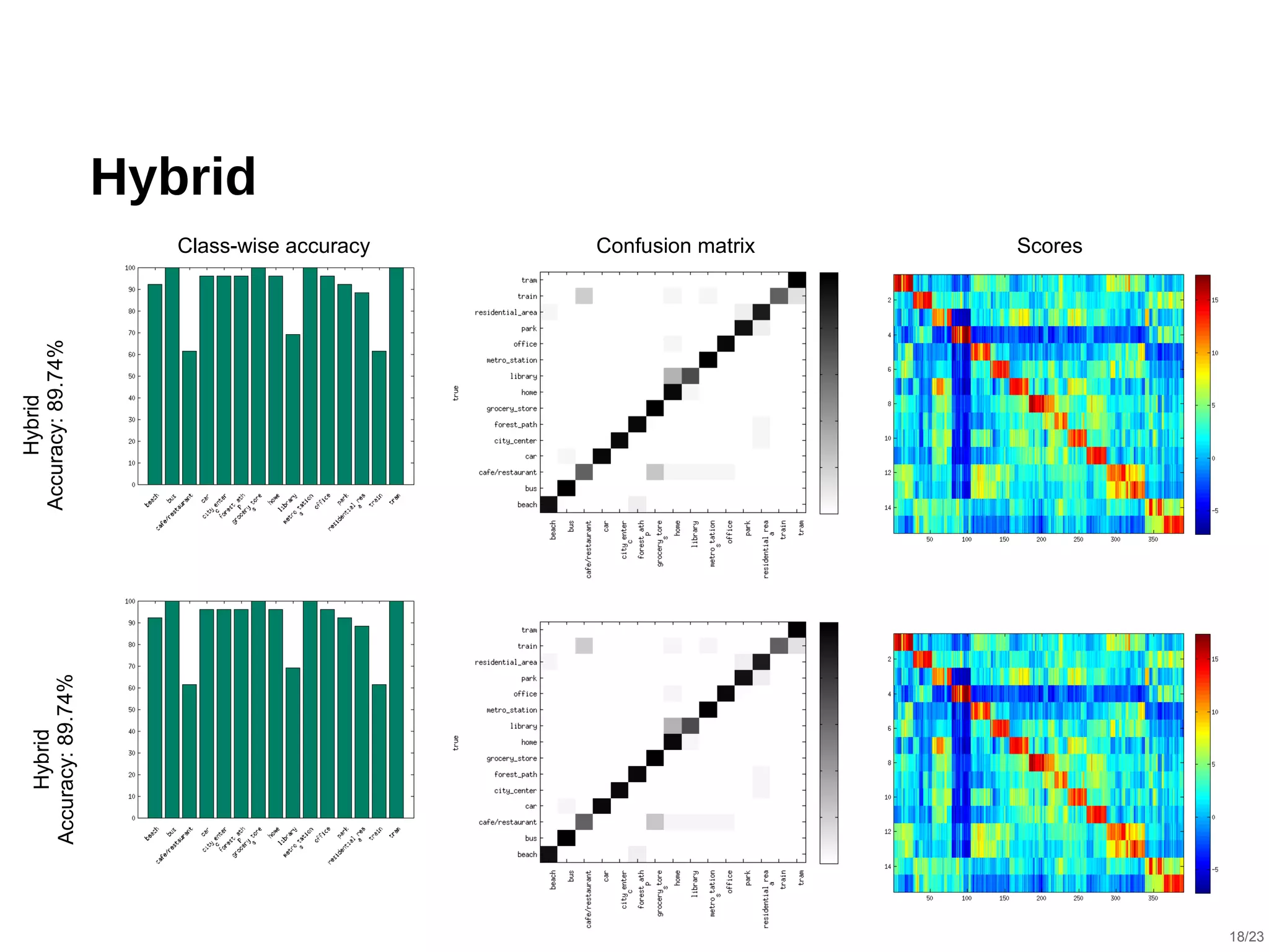

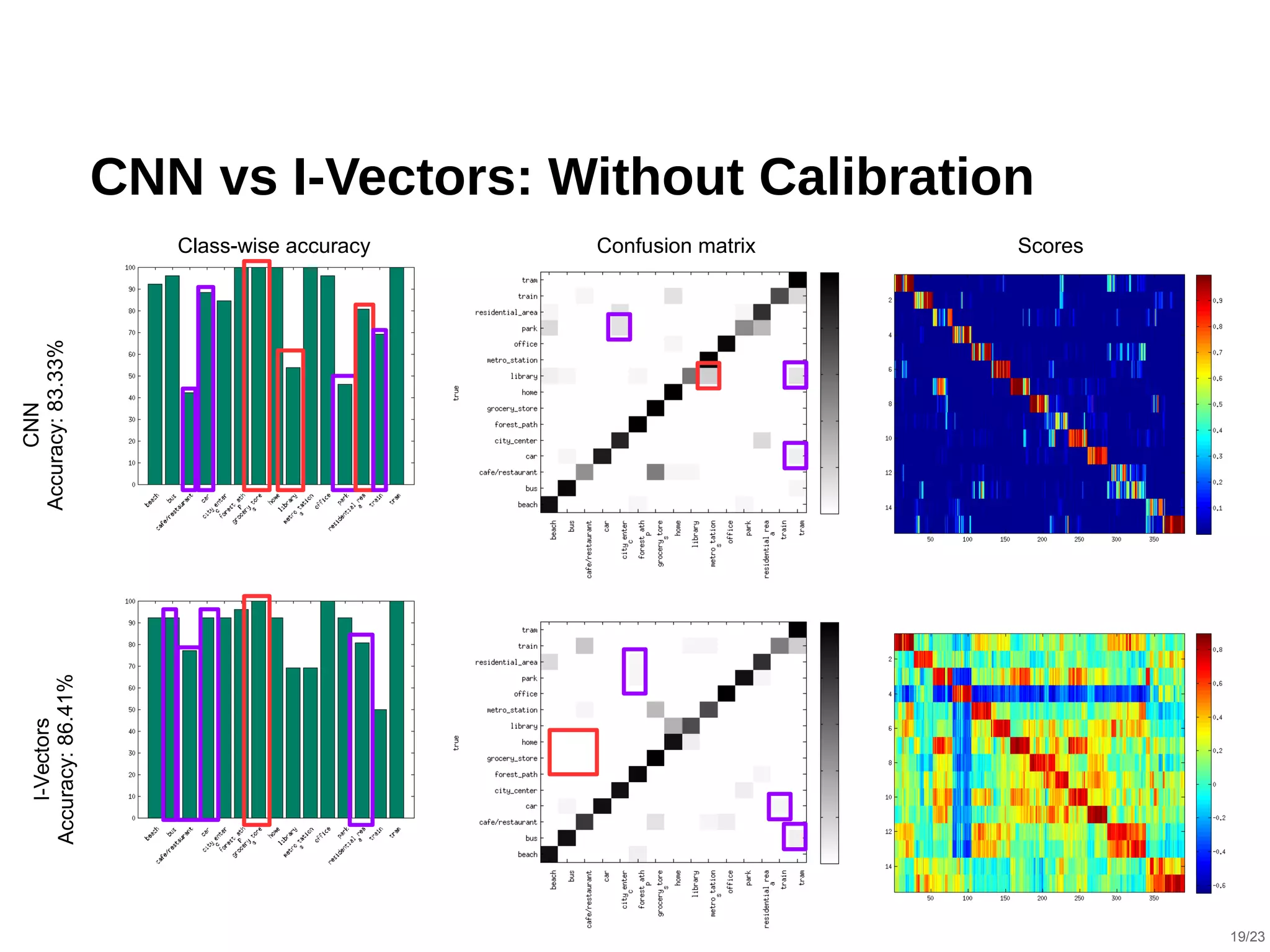
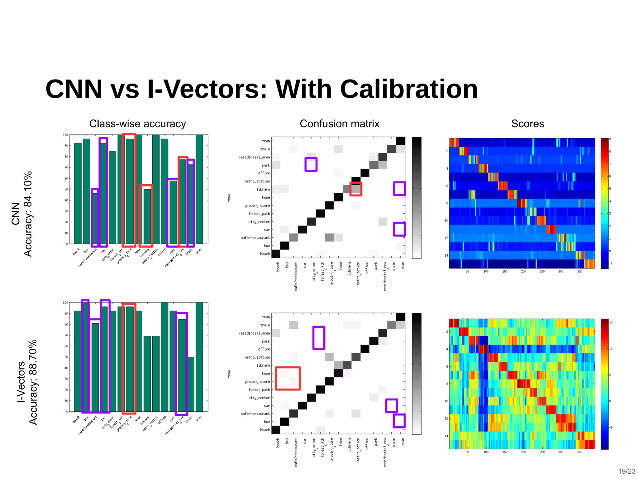


The document describes a hybrid acoustic scene classification approach that combines convolutional neural networks (CNNs) with i-vector based systems to improve classification accuracy. The hybrid model effectively handles challenges such as session variability and enhances performance through late fusion and model averaging techniques. Results indicate that the hybrid system achieves a notable accuracy increase compared to using CNNs or i-vectors alone, demonstrating their complementary nature.


