Download to read offline

![15/18
Same rainfall with different rate or mean
depth
10 12 14 16 18 20 22 24 26 28 30
0
0.2
0.4
0.6
0.8
1
1.2
1.4
α λ Ts
[cm]
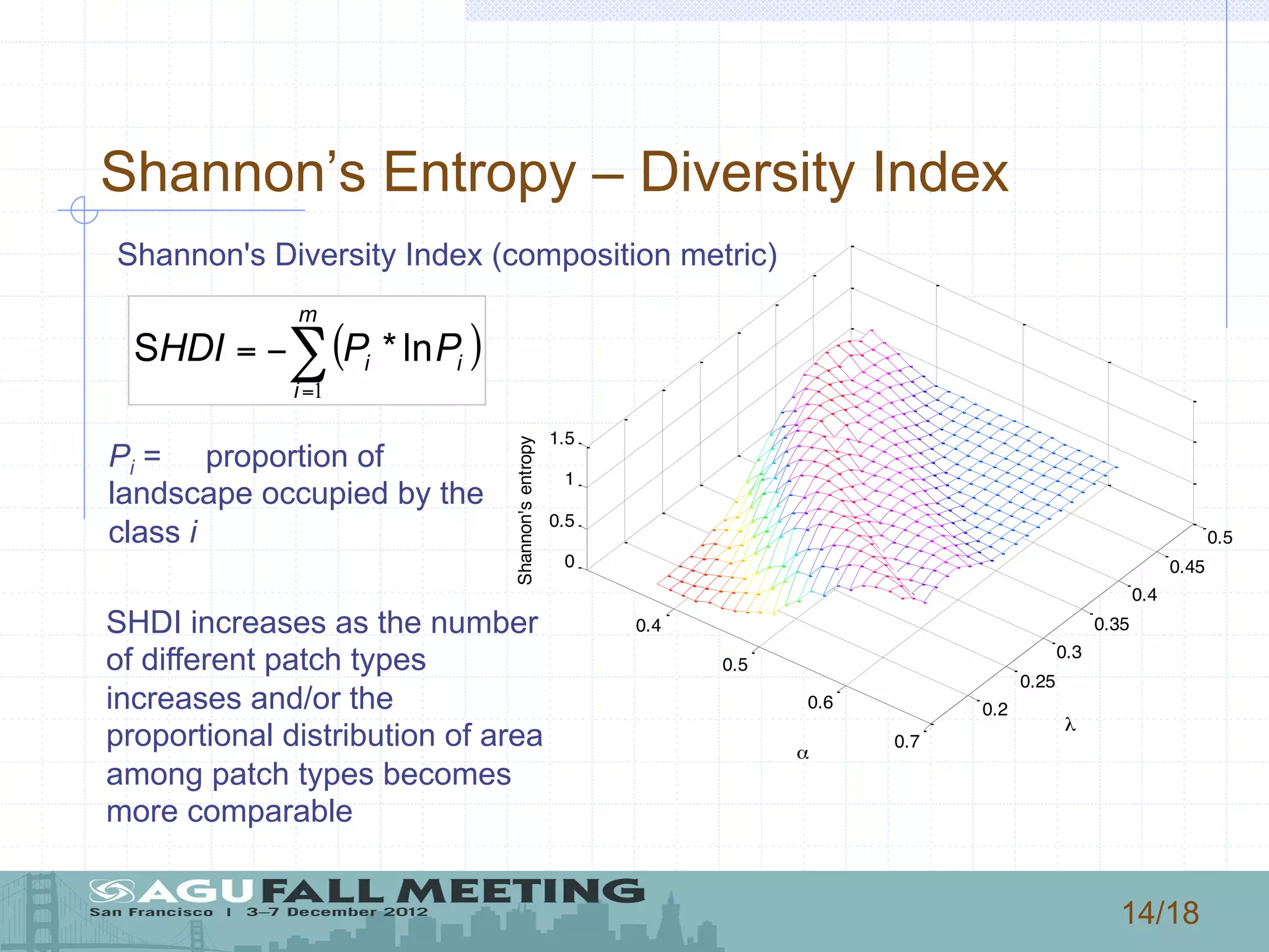
Shannon'sentropy
λ =0.224
λ =0.299
λ =0.374
λ =0.449
α =0.428
α =0.503
α =0.578
α =0.653
…changes in α provides sharper modifications of landscape.
LandscapeDiversity
Annual rainfall
Changing α
Changing λ](https://image.slidesharecdn.com/2012manfredaagu2012sanfrancisco-190114231438/75/EFFECTS-CLIMATE-CHANGE-ON-WATER-RESOURCES-AVAILABILITY-AND-VEGETATION-PATTERNS-15-2048.jpg)
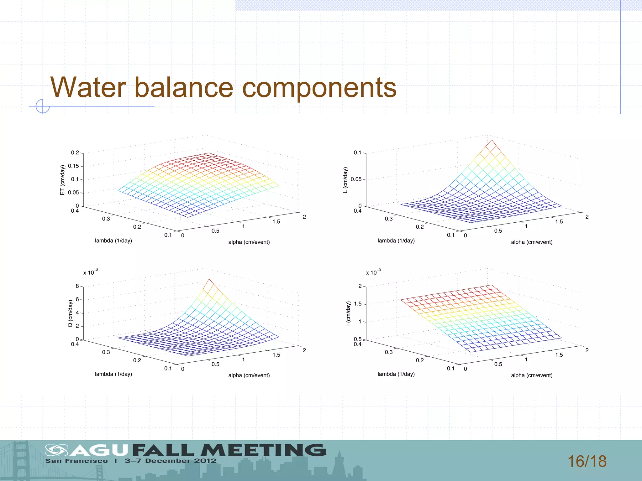


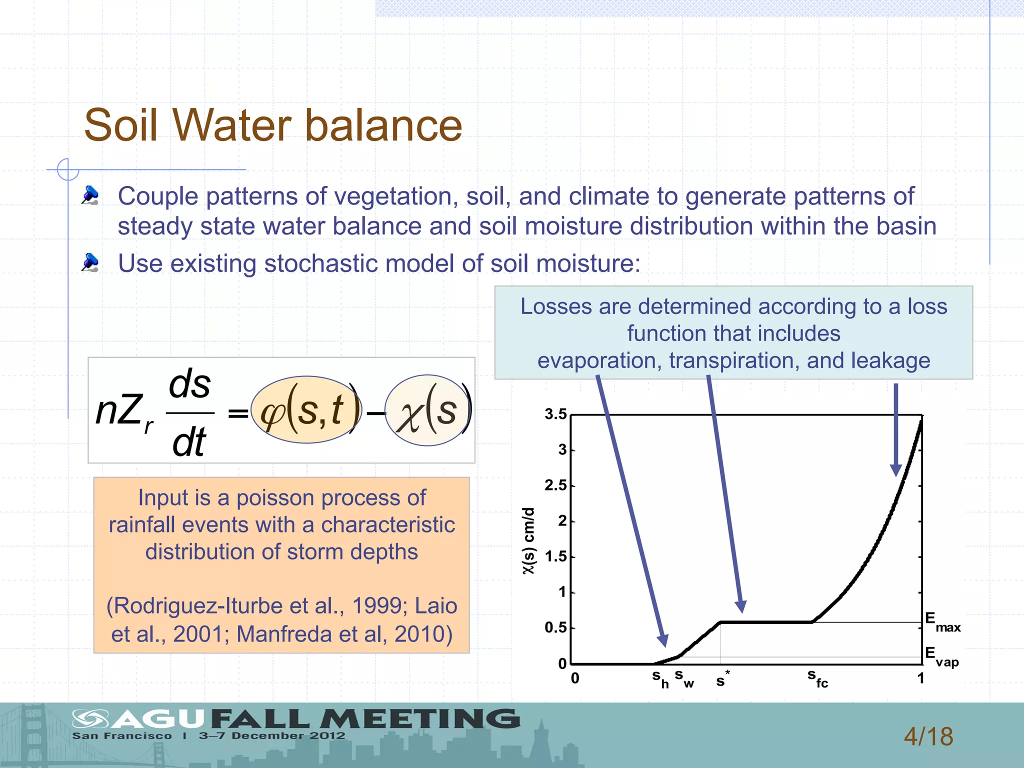
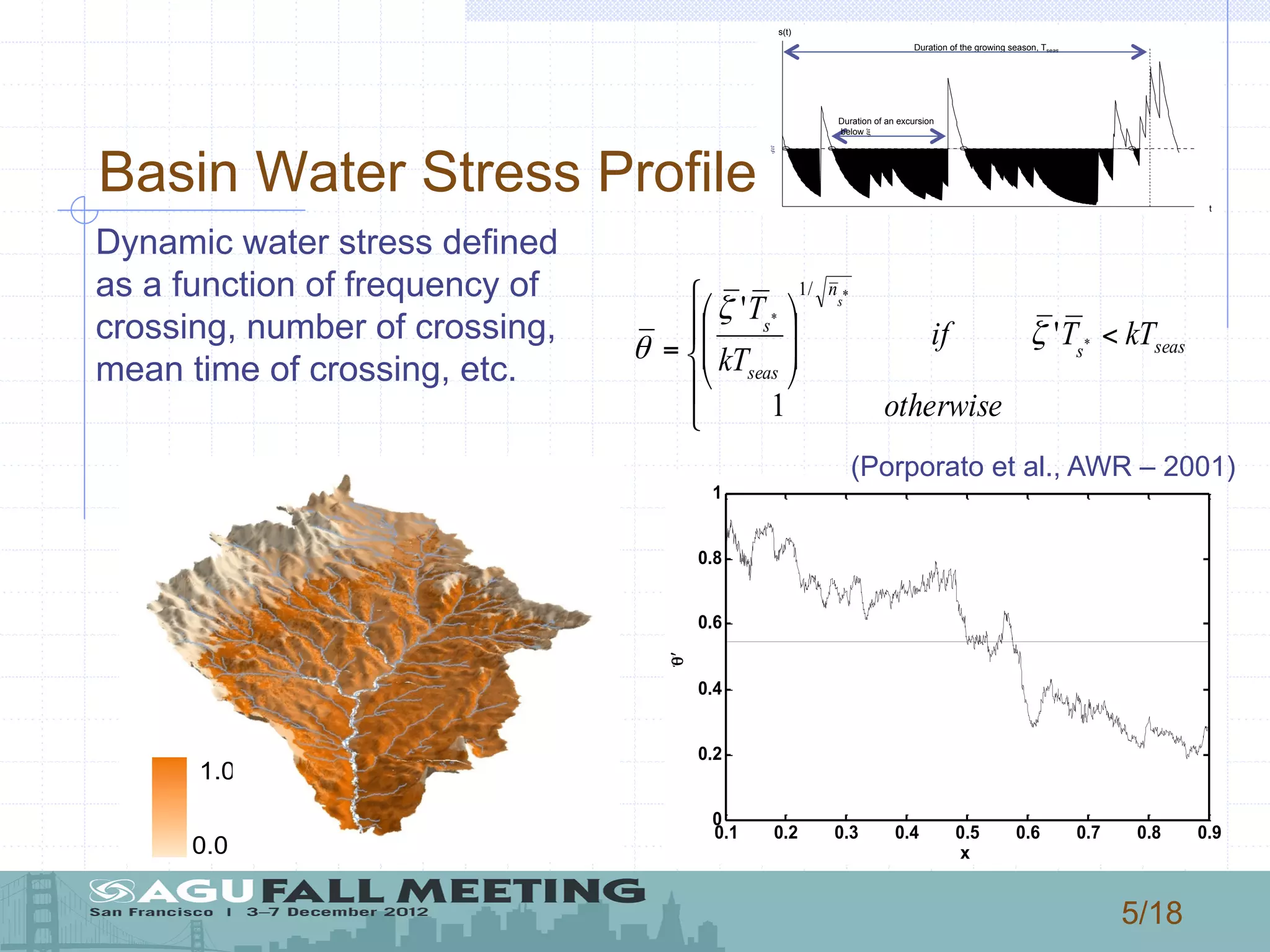
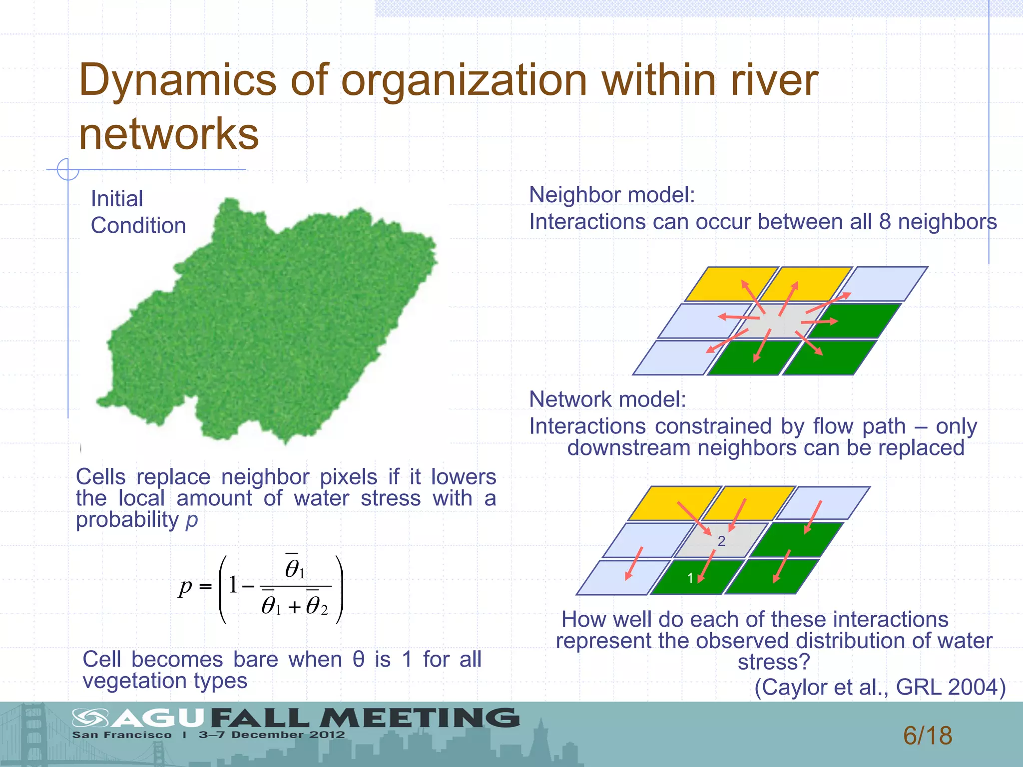
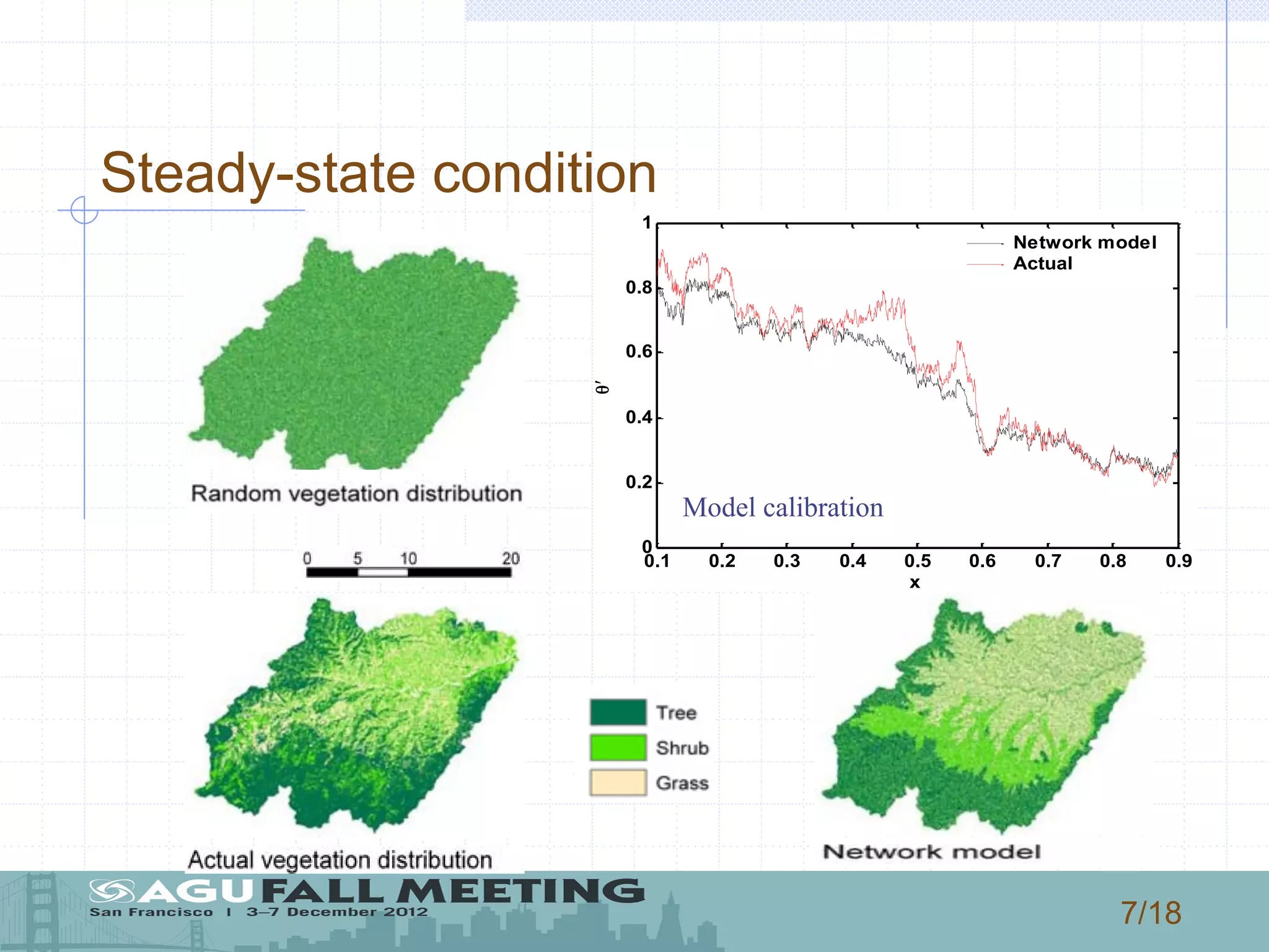
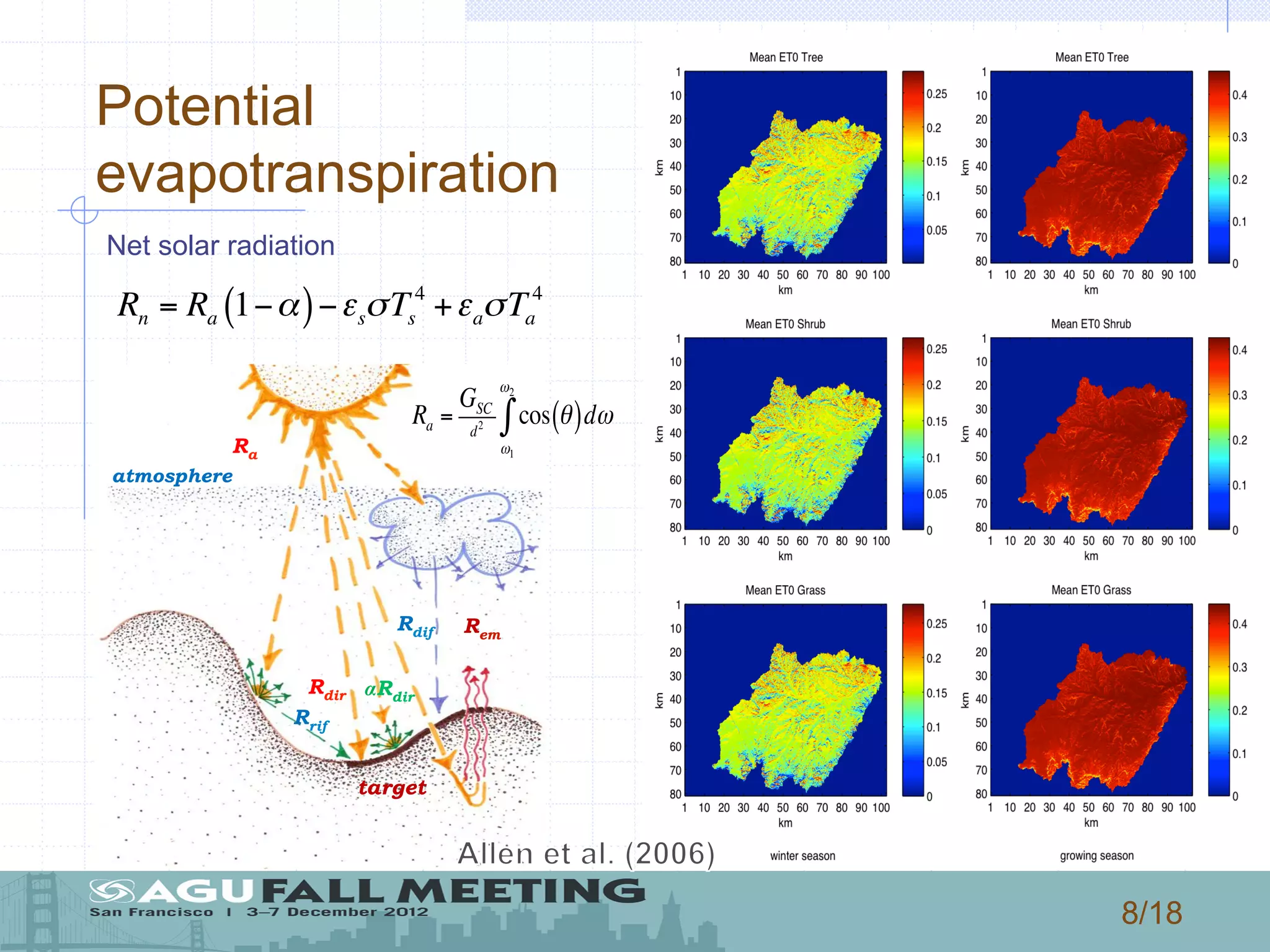
1) The document describes a model that couples patterns of vegetation, soil, and climate to generate patterns of water balance and soil moisture distribution within a basin in New Mexico. 2) The model uses a stochastic process to represent rainfall events and calculates water losses through evaporation, transpiration, and leakage to determine soil water balance. 3) The authors use the model to simulate how changes in rainfall characteristics, like rate and mean depth, could impact vegetation patterns, landscape diversity, and the water balance components of evapotranspiration, leakage, runoff, and infiltration.


