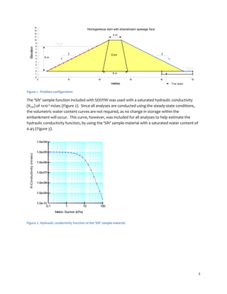
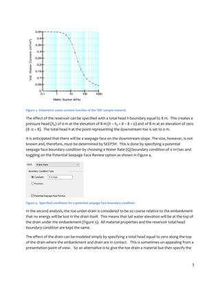
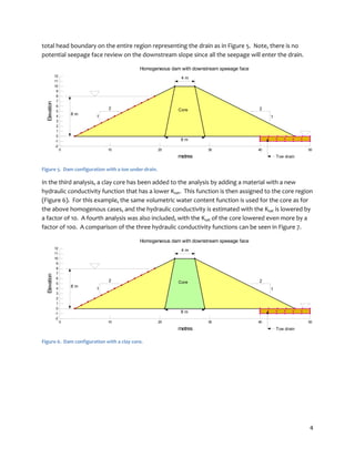
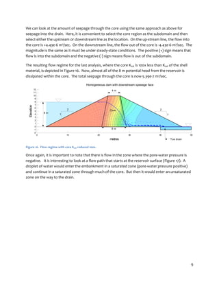
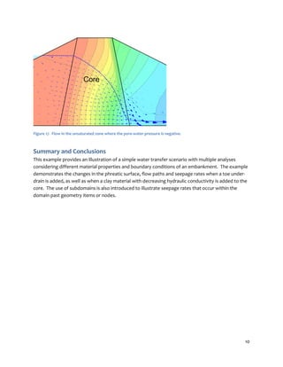
1) The document describes using SEEP/W software to model seepage through an earth dam in four scenarios: a homogeneous dam with downstream seepage, the same dam with a toe drain, and dams with a clay core where the core's hydraulic conductivity is reduced by factors of 10 and 100. 2) The first scenario models a homogeneous dam and shows a seepage face developing on the downstream slope. Adding a toe drain in the second scenario prevents a seepage face by directing all seepage into the drain. 3) Introducing a clay core with hydraulic conductivity 10 times lower than the shell materials in the third scenario causes most potential energy to dissipate in the core, as

1. 1
Seepage through an earth dam
GEO-SLOPE International Ltd. | www.geo-slope.com
1200, 700 - 6th Ave SW, Calgary, AB, Canada T2P 0T8
Main: +1 403 269 2002 | Fax: +1 888 463 2239
Introduction
Many introductory geotechnical engineering textbooks include an example explaining the scenario
of water seepage through an embankment. It is, consequently, useful to model this case with
SEEP/W, as most users will have an idea of what the solution should look like. The objective of this
example is to compare SEEP/W results with a familiar example scenario, as well as to illustrate the
analysis of various scenarios by adding multiple analyses and simply changing boundary conditions
and material properties.
Numerical Simulation
The model is a 10-m high embankment dam with 2:1 side slopes (Figure 1). Four cases will be
analyzed in this example, with an embankment impounding a reservoir that is 8 m deep. The first
case will include a single, homogeneous embankment, with seepage occurring along the
downstream face. The second case will consist of the same, homogeneous embankment, with an
under-toe drain changing the phreatic surface. Initially, the intention is to look at the homogeneous
case. The last two scenarios that will be analyzed consist of a clay core within the embankment that
has lowered hydraulic conductivities.

2. 2
11
2 2
4 m
8 m
8 m
Core
Toe drain
Homogeneous dam with downstream speeage face
metres
0 10 20 30 40 50
Elevation
-2
-1
0
1
2
3
4
5
6
7
8
9
10
11
12
13
14
Figure 1. Problem configuration.
The ‘Silt’ sample function included with SEEP/W was used with a saturated hydraulic conductivity
(Ksat) of 1x10-5 m/sec (Figure 2). Since all analyses are conducted using the steady-state conditions,
the volumetric water content curves are not required, as no change in storage within the
embankment will occur. This curve, however, was included for all analyses to help estimate the
hydraulic conductivity function, by using the ‘Silt’ sample material with a saturated water content of
0.45 (Figure 3).
X-Conductivity(m/sec)
Matric Suction (kPa)
1.0e-10
1.0e-04
1.0e-09
1.0e-08
1.0e-07
1.0e-06
1.0e-05
0.1 1001 10
Figure 2. Hydraulic conductivity function of the ‘Silt’ sample material.

3. 3
Vol.WaterContent(m³/m³)
Matric Suction (kPa)
0
0.05
0.1
0.15
0.2
0.25
0.3
0.35
0.4
0.45
0.1 10001 10 100
Figure 3. Volumetric water content function of the ‘Silt’ sample material.
The effect of the reservoir can be specified with a total head h boundary equal to 8 m. This creates a
pressure head (hp) of 0 m at the elevation of 8 m (h – hp = 8 – 8 = 0) and of 8 m at an elevation of zero
(8 -0 = 8). The total head h at the point representing the downstream toe is set to 0 m.
It is anticipated that there will be a seepage face on the downstream slope. The size, however, is not
known and, therefore, must be determined by SEEP/W. This is done by specifying a potential
seepage face boundary condition by choosing a Water Rate (Q) boundary condition of 0 m3/sec and
toggling on the Potential Seepage Face Review option as shown in Figure 4.
Figure 4. Specified conditions for a potential seepage face boundary condition.
In the second analysis, the toe under-drain is considered to be so coarse relative to the embankment
that no energy will be lost in the drain itself. This means that tail water elevation will be at the top of
the drain under the embankment (Figure 5). All material properties and the reservoir total head
boundary condition are kept the same.
The effect of the drain can be modeled simply by specifying a total head equal to zero along the top
of the drain where the embankment and drain are in contact. This is sometimes un-appealing from a
presentation point of view. So an alternative is to give the toe drain a material but then specify the

4. 4
total head boundary on the entire region representing the drain as in Figure 5. Note, there is no
potential seepage face review on the downstream slope since all the seepage will enter the drain.
11
2 2
4 m
8 m
8 m
Core
Toe drain
Homogeneous dam with downstream speeage face
metres
0 10 20 30 40 50
Elevation
-2
-1
0
1
2
3
4
5
6
7
8
9
10
11
12
Figure 5. Dam configuration with a toe under-drain.
In the third analysis, a clay core has been added to the analysis by adding a material with a new
hydraulic conductivity function that has a lower Ksat. This function is then assigned to the core region
(Figure 6). For this example, the same volumetric water content function is used for the core as for
the above homogenous cases, and the hydraulic conductivity is estimated with the Ksat is lowered by
a factor of 10. A fourth analysis was also included, with the Ksat of the core lowered even more by a
factor of 100. A comparison of the three hydraulic conductivity functions can be seen in Figure 7.
11
2 2
4 m
8 m
8 m
Core
Toe drain
Homogeneous dam with downstream speeage face
metres
0 10 20 30 40 50
Elevation
-2
-1
0
1
2
3
4
5
6
7
8
9
10
11
12
Figure 6. Dam configuration with a clay core.

5. 5
Silt K function
Silt K function 100x
less
Silt K function 10x
less
X-Conductivity(m/sec)
Matric Suction (kPa)
1.0e-04
1.0e-11
1.0e-10
1.0e-09
1.0e-08
1.0e-07
1.0e-06
1.0e-05
0.1 1001 10
Figure 7. Comparison of the core material hydraulic conductivity functions to the embankment.
Results and Discussion
Figure 8 presents the resulting steady-state, homogenous condition without a toe under-drain. The
dashed line is a line where the pore-water pressure is zero. The contours shown are total head
contours or equipotential lines (the energy potential along these lines is a constant). As expected, a
seepage face is present on the downstream slope.
3
4
5
6
7
11
2 2
4 m
8 m
8 m
Core
Toe drain
Homogeneous dam with downstream speeage face
metres
0 10 20 30 40 50
Elevation
-2
-1
0
1
2
3
4
5
6
7
8
9
10
11
12
Figure 8. Equipotential lines for the homogeneous case.
Figure 9 shows the flow vectors, which provide a sense of direction and rate of flow. The longest
vectors indicate the areas of highest flow rate. Where the flow is extremely low, such as in the crest
and upstream toe areas, the vectors become so small that they are not visible. Notice the vectors
above the zero-pressure line, which represent the flow in the capillary zone. The vectors also reveal
the flow out of the domain occurring along the seepage face.

6. 6
11
2 2
4 m
8 m
8 m
Core
Toe drain
Homogeneous dam with downstream speeage face
metres
0 10 20 30 40 50
Elevation
-2
-1
0
1
2
3
4
5
6
7
8
9
10
11
12
Figure 9. Flow vectors for the homogeneous case.
Figure 10 shows three flow paths that were added. Note, these are NOT flow channels as in a flow
net, but indicate paths that a droplet of water will follow through the embankment. Even though
they do not represent flow channels, they nonetheless make it possible to provide the appearance of
a flow net – at least in part.
11
2 2
4 m
8 m
8 m
Core
Toe drain
Homogeneous dam with downstream speeage face
metres
0 10 20 30 40 50
Elevation
-2
-1
0
1
2
3
4
5
6
7
8
9
10
11
12
Figure 10. Flow paths for the homogeneous case.
As in a flow net, the flow paths cross the equipotential lines at right-angles. The flow path above the
zero-pressure line represents the flow in the tension-saturated capillary zone.
The quantity of seepage through the dam can be determined with the Draw Graph command.
Selecting the options as in Figure 11 for the downstream face gives a graph with one data point. The
total seepage rate is -1.222e-5 m3/sec. The negative sign indicates flow is occurring out of the domain.

7. 7
Figure 11. Settings for a seepage quantity graph.
Figure 12 shows the flow regime with the under-drain added to the homogeneous case. As
expected, the drain prevents the development of a seepage face on the downstream side of the
dam. All of the seepage, instead, goes into the drain.
11
2 2
4 m
8 m
8 m
Core
Toe drain
Homogeneous dam with downstream speeage face
metres
0 10 20 30 40 50
Elevation
-2
-1
0
1
2
3
4
5
6
7
8
9
10
11
12
Figure 12. Flow regime with a toe under-drain.
Notice that a significant amount of seepage flows into the drain through the capillary zone where
the pore-water pressure is negative. Figure 13 shows the amount of flow into the drain at each of
the nodes along the top of the drain. The total into the drain is 1.53e-5 m3/sec.
The graph in Figure 13 is created using a subdomain and then selecting the geometry line along the
top of the drain as the location (Figure 14). In this case, the subdomain can be selected by simply
clicking on the geometry line between the embankment and the drain, causing all connecting
elements to be chosen for the subdomain. It is important to note that most of the seepage into the
drain arrives through a zone where the pore-water pressure is negative.

8. 8
Seepage quantityWaterRate(m³/sec)
X(m)
-2e-006
-4e-006
-6e-006
-8e-006
-1e-005
-1.2e-005
0
2e-006
40 41 42 43 44 45 46 47
Figure 13. Flow into the drain at each node along the top of the drain.
Figure 14. Choosing geometry item for subdomain.
Figure 15 shows the flow regime for the third case, where the Ksat of the core is 10x less than Ksat of
the shell material. The large drop in the zero-pressure line within the core indicates that much of the
potential energy is dissipated in the core.
11
2 2
4 m
8 m
8 m
Core
Toe drain
Homogeneous dam with downstream speeage face
metres
0 10 20 30 40 50
Elevation
-2
-1
0
1
2
3
4
5
6
7
8
9
10
11
12
Figure 15. Flow regime with core Ksat reduced 10x.

9. 9
We can look at the amount of seepage through the core using the same approach as above for
seepage into the drain. Here, it is convenient to select the core region as the subdomain and then
select either the upstream or downstream line as the location. On the up-stream line, the flow into
the core is +4.43e-6 m3/sec. On the downstream line, the flow out of the core is -4.43e-6 m3/sec. The
magnitude is the same as it must be under steady-state conditions. The positive (+) sign means that
flow is into the subdomain and the negative (-) sign means flow is out of the subdomain.
The resulting flow regime for the last analysis, where the core Ksat is 100x less than Ksat of the shell
material, is depicted in Figure 16. Now, almost all of the 8 m potential head from the reservoir is
dissipated within the core. The total seepage through the core is now 5.39e-7 m3/sec.
11
2 2
4 m
8 m
8 m
Core
Toe drain
Homogeneous dam with downstream speeage face
metres
0 10 20 30 40 50
Elevation
-2
-1
0
1
2
3
4
5
6
7
8
9
10
11
12
Figure 16. Flow regime with core Ksat reduced 100x.
Once again, it is important to note that there is flow in the zone where the pore-water pressure is
negative. It is interesting to look at a flow path that starts at the reservoir surface (Figure 17). A
droplet of water would enter the embankment in a saturated zone (pore-water pressure positive)
and continue in a saturated zone through much of the core. But then it would enter an unsaturated
zone on the way to the drain.

10. 10
Core
Figure 17. Flow in the unsaturated zone where the pore-water pressure is negative.
Summary and Conclusions
This example provides an illustration of a simple water transfer scenario with multiple analyses
considering different material properties and boundary conditions of an embankment. The example
demonstrates the changes in the phreatic surface, flow paths and seepage rates when a toe under-
drain is added, as well as when a clay material with decreasing hydraulic conductivity is added to the
core. The use of subdomains is also introduced to illustrate seepage rates that occur within the
domain past geometry items or nodes.