About time to study genetics

1. Introduction
• Definition
• Genetics is the study of inheritance in all of its
manifestations, from the distribution of human traits in a family
pedigree to the biochemistry of the genetic material in our
chromosomes, deoxyribonucleic acid (DNA).
• Genetics includes the rules of inheritance in cells, individuals,
and populations and the molecular mechanisms by which
genes control the growth, development, & appearance of an
organism.

2. Three major areas of Genetics
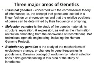
• Classical genetics - concerned with the chromosomal theory
of inheritance; i.e. the concept that genes are located in a
linear fashion on chromosomes and that the relative positions
of genes can be determined by their frequency in offspring.
• Molecular genetics is the study of the genetic material: its
structure, replication, & expression, as well as the information
revolution emanating from the discoveries of recombinant DNA
techniques (genetic engineering, including the Human
Genome Project).
• Evolutionary genetics is the study of the mechanisms of
evolutionary change, or changes in gene frequencies in
populations. Darwin’s concept of evolution by natural selection
finds a firm genetic footing in this area of the study of
inheritance.

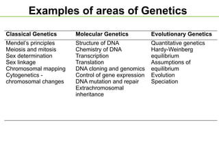
3. Examples of areas of Genetics
Classical Genetics Molecular Genetics Evolutionary Genetics
Mendel’s principles
Meiosis and mitosis
Sex determination
Sex linkage
Chromosomal mapping
Cytogenetics -
chromosomal changes
Structure of DNA
Chemistry of DNA
Transcription
Translation
DNA cloning and genomics
Control of gene expression
DNA mutation and repair
Extrachromosomal
inheritance
Quantitative genetics
Hardy-Weinberg
equilibrium
Assumptions of
equilibrium
Evolution
Speciation

4. Introduction
• Evolution is the change in allelic frequencies in a
population over time.
• Evolution is the result of natural selection (Charles
Darwin).
• Evolution takes place in populations of organisms
• In the 1920s &1930s, geneticists; Sewall Wright, R. A.
Fisher, and J. B. S. Haldane, provided algebraic
models to describe evolutionary processes.
• The marriage of Darwinian theory and population
genetics has been termed neo-Darwinism.

5. Introduction
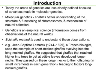
• Today the areas of genetics are less clearly defined because
of advances made in molecular genetics.
• Molecular genetics - enables better understanding of the
structure & functioning of chromosomes, & mechanism of
natural selection.
• Genetics is an empirical science (information comes from
observations of the natural world).
• Scientific method is used to understand these observations.
• e.g., Jean-Baptiste Lamarck (1744–1829), a French biologist,
used the example of short-necked giraffes evolving into the
long-necked giraffes. He suggested that giraffes that reached
higher into trees to get at edible leaves developed longer
necks. They passed on these longer necks to their offspring (in
small increments in each generation), leading to today’s long-
necked giraffes.

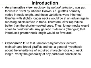
6. • An alternative view, evolution by natural selection, was put
forward in 1859 by Charles Darwin. i.e. giraffes normally
varied in neck length, and these variations were inherited.
Giraffes with slightly longer necks would be at an advantage in
reaching edible leaves in trees. Therefore, over reproduce
better than the shorter-necked ones. Thus, longer necks would
come to predominate. Any genetic mutations (changes) that
introduced greater neck length would be favoured.
• Experiment 1: To test Lamarck’s hypothesis: acquire,
maintain and breed giraffes and test a general hypothesis
about the inheritance of acquired characteristics e.g. neck
length. Verify the generality of any particular conclusions.
Introduction

7. Three major areas of Genetics
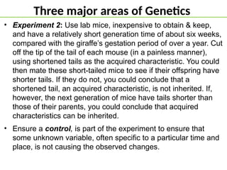
• Experiment 2: Use lab mice, inexpensive to obtain & keep,
and have a relatively short generation time of about six weeks,
compared with the giraffe’s gestation period of over a year. Cut
off the tip of the tail of each mouse (in a painless manner),
using shortened tails as the acquired characteristic. You could
then mate these short-tailed mice to see if their offspring have
shorter tails. If they do not, you could conclude that a
shortened tail, an acquired characteristic, is not inherited. If,
however, the next generation of mice have tails shorter than
those of their parents, you could conclude that acquired
characteristics can be inherited.
• Ensure a control, is part of the experiment to ensure that
some unknown variable, often specific to a particular time and
place, is not causing the observed changes.

8. Population Genetics
• Evolution can be defined as a change in gene frequencies
through time.
• Population genetics tracks the fate, across generations, of
Mendelian genes in populations.
• Population genetics is concerned with whether a particular
allele or genotype will become more or less common over
time, and WHY.

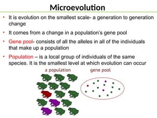
9. Microevolution
• It is evolution on the smallest scale- a generation to generation
change
• It comes from a change in a population’s gene pool
• Gene pool- consists of all the alleles in all of the individuals
that make up a population
• Population – is a local group of individuals of the same
species. It is the smallest level at which evolution can occur

10. Gene pools
• A gene pool is like a reservoir from which the next generation
of individuals gets their genes
• It is the raw material for evolution
• Gene pools reflect the variation among individuals that is
largely a result of sexual recombination
• Meiosis and fertilization shuffle alleles and deal out fresh
combinations to the offspring

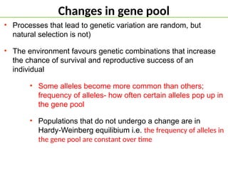
12. Changes in gene pool
• Processes that lead to genetic variation are random, but
natural selection is not)
• The environment favours genetic combinations that increase
the chance of survival and reproductive success of an
individual
• Some alleles become more common than others;
frequency of alleles- how often certain alleles pop up in
the gene pool
• Populations that do not undergo a change are in
Hardy-Weinberg equilibium i.e. the frequency of alleles in
the gene pool are constant over time

13. Population structure
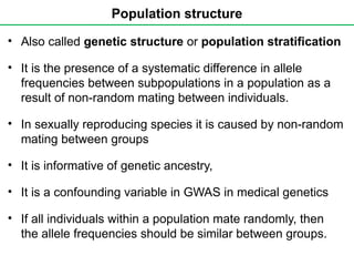
• Also called genetic structure or population stratification
• It is the presence of a systematic difference in allele
frequencies between subpopulations in a population as a
result of non-random mating between individuals.
• In sexually reproducing species it is caused by non-random
mating between groups
• It is informative of genetic ancestry,
• It is a confounding variable in GWAS in medical genetics
• If all individuals within a population mate randomly, then
the allele frequencies should be similar between groups.

14. Hardy Weinberg equilibrium
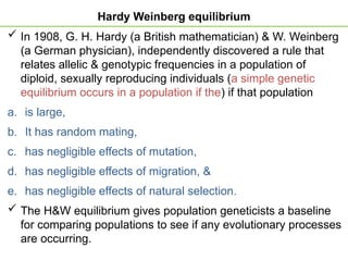
 In 1908, G. H. Hardy (a British mathematician) & W. Weinberg
(a German physician), independently discovered a rule that
relates allelic & genotypic frequencies in a population of
diploid, sexually reproducing individuals (a simple genetic
equilibrium occurs in a population if the) if that population
a. is large,
b. It has random mating,
c. has negligible effects of mutation,
d. has negligible effects of migration, &
e. has negligible effects of natural selection.
 The H&W equilibrium gives population geneticists a baseline
for comparing populations to see if any evolutionary processes
are occurring.

15. • A statement to describe the equilibrium condition:
 If the assumptions are met, the population will not experience
changes in allelic frequencies,
 and these allelic frequencies will accurately predict the
frequencies of genotypes (allelic combinations in individuals,
e.g., AA, Aa, or aa) in the population.
 A; a
Hardy Weinberg equilibrium assumptions

16. H-W rule has 3 aspects
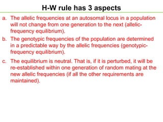
a. The allelic frequencies at an autosomal locus in a population
will not change from one generation to the next (allelic-
frequency equilibrium).
b. The genotypic frequencies of the population are determined
in a predictable way by the allelic frequencies (genotypic-
frequency equilibrium).
c. The equilibrium is neutral. That is, if it is perturbed, it will be
re-established within one generation of random mating at the
new allelic frequencies (if all the other requirements are
maintained).

17. H-W rule assumptions
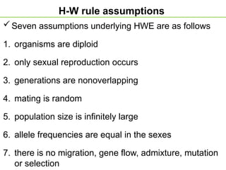
Seven assumptions underlying HWE are as follows
1. organisms are diploid
2. only sexual reproduction occurs
3. generations are nonoverlapping
4. mating is random
5. population size is infinitely large
6. allele frequencies are equal in the sexes
7. there is no migration, gene flow, admixture, mutation
or selection

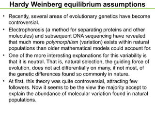
18. Hardy Weinberg equilibrium assumptions
• Recently, several areas of evolutionary genetics have become
controversial.
• Electrophoresis (a method for separating proteins and other
molecules) and subsequent DNA sequencing have revealed
that much more polymorphism (variation) exists within natural
populations than older mathematical models could account for.
• One of the more interesting explanations for this variability is
that it is neutral. That is, natural selection, the guiding force of
evolution, does not act differentially on many, if not most, of
the genetic differences found so commonly in nature.
• At first, this theory was quite controversial, attracting few
followers. Now it seems to be the view the majority accept to
explain the abundance of molecular variation found in natural
populations.

19. Evolutionary Genetics
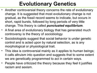
• Another controversial theory concerns the rate of evolutionary
change. It is suggested that most evolutionary change is not
gradual, as the fossil record seems to indicate, but occurs in
short, rapid bursts, followed by long periods of very little
change. This theory is called punctuated equilibrium.
• A final area of evolutionary biology that has generated much
controversy is the theory of sociobiology.
• Sociobiologists suggest that social behavior is under genetic
control and is acted upon by natural selection, as is any
morphological or physiological trait.
• This idea is controversial mainly as it applies to human beings;
it calls altruism into question and suggests that to some extent
we are genetically programmed to act in certain ways.
• People have criticized the theory because they feel it justifies
racism and sexism.

20. 2.2 Terms
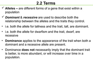
 Alleles – are different forms of a gene that exist within a
population
 Dominant & recessive are used to describe both the
relationship between the alleles and the traits they control.
• i.e. both the allele for tallness and the trait, tall, are dominant.
• i.e. both the allele for dwarfism and the trait, dwarf, are
recessive
• Dominance applies to the appearance of the trait when both a
dominant and a recessive allele are present.
• Dominance does not necessarily imply that the dominant trait
is better, is more abundant, or will increase over time in a
population.

21. 2.2 Terms
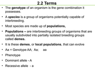
• The genotype of an organism is the gene combination it
possesses.
• A species is a group of organisms potentially capable of
interbreeding.
• Most species are made up of populations,
• Populations – are interbreeding groups of organisms that are
usually subdivided into partially isolated breeding groups
called demes.
• It is these demes, or local populations, that can evolve
• Aa = Genotype AA; Aa; aa
• Phenotype
• Dominant allele - A
• Recessive allele - a

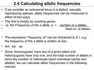
22. 2.4 Calculating allelic frequencies
• If we consider an autosomal locus in a diploid, sexually
reproducing species, allelic frequencies can be measured in
either of two ways.
• The first is simply by counting genes
• i.e, the Frequency of the a allele, q, = number of a alleles
• Total no. of alleles
• The expression “frequency of” can be shortened to f( ). e.g.,
the frequency of the a allele is written as f(a).
• AA; Aa; aa
• Since ‘homozygotes’ have two of a given allele and
heterozygotes have only one, and the total number of alleles is
twice the number of individuals (each individual carries two
alleles), we can calculate allelic frequencies in the following
manner.

23. 2.4 Calculating allelic frequencies
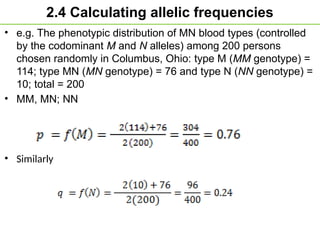
• e.g. The phenotypic distribution of MN blood types (controlled
by the codominant M and N alleles) among 200 persons
chosen randomly in Columbus, Ohio: type M (MM genotype) =
114; type MN (MN genotype) = 76 and type N (NN genotype) =
10; total = 200
• MM, MN; NN
• Similarly

24. 2.4 Calculating allelic frequencies
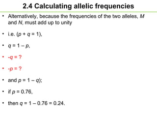
• Alternatively, because the frequencies of the two alleles, M
and N, must add up to unity
• i.e. (p + q = 1),
• q = 1 – p,
• -q = ?
• -p = ?
• and p = 1 – q);
• if p = 0.76,
• then q = 1 – 0.76 = 0.24.

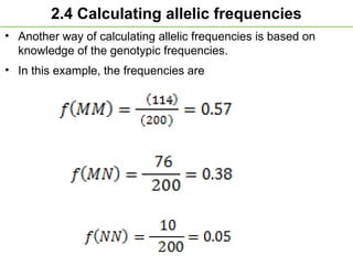
25. 2.4 Calculating allelic frequencies
• Another way of calculating allelic frequencies is based on
knowledge of the genotypic frequencies.
• In this example, the frequencies are

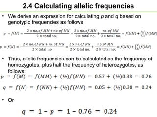
26. 2.4 Calculating allelic frequencies
• We derive an expression for calculating p and q based on
genotypic frequencies as follows
• Thus, allelic frequencies can be calculated as the frequency of
homozygotes, plus half the frequency of heterozygotes, as
follows:
• Or

27. 2.4 Calculating allelic frequencies
• These methods (counting alleles and using genotypic
frequencies) are algebraically identical and thus give identical
results.

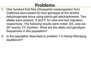
28. Problems
1. One hundred fruit flies (Drosophila melanogaster) from
California were tested for their genotype at the alcohol
dehydrogenase locus using starch-gel electrophoresis. Two
alleles were present, S and F, for slow and fast migration,
respectively. The following results were noted: SS, sixty-six;
SF, twenty; FF, fourteen. What are the allelic and genotypic
frequencies in this population?
2. Is the population described in problem 1 in Hardy-Weinberg
equilibrium?

29. 2.5 Assumptions of Hardy-Weinberg Equilibrium
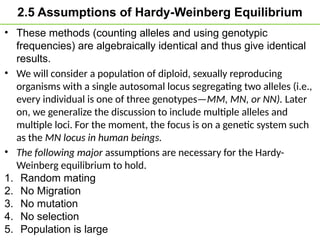
• These methods (counting alleles and using genotypic
frequencies) are algebraically identical and thus give identical
results.
• We will consider a population of diploid, sexually reproducing
organisms with a single autosomal locus segregating two alleles (i.e.,
every individual is one of three genotypes—MM, MN, or NN). Later
on, we generalize the discussion to include multiple alleles and
multiple loci. For the moment, the focus is on a genetic system such
as the MN locus in human beings.
• The following major assumptions are necessary for the Hardy-
Weinberg equilibrium to hold.
1. Random mating
2. No Migration
3. No mutation
4. No selection
5. Population is large

30. Proof of the Hardy-Weinberg equilibrium
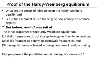
• What are the effects of inbreeding on the Hardy-Weinberg
equilibrium?
• Let us for a moment return to the gene pool concept to produce
zygotes.
 But before, remind yourself of
The three properties of the Hardy-Weinberg equilibrium
(1) allelic frequencies do not change from generation to generation,
(2) allelic frequencies determine genotypic frequencies, and
(3) the equilibrium is achieved in one generation of random mating.
Can you prove if the population remains in equilibrium or not?

31. Proof of the Hardy-Weinberg equilibrium
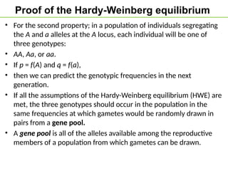
• For the second property; in a population of individuals segregating
the A and a alleles at the A locus, each individual will be one of
three genotypes:
• AA, Aa, or aa.
• If p = f(A) and q = f(a),
• then we can predict the genotypic frequencies in the next
generation.
• If all the assumptions of the Hardy-Weinberg equilibrium (HWE) are
met, the three genotypes should occur in the population in the
same frequencies at which gametes would be randomly drawn in
pairs from a gene pool.
• A gene pool is all of the alleles available among the reproductive
members of a population from which gametes can be drawn.

32. Proof of the Hardy-Weinberg equilibrium
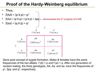
• Thus,
• f(AA) = (p X p) = p2
• f(Aa) = (p X q) + (q X p) = 2pq demonstrates the 2nd
property of H-WE
• f(aa) = (q X q) = q2
Gene pool concept of zygote formation. Males & females have the same
frequencies of the two alleles: f (A) = p and f (a) = q. After one generation of
random mating, the three genotypes, AA, Aa, and aa, have the frequencies of
p2
, 2pq, and q2
, respectively.

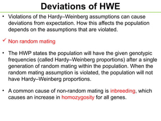
33. Deviations of HWE
• Violations of the Hardy–Weinberg assumptions can cause
deviations from expectation. How this affects the population
depends on the assumptions that are violated.
 Non random mating
• The HWP states the population will have the given genotypic
frequencies (called Hardy–Weinberg proportions) after a single
generation of random mating within the population. When the
random mating assumption is violated, the population will not
have Hardy–Weinberg proportions.
• A common cause of non-random mating is inbreeding, which
causes an increase in homozygosity for all genes.

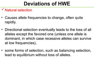
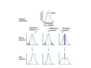
34. Deviations of HWE
Natural selection
• Causes allele frequencies to change, often quite
rapidly.
• Directional selection eventually leads to the loss of all
alleles except the favored one (unless one allele is
dominant, in which case recessive alleles can survive
at low frequencies),
• some forms of selection, such as balancing selection,
lead to equilibrium without loss of alleles.

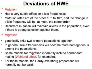
36. Deviations of HWE
 Mutation
• Has a very subtle effect on allele frequencies
• Mutation rates are of the order 10−4
to 10−8
, and the change in
allele frequency will be, at most, the same order.
• Recurrent mutation will maintain alleles in the population, even
if there is strong selection against them.
 Migration
• genetically links two or more populations together.
• In general, allele frequencies will become more homogeneous
among the populations.
• Some models for migration inherently include nonrandom
mating (Wahlund effect, for example).
• For those models, the Hardy–Weinberg proportions will
normally not be valid.

37. Deviations of HWE
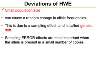
Small population size
• can cause a random change in allele frequencies.
• This is due to a sampling effect, and is called genetic
drift.
• Sampling ERROR effects are most important when
the allele is present in a small number of copies.

38. Chi-Square Test of Goodness-of-Fit to the
Hardy-Weinberg Proportions
 There are several ways to determine whether a given
population conforms to the Hardy-Weinberg equilibrium
at a particular locus.
we can determine whether the three genotypes (AA,
Aa, and aa) occur with the frequencies p2
, 2pq, and
q2
.
If they do, then the population is considered to be in
Hardy-Weinberg proportions;
if not, then the population is not considered to be in
Hardy-Weinberg proportions.

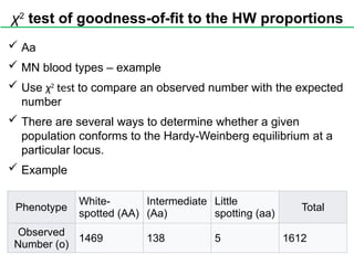
39. χ2
test of goodness-of-fit to the HW proportions
 Aa
 MN blood types – example
 Use χ2
test to compare an observed number with the expected
number
 There are several ways to determine whether a given
population conforms to the Hardy-Weinberg equilibrium at a
particular locus.
 Example
Phenotype
White-
spotted (AA)
Intermediate
(Aa)
Little
spotting (aa)
Total
Observed
Number (o)
1469 138 5 1612

40. • What were your answers??

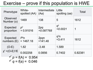
41. Exercise – prove if this population is HWE
Phenotype
White-
spotted (AA)
Intermediate
(Aa)
Little
spotting (aa)
Total
Observed
Number (o)
1469 138 5 1612
Expected
proportion
p2
= 0.91016
2pq
=0.087768
q2
=0.0021 1
Expected
numbers (E)
P2
n
= 1467.18
2pqn
=141.48
q2
n
=3.411 1612
(O-E) 1.82 -3.48 1.589
χ2
=(O-E)2
/E
0.002258 0.0856 0.7402 0.82381
 p = f(A) = 0.954
 q = f(a) = 0.046

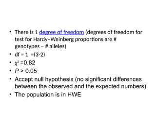
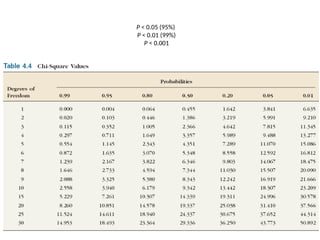
42. • There is 1 degree of freedom (degrees of freedom for
test for Hardy–Weinberg proportions are #
genotypes − # alleles)
• df = 1 =(3-2)
• χ2
=0.82
• P > 0.05
• Accept null hypothesis (no significant differences
between the observed and the expected numbers)
• The population is in HWE

43. P < 0.05 (95%)
P < 0.01 (99%)
P < 0.001

44. Exercise
• On a chicken farm, walnut-combed fowlthat
were crossed with each other produced the
followingoffspring: walnut-combed, 87; rose-
combed, 31; peacombed,30; and single-
combed, 12. What hypothesis might you have
about the control of comb shape in fowl? Do
the data support that hypothesis? (3 Marks)

45. QUIZ 1
• MM = 114
• MN = 76
• NN = 10
QUIZ 2
• MM = 152
• MN = 0
• NN = 48
• Are the data in HWE?

46. Extensions of HWE
• The HWE can be extended to include,
• among other cases, multiple alleles and multiple loci.

47. MULTIPLE ALLELISM
• When there is more than 2 alleles possible for
a given gene.
• Allows for a larger number of genetic and
phenotypic possibilities.

48. Multiple alleles
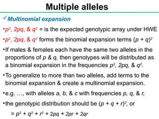
Multinomial expansion
•p2
, 2pq, & q2
= is the expected genotypic array under HWE
•p2
, 2pq, & q2
forms the binomial expansion terms (p + q)2
•If males & females each have the same two alleles in the
proportions of p & q, then genotypes will be distributed as
a binomial expansion in the frequencies p2
, 2pq, & q2
.
•To generalize to more than two alleles, add terms to the
binomial expansion & create a multinomial expansion.
•e.g. …, with alleles a, b, & c with frequencies p, q, & r,
•the genotypic distribution should be (p + q + r)2
, or
= p2
+ q2
+ r2
+ 2pq + 2pr + 2qr

49. Multiple alleles
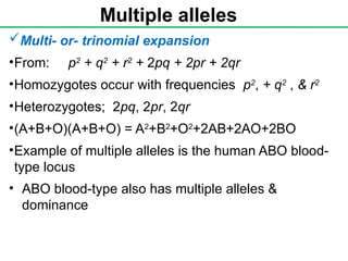
Multi- or- trinomial expansion
•From: p2
+ q2
+ r2
+ 2pq + 2pr + 2qr
•Homozygotes occur with frequencies p2
, + q2
, & r2
•Heterozygotes; 2pq, 2pr, 2qr
•(A+B+O)(A+B+O) = A2
+B2
+O2
+2AB+2AO+2BO
•Example of multiple alleles is the human ABO blood-
type locus
• ABO blood-type also has multiple alleles &
dominance

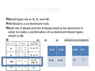
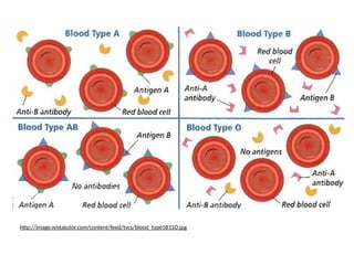
50. BLOOD TYPING
Blood types are A, B, O, and AB.
AB blood is a co-dominant trait.
Both the A blood and the B blood need to be dominant in
order to make a combination of co-dominant blood types,
which is AB.
 IA IA IA iiiiiiiiiiiiiiiiiiiiiiiiiiiiiiiii

 IB IB

 IB i
IA IB IA IB
IA IB IA IB
IA IB IB i
IA i ii
i

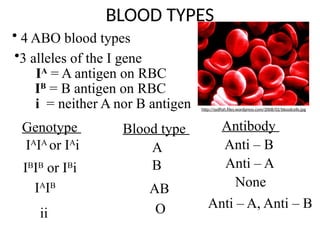
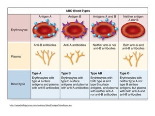
51. BLOOD TYPES
Antibody
Anti – B
Anti – A
None
Anti – A, Anti – B
• 4 ABO blood types
•3 alleles of the I gene
IA
= A antigen on RBC
IB
= B antigen on RBC
i = neither A nor B antigen
Genotype
IA
IA
or IA
i
IB
IB
or IB
i
IA
IB
ii
Blood type
A
B
AB
O
http://sydfish.files.wordpress.com/2008/02/bloodcells.jpg

52. http://www.pennmedicine.org/health_info/images/19450.jpg

53. http://duongchan.files.wordpress.com/2007/05/abobloodsystem.jpg

54. http://image.wistatutor.com/content/feed/tvcs/blood_type5B15D.jpg

55. http://www.biologycorner.com/anatomy/blood/images/bloodtypes.jpg

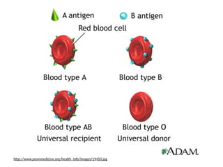
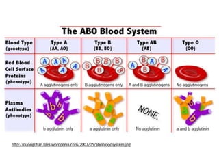
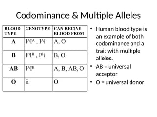
56. Codominance & Multiple Alleles
• Human blood type is
an example of both
codominance and a
trait with multiple
alleles.
• AB = universal
acceptor
• O = universal donor
BLOOD
TYPE
GENOTYPE CAN RECIVE
BLOOD FROM
A IA
IA
, IA
i A, O
B IB
IB
, IB
i B, O
AB IA
IB
A, B, AB, O
O ii O

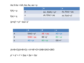
57. Aa X Aa = AA; Aa; Aa, aa = p
f(A) = p
f(a) = q
(p+q)2
= p2 +
2pq+ q2
(A+B+O)(A+B+O) = A2
+B2
+O2
+2AB+2AO+2BO
p2
+ q2
+ r2
+ 2pq + 2pr + 2qr
A a
A AA , f(AA) = p2 Aa, f(Aa) = pq
a aA, f(Aa) = pq aa, f(aa)= q2
A B o
A f(AA) = p2
AB = pq AO = pr
B f(AB) = pq BB =q2
BO = qr
o AO = pr BO = qr OO =r2

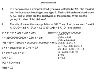
58. PRACTICE QUESTIONS
1. In a certain case a woman’s blood type was tested to be AB. She married
and her husbands blood type was type A. Their children have blood types
A, AB, and B. What are the genotypes of the parents? What are the
genotypic ratios of the children?
2. The city of Nairobi has a population of 106
. Their blood types are; B = 4.5
X 105
, O = 3.6 X 105
, A = 1.3 X 105
, AB = 6 X 104
(10 Marks)
p2
+ q2
+ r2
+ 2pq + 2pr + 2qr : f(oo) = r2
= 360000/1000000
r2
= 360000/1000000 = 0.36; r = 0.6
=(p + r)2
= (130000 + 360000)/1,000,000 = 0.49
p + r = squareroot of 0.49 = 0.7
p + 0.6 = 0.7; p = 0.1
f(A) = 0.1
f(C) = f(O) = 0.6
F(B) = 0.3
q2
+2qr = B
q2
+2qr = 0.45
q2
+2q x 0.6 =0.45
q2
+1.2q - 0.45 = 0
q2
+ 1.5q - 0.3q -0.45 = 0
q(q +1.5) – 0.3(q + 1.5) = 0
(q – 0.3) (q +1.5) = 0
q = 0.3
q = -1.5

59. • r2
= 360000/1000000 = 0.36; r = 0.6
• Blood type A = p2
+ 2pr
• p2
+ 2p x 0.6 = 0.13
• p2
+ 1.2p = 0.13
• p2
+ 1.2p – 0.13 = 0
• Then look for numbers when you multiply you get -0.13
and when you add you get 1.2
• That will be 1.3, -0.1
• p2
+ 1.3p – 0.1p-0.13 = 0
• Then factorise
• p(p +1.3) -0.1(p+1.3)=0
• (p-0.1)(p+1.3) =0
• P = 0.1, -1.3
• f(A) = 0.1
1. p2
+ q2
+ r2
+ 2pq + 2pr + 2qr

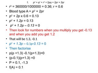
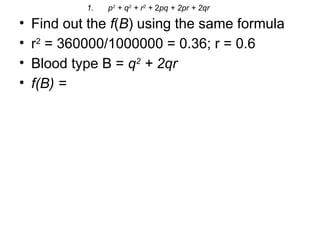
60. • Find out the f(B) using the same formula
• r2
= 360000/1000000 = 0.36; r = 0.6
• Blood type B = q2
+ 2qr
• f(B) =
1. p2
+ q2
+ r2
+ 2pq + 2pr + 2qr

62. ABO blood groups
https://www.youtube.com/watch?v=bqNi9IvakbI
• https://www.youtube.com/watch?v=Zi7DnMLUudQ
• https://www.youtube.com/watch?v=BuJThy5cSTs
• https://www.youtube.com/watch?v=w36d8DY_VfE
• https://www.youtube.com/watch?v=Rbtn8XtNefw
• https://www.youtube.com/watch?v=XoymFI0lIM8
• https://www.youtube.com/watch?v=fFt9DRysfSY

63. Multiple loci
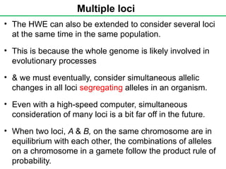
• The HWE can also be extended to consider several loci
at the same time in the same population.
• This is because the whole genome is likely involved in
evolutionary processes
• & we must eventually, consider simultaneous allelic
changes in all loci segregating alleles in an organism.
• Even with a high-speed computer, simultaneous
consideration of many loci is a bit far off in the future.
• When two loci, A & B, on the same chromosome are in
equilibrium with each other, the combinations of alleles
on a chromosome in a gamete follow the product rule of
probability.

64. Multiple loci
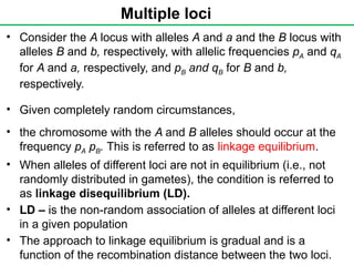
• Consider the A locus with alleles A and a and the B locus with
alleles B and b, respectively, with allelic frequencies pA and qA
for A and a, respectively, and pB and qB for B and b,
respectively.
• Given completely random circumstances,
• the chromosome with the A and B alleles should occur at the
frequency pA pB. This is referred to as linkage equilibrium.
• When alleles of different loci are not in equilibrium (i.e., not
randomly distributed in gametes), the condition is referred to
as linkage disequilibrium (LD).
• LD – is the non-random association of alleles at different loci
in a given population
• The approach to linkage equilibrium is gradual and is a
function of the recombination distance between the two loci.

65. Multiple loci
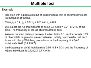
Example
• let’s start with a population out of equilibrium so that all chromosomes are
AB (70%) or ab (30%).
• Then pA = 0.7, qA = 0.3, pB = 0.7, and qB = 0.3.
• We expect the Ab chromosome to occur 0.7 X 0.3 = 0.21, or 21% of the
time. The frequency of the Ab chromosome is zero.
• Assume the map distance between the two loci is 0.1; in other words, 10%
of chromatids in gametes are recombinant. Initially, we consider that each
locus is in Hardy-Weinberg proportions, or the frequency of AB/AB
individuals 0.49 (0.7 X 0.7);
• the frequency of ab/ab individuals is 0.09 (0.3 X 0.3); and the frequency of
AB/ab individuals is 0.42 (2 X 0.7 X 0.3).

66. Multiple loci
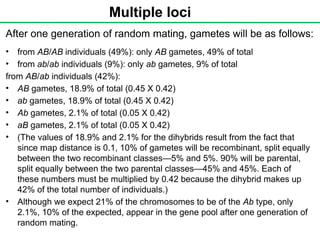
After one generation of random mating, gametes will be as follows:
• from AB/AB individuals (49%): only AB gametes, 49% of total
• from ab/ab individuals (9%): only ab gametes, 9% of total
from AB/ab individuals (42%):
• AB gametes, 18.9% of total (0.45 X 0.42)
• ab gametes, 18.9% of total (0.45 X 0.42)
• Ab gametes, 2.1% of total (0.05 X 0.42)
• aB gametes, 2.1% of total (0.05 X 0.42)
• (The values of 18.9% and 2.1% for the dihybrids result from the fact that
since map distance is 0.1, 10% of gametes will be recombinant, split equally
between the two recombinant classes—5% and 5%. 90% will be parental,
split equally between the two parental classes—45% and 45%. Each of
these numbers must be multiplied by 0.42 because the dihybrid makes up
42% of the total number of individuals.)
• Although we expect 21% of the chromosomes to be of the Ab type, only
2.1%, 10% of the expected, appear in the gene pool after one generation of
random mating.

67. Multiple loci
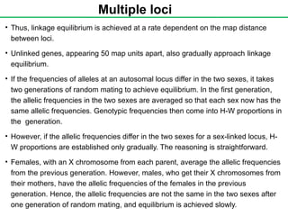
• Thus, linkage equilibrium is achieved at a rate dependent on the map distance
between loci.
• Unlinked genes, appearing 50 map units apart, also gradually approach linkage
equilibrium.
• If the frequencies of alleles at an autosomal locus differ in the two sexes, it takes
two generations of random mating to achieve equilibrium. In the first generation,
the allelic frequencies in the two sexes are averaged so that each sex now has the
same allelic frequencies. Genotypic frequencies then come into H-W proportions in
the generation.
• However, if the allelic frequencies differ in the two sexes for a sex-linked locus, H-
W proportions are established only gradually. The reasoning is straightforward.
• Females, with an X chromosome from each parent, average the allelic frequencies
from the previous generation. However, males, who get their X chromosomes from
their mothers, have the allelic frequencies of the females in the previous
generation. Hence, the allelic frequencies are not the same in the two sexes after
one generation of random mating, and equilibrium is achieved slowly.

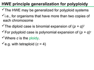
68. HWE principle generalization for polyploidy
The HWE may be generalized for polyploid systems
i.e., for organisms that have more than two copies of
each chromosome
The diploid case is binomial expansion of (p + q)2
For polyploid case is polynomial expansion of (p + q)c
Where c is the ploidy.
e.g. with tetraploid (c = 4)

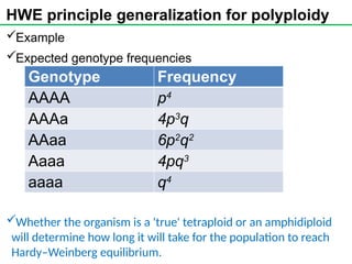
69. HWE principle generalization for polyploidy
Example
Expected genotype frequencies
Whether the organism is a 'true' tetraploid or an amphidiploid
will determine how long it will take for the population to reach
Hardy–Weinberg equilibrium.
Genotype Frequency
AAAA p4
AAAa 4p3
q
AAaa 6p2
q2
Aaaa 4pq3
aaaa q4

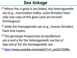
70. Sex linkage
Where the A gene is sex linked, the heterogametic
sex (e.g., mammalian males; avian females) have
only one copy of the gene (and are termed
hemizygous),
while the homogametic sex (e.g., human females)
have two copies.
The genotype frequencies at equilibrium
are p and q for the heterogametic sex but p2
,
2pq and q2
for the homogametic sex.
https://www.youtube.com/watch?v=l_amQ12X98o