Running head: Statistics 2 Statistics Statistics Name: Course: Instructor: Institution: Date of Submission: Assignment #4: Model Diagnostics A fundamental requirement in the classical linear regression is that the regression error term must be normally distributed with zero mean and constant variance (Greene, 2008). The normality tests results are presented below. All the plots have values greater than the threshold probability value of 0.05 thus the null hypothesis of normality of the regression residuals could not be rejected at 5 per cent significance level. Conclusion is thus made that the regression residuals from the estimated equations followed a normal distribution. Since any linear function of normally distributed variables is considered to be normally distributed, normal distribution of the residuals had the implication that the coefficients of the estimates were also themselves normally distributed (Gujarati, 2008). The residual plot is shown below: From the residual plot it can be seen that all the residuals fall within the standard error bands thus confirming that the model is stable and can thus be used for forecasting. References Greene, W. (2008). Econometric analysis, 6th ed. . New Jersey: Pearson-Prentice Hall. Gujarati, D. (2004). Basic econometrics 4th ed. . New York: McGraw Hill Companies. Normal Probability Plot 2.6315789473684208 7.8947368421052602 13.15789473684211 18.421052631578942 23.684210526315791 28.947368421052641 34.21052631578948 39.473684210526301 44.73684210526315 50 55.26315789 4736857 60.526315789473699 65.789473684210563 71.052631578947384 76.315789473684163 81.578947368420984 86.842105263157904 92.105263157894726 97.368421052631547 10.7 11.3 11.8 11.9 12 12 12 12.4 12.5 12.6 13.1 13.2 13.4 13.5 13.5 14.2 14.5 14.5 14.6 Sample Percentile MedianSchoolYears Age Residual Plot 60 30 62 44 0 30 62 68 46 56 36 28 0 0 34 26 52 50 44 0.50878516451792 1.7144464705013149 -0.42159945482941003 0.54117037792769895 0.71299080887547295 1.269413932725179 0.26951686627728799 0.22131431339594501 -0.13472012994437299 0.22075061567252199 -1.3199768562363781 -0.18681496091028299 0.380020030213299 -1.451131014273024 -0.56052688701790399 -0.116260966970037 -0.67291294283960901 -0.49015761805784802 -0.48430774902780499 Age Residuals RUNNING HEADER: WEEK 3 ASSIGNMENT 4 1 WEEK 3 ASSIGNMENT 4 13 Week 3 Assignment 4 Introduction In this project I selected six variables from the ' SampleDataSet.xlsx'. Among these six variables three of them were continuous and the reaming three were discrete variables. The continuous variables selected for this study are Age, WealthScore and MedianSchoolYears. The discrete variables selected for this study are NumberOfChildren, MailResponder and NumberOfCars. Analysis Age The age is a continuous variable which takes only positive values even though we usually consider the integer part of it. The descriptive statistics summary of the age variable .

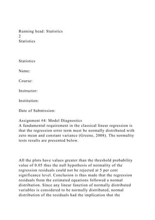
1. Running head: Statistics
2
Statistics
Statistics
Name:
Course:
Instructor:
Institution:
Date of Submission:
Assignment #4: Model Diagnostics
A fundamental requirement in the classical linear regression is
that the regression error term must be normally distributed with
zero mean and constant variance (Greene, 2008). The normality
tests results are presented below.
All the plots have values greater than the threshold probability
value of 0.05 thus the null hypothesis of normality of the
regression residuals could not be rejected at 5 per cent
significance level. Conclusion is thus made that the regression
residuals from the estimated equations followed a normal
distribution. Since any linear function of normally distributed
variables is considered to be normally distributed, normal
distribution of the residuals had the implication that the

2. coefficients of the estimates were also themselves normally
distributed (Gujarati, 2008).
The residual plot is shown below:
From the residual plot it can be seen that all the residuals fall
within the standard error bands thus confirming that the model
is stable and can thus be used for forecasting.
References
Greene, W. (2008). Econometric analysis, 6th ed. . New Jersey:
Pearson-Prentice Hall.
Gujarati, D. (2004). Basic econometrics 4th ed. . New York:
McGraw Hill Companies.
Normal Probability Plot
2.6315789473684208 7.8947368421052602
13.15789473684211 18.421052631578942
23.684210526315791 28.947368421052641
34.21052631578948 39.473684210526301
44.73684210526315 50 55.26315789 4736857
60.526315789473699 65.789473684210563
71.052631578947384 76.315789473684163
81.578947368420984 86.842105263157904
92.105263157894726 97.368421052631547 10.7
11.3 11.8 11.9 12 12 12 12.4 12.5 12.6 13.1 13.2
13.4 13.5 13.5 14.2 14.5 14.5 14.6
Sample Percentile
MedianSchoolYears
Age Residual Plot
60 30 62 44 0 30 62 68 46 56 36 28 0
0 34 26 52 50 44 0.50878516451792
1.7144464705013149 -0.42159945482941003
0.54117037792769895 0.71299080887547295
1.269413932725179 0.26951686627728799

3. 0.22131431339594501 -0.13472012994437299
0.22075061567252199 -1.3199768562363781 -
0.18681496091028299 0.380020030213299 -
1.451131014273024 -0.56052688701790399 -
0.116260966970037 -0.67291294283960901 -
0.49015761805784802 -0.48430774902780499
Age
Residuals
RUNNING HEADER: WEEK 3 ASSIGNMENT 4 1
WEEK 3 ASSIGNMENT 4 13
Week 3 Assignment 4

4. Introduction
In this project I selected six variables from the '
SampleDataSet.xlsx'. Among these six variables three of them
were continuous and the reaming three were discrete variables.
The continuous variables selected for this study are Age,
WealthScore and MedianSchoolYears. The discrete variables
selected for this study are NumberOfChildren, MailResponder
and NumberOfCars.
Analysis
Age
The age is a continuous variable which takes only positive
values even though we usually consider the integer part of it.
The descriptive statistics summary of the age variable are
shown below.
Table -1: Descriptive statistics of Age
Age
Mean
46.202
Median
48
Mode
0
Standard Deviation
20.85197
Sample Variance
434.8046
Kurtosis
0.249096
Skewness
-0.67306
Range
96
Minimum
0

5. Maximum
96
Sum
92404
Count
2000
Table-1, shows that the data consists of the ages of 2000 people.
The mean age is 46.202 years, median age is 48, but the mode is
0. The largest age is 96 with variability measured by standard
deviation is 20.85.
Graph-1: Distribution of Age
The age distribution using histogram is shown is Graph-1.
Bearing a clustering at 0, the distribution of age is
approximately symmetric.
Wealth Score
Table -2: Descriptive statistics of WealthScore
WealthScore
Mean
301.8376
Median
299.01
Mode
490.46
Standard Deviation
94.35198
Sample Variance

6. 8902.296
Kurtosis
-0.66676
Skewness
0.124734
Range
390.46
Minimum
100
Maximum
490.46
Count
2000
Table-2, shows that the data consists of the wealth scores of
2000 samples. The mean score is 301.84, median age is 299.01
and the mode is 490.46. The largest age is 490.46 with
variability measured by standard deviation is 94.35.
Graph-2: Histogram of wealth score
The histogram of the wealth scores in Graph -2 shows that the
distribution is approximately symmetric and bell shape.
Median School years
Table -3: Descriptive statistics of MedianSchoolYears
MedianSchoolYears
Mean
13.26322
Median
13.2
Mode
12

7. Standard Deviation
1.424966
Sample Variance
2.030528
Kurtosis
-0.21916
Skewness
0.303654
Range
12.4
Minimum
5.7
Maximum
18.1
Count
1903
From Table-3 we can see that the sample consists of the median
school years of 1903 people. The mean of the variable is 13.26
years, median age is 13.2 and the mode is 12 years. The
maximum years is 18.1 with variability measured by standard
deviation is 1.42 years.
Graph-3: Histogram of school years
The histogram of the median school years in Graph -3 shows
that, the distribution is approximately positively skewed.
Number of Children
Table -4: Descriptive statistics of the number of children
NumberOfChildren
Mean
0.586
Median

8. 0
Mode
0
Standard Deviation
1.020355
Sample Variance
1.041125
Kurtosis
3.045176
Skewness
1.876443
Range
6
Minimum
0
Maximum
6
Sum
1172
Count
2000
The descriptive statistics of the number of children shows that
the average number of children is 0.586 with majority having no
children. Further the distribution of the number of children is
positively skewed.
Table -4: Frequency table representing the number of children
NumberOfChildren
Frequency
0
1355
1
323
2

9. 174
3
99
4
42
5
6
6
1
Graph-4: Frequency distribution of the number of children
Graph-5: Pie chart representing the number of children
Mail Responder
The mode of the variable mail responder is 2
Table 5: Frequency of the mail responder
Mail responder
Frequency
0
447
1
515
2
1038

10. Graph-6: Pie chart representing the mail responder
It shows that the mode of the variable mail responder is 2.
Number of cars
Table 6: Descriptive statistics for the number of cars
NumberOfCars
Mean
1.0313
Median
1
Mode
1
Standard Deviation
1.0557
Sample Variance
1.1146
Kurtosis
6.0731
Skewness
1.72
Range
9
Minimum
0

11. Maximum
9
Sum
956
Count
927
Hypothesis tests
The first hypothesis tested in this study is regarding the mean
age. The null hypothesis H0 was that the mean age of the
population is 50. Alternative hypothesis H1 was that the mean
age of the population is less than 50. 5% level of significance is
used to test the hypothesis. The null hypothesis was rejected (t
=-8.145, df= 1999, p value <0.000) at 5% level. Therefore, we
conclude that there is enough evidence to support the claim that
the mean age is less than 50.
Table 7: Test for the mean age
Age
hypo. Value
Mean
46.202
50
Variance
434.8046
0
Observations
2000
2000
Pearson Correlation
#DIV/0!
Hypothesized Mean Difference

12. 0
df
1999
t Stat
-8.1456
P(T<=t) one-tail
3.29E-16
t Critical one-tail
1.645616
P(T<=t) two-tail
6.57E-16
t Critical two-tail
1.961151
Now the hypothesis tested in this study is regarding the mean
wealth score. The null hypothesis H0 was that the mean wealth
score of the population is 300. Alternative hypothesis H1 was
that the mean wealth score of the population is not equal to 300.
The null hypothesis was not able to rejected (t 0.871003, df=
1999, p value = 0.389) at 5% level. Therefore, we conclude that
there is not enough evidence to support the claim that the mean
wealth score is different from 300. Details are given in Table -
8
Table 8: Test for the mean wealth score
WealthScore
Null wealth

13. Mean
301.8376
300
Variance
8902.296
0
Observations
2000
2000
Pearson Correlation
#DIV/0!
Hypothesized Mean Difference
0
df
1999
t Stat
0.871003
P(T<=t) one-tail
0.191929
t Critical one-tail
1.645616
P(T<=t) two-tail
0.383857
t Critical two-tail
1.961151
The third hypothesis tested in this study is regarding the mean
value of the median school years. The null hypothesis H0 was

14. that the mean school year of the population is 12 years.
Alternative hypothesis H1 was that the mean school year of the
population is greater than 12 years. The null hypothesis was
rejected (t =38.672, df= 1902, p value <0.000) at 5% level.
Therefore, we conclude that there is enough evidence to support
the claim that the mean of teh median school years is greater
than 12.
Table 9: Test for the mean school years
MedianSchoolYears
Null schoolyears
Mean
13.26322
12
Variance
2.030528
0
Observations
1903
1903
Pearson Correlation
#DIV/0!
Hypothesized Mean Difference
0

15. df
1902
t Stat
38.67163
P(T<=t) one-tail
3.4E-242
t Critical one-tail
1.645655
P(T<=t) two-tail
6.9E-242
t Critical two-tail
1.961212
Now a chi-square test is conducted to test the independence of
the number of children and the number of Cars. The null
hypothesis H0 was the number of children and the number of
cars is independent. The alternative hypothesis H1 is that the
number of children and the number of cars is dependent
Table 10: Contingency table
zero
one
two
three
four
Five
Six above
Total
zero

16. 940
274
94
32
8
3
1
1352
one
223
51
30
16
1
1
1
323
two
113
35
15
6
2
0
1
172
three
75
14
6
2
1

17. 0
1
99
four
24
13
4
0
0
0
1
42
Five
5
1
0
0
0
0
0
6
Six
1
0
0
0
0
0
0
1
Total
1381

18. 388
149
56
12
4
5
1995
Table 11: Hypothesis test
35.99
chi-square
36
df
.4691
p-value
The null hypothesis was not to reject ( = 35.99, df=36, p value
<0.4961 ) at 5% level. There is not enough evidence that the
number of children is independent of the vehicles.
Limitations of the study
There were a number of missing observations in the variable,
number of cars. The t test assumes that the distribution of the
population is normal. But we have not conducted the study for
normality of the populations.

19. References
Doane and Seward (2010), Applied Statistics in Business and
Economics: the McGraw Hills Ltd.
Linda, Marchal, and Wathen (2008), Statistical Techniques in
Business & Economics, 13th
edition. New York, NY: McGraw Hill.
Number of Children
NumberOfChildren 0 1 2 3 4 5 6
Frequency 1355 323 174 99 42 6 1
Number of childrens
zero one two threefour five six 1355 323 174 99 42 6
1 Frequency zero one two 447 515 1038
Histogram of Age
Frequency 0 5 10 15 20 25 30 35 40 45
50 55 60 65 70 75 80 85 90 95 100
More 202 0 0 0 1 29 128 111 206
173 265 171 240 158 118 65 89 24 15 2 3
0
Age
Frequency
Distribution of WealthScore
Frequency 0 25 50 75 100 125 150 175 200

20. 225 250 275 300 325 350 375 400 425 450 475
500 More 0 0 0 0 9 26 64 82
118 167 183 172 192 179 174 176 138 98 64 58
100 0
WealthScore
Frequency
Histogram of MedianSchoolYears
Frequency 5 6 7 8 9 10 11 12 13 14
15 16 17 18 More 0 1 0 0 0 1
42 405 452 447 298 204 45 7 1
MedianSchoolYears
Frequency
Sheet1HouseholdIDCityStateMSACodeGenderAgeWealthScore
NumberOfChildrenMailResponderMedianSchoolYearsNumberO
fCarsAB100794446ManchesterCTF60141.120112AgeWealthSco
reMedianSchoolYearsBL103110217AnkenyIAM30246.380014.5
Mean46.202Mean301.83762Mean13.2632159748AL100297826L
ake
TappsWAM62375.330213.5Median48Median299.01Median13.2
AK103361183Grand
RapidsMIM44333.884213.42Mode0Mode490.46Mode12AP1008
08185O FallonMOF0336.181214.52Standard
Deviation20.8519686912Standard
Deviation94.3519774088Standard
Deviation1.4249661236AL102281729KnoxvilleTNM30323.682
214.61Sample Variance434.8045982991Sample
Variance8902.2956409562Sample
Variance2.0305284533AA100557115CambridgeMN5120F62332
.890213.51Kurtosis0.2490959725Kurtosis-
0.6667619166Kurtosis-
0.2191568703AU102418311StoughtonMA1120M68384.210114.
2Skewness-
0.6730571911Skewness0.1247339266Skewness0.3036538561BS
102737313RaymondNH4160F46295.392112.60Range96Range39
0.46Range12.4BQ103379666North

21. MankatoMNM56274.670213.12Minimum0Minimum100Minimu
m5.7AX102690269Los
AngelesCA4480M36363.492212.4Maximum96Maximum490.46
Maximum18.1AJ102079864AzleTX2800F28190.131011.8Count
2000Count2000Count1903BG101542955EasthamptonMA8000M
0217.760013.2AM100685288Las
VegasNV4120F0270.390012BF101795019RossvilleGA1560F34
102.30010.7AS101518382Lehigh
AcresFL2700M26174.670011.91NumberOfChildrenBT10258114
6West
ColumbiaSC1760M52376.972212.5Mean0.586AE102386836Wa
rner
RobinsGA4680F50180.261011.3Median0BT101916705AkronO
H80F44244.0812120Mode0AF101535688JohnstonRI6480M4835
7.571212.2Standard
Deviation1.0203551158BT100905543MineolaTXM60178.62321
1.50Sample Variance1.0411245623AR100318955Grants
PassORF82284.210211.92Kurtosis3.0451756334AH100794933S
alemORF38261.513012.30Skewness1.87644329AB101731499So
mers
PointNJ560F66234.210012.3Range6BS100678069PetalumaCA7
500M66490.460214.6Minimum0BB100821672MoosupCTF4631
0.534212.1Maximum6BA102835475CovingtonGA520M66299.3
41211.5Sum1172AK100931054DillonSCF54190.131011Count2
000AP102795843FlemingtonMOF46191.120211.52AY10259939
6CerritosCA4480M64490.460215.3BH102034931ColumbiaSC1
760F52203.290015.2BT102671792WalhallaSCM68151.320111.
5AP102934858EdenNY1280M38285.862113.51NumberOfChildr
enFrequencyAR102810155CorvallisMTF64274.670213.1001355
AG102694587SalinaKSF76186.840213.31323AA100276439Cre
stviewFL2750F58229.28011212174AZ104193154BaltimoreMD7
20M38369.7412399AL101833829Chicago
HtsIL1600F0127.960211.4442AX100815576CovingtonVAF382
47.72111.956BT100779542Holly Lake
RaTXM70136.840112.8161AT103418941Crp
ChristiTX1880M88325.990214.12AF102360978Queens

22. VlgNY5600M58349.340212.31AH105381822DallasOR7080F02
06.2500AT103049290LititzPA4000F52200.660010.8BM102055
805LanettALM34178.950211.42AN103221326MishawakaIN780
0M48332.241213.7BK102944161WestfieldNY3610M46283.552
111.91BE102692940Walnut
CreekCA5775M46376.641015.3AM107675543Mount
AiryNCM46144.0802AD102631952W
LafayetteOHF50245.070011.91BL103145929BonoAR3700M401
53.290111.5BL101632308LavoniaGAF0191.450011.5BF102458
607MoorefieldWVF441000111.23NumberOfCarsBA102412106
El DoradoARF44232.570011.9Mean1.0313AH107223164San
AntonioTX7240F32195.7202Median1AK100357946CorinthNY1
60M44234.870211.20Mode1AV101609047Rock
SpringsWYM46307.241212.40Standard
Deviation1.0557AF102538917Oro
ValleyAZF78312.170214.32Sample
Variance1.1146AM100514226Las
VegasNV4120F54361.510114.2Kurtosis6.0731AV102445978Da
llasTX1920M48479.932215.70Skewness1.7200AA100769642No
rthfieldMNM52364.471213.70Range9AF102614966Land O
LakesFL8280F48321.380213.71Minimum0AD101964085Ft
WashingtonMD8840F50479.931116.41Maximum9AZ101219912
BaltimoreMD720F0160.20211.30Sum956BP103770881Springda
leAR2580F82261.180213.2Count927AW101489070Cedar
LakeIN2960F64287.51112.2AC103036404MiltonPAF30186.840
211.8BF102101576WellingtonKSF0195.070012.4AA100672436
HastingsMN5120F38397.374113.10AG102902028Mount
GileadNCF54158.550011.1AC103075969WestlandMI2160M682
93.420112.10AA103111338RayneLA3880M46235.861111.12BN
100801354Virginia
BchVA5720M58304.930014BC102673603SheboyganWI7620F2
4155.260012.20BA100278000DecaturGA520F56239.140213.4B
N102583295Virginia
BchVA5720F50259.870213.1BT101169040WilliamstonSC3160
M40260.860213.2AE102603986MorgantonNC3290M32256.251
013.2BH102376470IrwinPA6280M48293.423213.8AL10309146

23. 7ShorewoodILM36384.872213.8AG102393477JacksonvilleILF2
4113.160112.4AQ101338258CincinnatiOH1640M0244.410213.8
0BS102679582SaginawMI6960F70285.5302131AR100939542M
enashaWI460F50215.790212.90AY102590518OrangeburgNY56
00M58367.430213.81BL108525681KodakTN3840F5827502BC1
02968773FranklinTN5360F36381.254215.20BN102285416Woo
dbridgeVA8840M76335.20212.5BL103004438BufordGA520F36
376.641013.4BR102037394Rochester
HilMI2160F30488.820216.2AM100638206PrincetonWVF0113.8
20210.30BK103109381Kansas
CityKS3760F72205.920211.3BN101853156OceansideNY5380M
64335.860214.11AN103304793WilmingtonMA1120F52362.170
213.1BL102831397FindlayOHM58225.330112.32BC101775331
HilliardFL3600M62242.110211.41BQ100473323CoatesvillePA6
160F48279.610213.5AH102858283PittsburghPA6280F70263.49
0213.9AT103256521PlainfieldIN3480M68302.30212.3BH10242
4743OrangeCA5945F52440.130213.6BN102078493GambrillsM
D720M56490.460015.10BM102213200RumfordMEF0193.42101
1.52AZ101505233ParkvilleMD720M42331.252211.80AR10225
4233Gt
BarringtonMA6320M62391.780213.5BP101620826Fayetteville
AR2580M38267.430012.5BM102264474WayneMEF44294.4102
13.50AN100885808NashvilleTN5360F40314.82113.70BT10333
3242AndersonSC3160M74262.830212.7BD101332949Laguna
HillsCA5945M62490.460215.9AZ101489427UplandCA6780F78
460.530215.2AY100792419KyleTX640F34267.430211.72AT10
1706823TownsendDE9160M72289.80111.80AE100055101Staff
ordTX3360U0247.040014.9AX102546238LeonardND2520F602
80.260213.20BM102830415Jacksons
GapALM40403.950112.30AH102784743LovettsvilleVA8840M4
4431.583114AT101126160FlandersNJ5640M32383.221114.4AE
101634892GriffinGA520M48341.122211.2AM100118934IvinsU
TU76441.780214.51BD101822200Palm Beach
GaFL8960F34205.9202120BinAP103442556CantonMOM42150.
330111.815BG103083025BordentownNJ6160M72282.890112.8
6BJ101093115LoganUTM0196.38001417BP103121276Cumberl

24. andWIF0314.470212.108AW105540056ElizabethtonTN3660F56
261.18009BR108184235AustinTX640F38300.330210BE106184
189SacramentoCA6920M58490.461211AG102489643TacomaW
A8200M44293.75011412AM102628705BatesvilleARM52251.32
0212.513AY103342033ChesterfieldVA6760M52401.641213.914
AF102547568Mt
PleasantMIM58245.390212.8015BJ100039888CarlsbadCA7320
M26323.68001516AA100283829EugeneOR2400M76279.612113
017BB101099406AugustaGA600M26211.511012.218AH102626
809PittsburghPA6280F28180.590114.7AE102833431LancasterC
A4480F76376.641113.5AL102814168El
PasoTX2320F38267.7642150BG102800831KenoshaWI3800M44
385.22212.42AA100869631StacyMN5120M0222.040012.3BP90
1623289Beale
AfbCA9340F40341.1222BL103016957DavisonMI2640F66232.8
90113.31AB103131248BellevilleIL7040F32359.543213.9BF102
401293EdinboroPA2360F0220.070214.6AH102416109Franklin
NCF70207.570112.2AD100369201DenverCO2080M36346.3811
15.20BH101537916ScottsvilleKYF32164.143011.62AH1007483
47PennsvilleNJ6160M34284.211011.7BL101079354Otter
LakeMI2160M62199.340011.81BR102536246AvonOH1680M78
405.5902141BD101236205LebanonNHF38308.220113.4AJ1015
75308FayettevilleNC2560M76196.380211.3BM102744192San
DiegoCA7320M78364.80212.2BD102386771NewportNHM6024
4.742211.10AS102241692DetroitMI2160F52231.911111.81AY1
03163043ChesapeakeVA5720F56329.610213.6BS102298773Sag
inawMI6960F58302.630213.40AF101459659Weeki
WacheeFL8280M64224.010211.82AR101670935DaltonMA6320
F30223.680213.6AG101952567ArabALF0123.360111.40AX102
047016ChicagoIL1600M52390.130213.6AJ101007612Columbus
OH1840F0131.250011.70AX102967928ChicagoIL1600M34281.
911212.2AB101635695BellevilleIL7040F34346.050213.3AQ10
1961304ValenciaCA4480M62464.470215.4BT101534116Albion
MI3720F88159.5400121AF102774154MinneapolisMN5120M48
366.452013.1BJ100899438RochesterNY6840F48268.091012.60
AE105817951ProspectCT8880M64362.502AL103225652Lockpo

25. rtIL1600M78374.340213.3AH102617735VoorheesNJ6160F0421
.712215.2AQ101804329WarwickRI6480F40468.422216.1BG10
1316598AgawamMA8000F62296.050112.7AS101530489Tempe
AZ6200F0216.780014.20AF100344417Crescent
CityFLM66141.120211.50AL100238310IndianapolisIN3480M3
0168.090012.3AA100076969LindonUT6520M38287.170014.10
AE102881809Battle
CreekMI3720M48328.622212.60AK102854739ColumbiaCT328
0F62344.740214BB102183520BrentwoodNY5380F0196.380011
.4BK102377431ZionIL1600F44213.820011.7BP102089869Sprin
g
ValleyOH2000F34188.160111.80AB103665743TariffvilleCT32
80F62244.740114.6AR100186213LagrangeINF46300.331211.1
AE102784530SealyTXM42266.120212.30BP103421914LindenN
J5640F60334.210211.6AR100173086Wild
RoseWIM78217.110211.80BL101197088Walnut
RidgeARF58169.410111.2BH102717235Smiths
GroveKYM42185.20211.20BJ102224295MoultrieGAF0163.820
112.3AX101240626ChicagoIL1600M64304.610213.6AU101810
327Bonita
SpgsFL2700M46262.830112.10AK103624110LongsSC5330M78
269.741111.8AJ101838415ClintonNCF52179.610112.2BP10172
1489NixaMO7920F282502213.13BH100086916Garden
GroveCA5945F0160.530111.8AQ102387302SheltonCT1160M68
418.090215.1AK102982651WyomingMIM62277.960213.81AU1
01808169BridgewaterNJ5015M66490.460015.7AT102000802Wi
lliamsburgMIF44308.220013.61AC102746789Sun City
WestAZ6200M80287.830213.31BB102298149RonkonkomaNY5
380M64382.8902122BK102612042MantecaCA8120F56229.930
012.1AK100645988OmahaNE5920F26185.20013.3AD10321718
2Rapid
CitySD6660M72253.290113.51AL102872255GeorgetownKY428
0F58324.340112.41BJ103249435LoganUTF50285.24215.32BA1
06413666LancasterPA4000M30189.1400AT101134198Greenwo
odIN3480F50350.330213.8BG102425554Hyde
ParkNY2281M60352.30213.92AN100569349NashvilleTN5360

26. M48454.931215.50AK102165325AlbemarleNCM0124.670010.7
AQ100374628PorterTX3360F64212.830011.53BK108030307He
metCA6780F38300.9900AA100486805Gulf
BreezeFL6080F0242.110014.2AX103167932ChicagoIL1600M8
6308.880211.5BF103014037PontiacILM44324.010212.2AQ102
833883San
FranciscoCA7360M40437.52015.6BR100290936Wolverine
LakMI2160F38343.420213.50AX103054028Niagara
FallsNY1280M52231.251211.11BF100429467East
FalmouthMA740F92359.540213.2BG102632593WaukeshaWI50
80M52178.290011.9BF103075805TuliaTXM38170.723110.70B
D102236263EscanabaMIM44320.392213.31BT102525361Ridge
NY5380M80416.121212.41AM101926261HendersonKY2440M5
2265.460012.33AA102616380MartinsburgWVF42347.373112.6
2AM101250945FoleyAL5160M44285.200133AH102413529Mul
lica
HillNJ6160M40463.821214.8BR101641835AustinTX640M0363.
490016.30AD103079508Ft
LauderdaleFL2680F40210.5300121AK103198584WinslowAZM
28157.572012.8AM102550045Las
VegasNV4120M58350.660213.2AF102595499MinneapolisMN5
120F28223.680113.13BH100509882South
BeloitIL6880M0298.680013.5AW100512707Fort
CollinsCO2670F0369.080015.41BN102423209AmaLA5560M64
275.333211.60BR100963896Avon
LakeOH1680U0222.70012.90AA101515468New
IberiaLAF52258.881111.41AC102762188OldtownMD1900M462
50.993211.11AB103572357HomosassaFLF90148.680111.61BG
103166396Eau
ClaireWI2290M68290.790112.71BC100514911BedfordVA4640
M38243.420211.3BE102654349Union
CityCA5775F44475.662213.2BK100096740HemetCA6780M401
09.540111.4AW102778378KingsportTN3660M68396.050015.1
AH100320352BlanchardOK5880F50229.280012.6AE103173889
Battle
CreekMI3720M72293.090214.11AE101819894ClintonMS3560F

27. 60392.110215.11AY103228031JacksonvilleNC3605M48298.682
213.5AL101958531Harker
HtsTX3810F28212.831214.22AJ103037795FayettevilleNC2560
M62273.681213.1BT103043047KokomoIN3850F58285.530213.
1AM101119098Cherokee
VlgARM58214.470112.9AK101711939RenoNV6720U0229.930
212.3BC102330827LebanonTN5360M44344.740212.61BF10124
9600AylettVAF42313.163111.7AZ101593707RockvilleMD8840
M66387.512162AB100095626ByhaliaMSF0131.250011.21AY10
2523100Wind GapPA240M60283.220011.5BP100753167Pearl
RiverLA5560F62237.501111AA100898578Berkeley
SpgsWVF52257.240111.40BJ100816904EscondidoCA7320M64
454.930113AZ101854514Sparrows
PtMD720F22219.080011.10AQ102871560CincinnatiOH1640F3
8311.510215.31AZ101367011Curtis
BayMD720M60320.720213.30AE102176682MilledgevilleGAF0
274.340213.4BG102236389WrightstownNJ6160F62331.910012.
8BJ103066235WoodlandCA9270M46372.043213.2BJ101882340
New
RichmondOH1640M38203.952011.72AD102704509GaryIN2960
F0254.610213.8BC100837065Madison
HtsVA4640F60282.240211.8BP100298128WinlockWAM56314.
140012.3AS102359690TempeAZ6200M76387.50215.61AC9015
61413AtlantaGA520M46254.9312BF102559244Mc
CookNEM54261.510213.45AJ102978893HilliardOH1840M7031
3.160214.50AJ901252029ColumbusOH1840F62398.6802AL101
967832Calumet
CityIL1600M72265.130112.5AQ100138205Thousand
OaksCA8735F0398.680015AQ107116447CincinnatiOH1640F26
187.1732BH102492663HatboroPA6160M72337.830214AL1076
10404Ocean
GroveNJ5190M62323.3602AP103277930KirklandWA7600F282
83.880113.5AE102717921Sugar
GroveNCM64231.910111.5AL102845858FresnoCA2840F52234.
870014.8AF102586768Ormond
BeachFL2020F54318.090114.51BQ100722073BatesvilleINM24

28. 248.360012.1AK102418266AnnandaleVA8840M48314.80013.3
AL103545539IndianapolisIN3480F62245.390213.3AQ10046531
8AnsoniaCT1160F44375.330212.4BQ103731078HopkinsMI300
0F48279.280111.70AC100622267Allen
ParkMI2160M52237.50113.12AG100061851MedfordWIM0139.
80011.41AA102788280NilesIL1600F18390.793012.2BC102776
660Chula VistaCA7320M48441.780213.7BQ102074941Liberty
TwpOH3200F78234.540212.11AW101225515FairportNY6840M
26252.301152AC102793279Fresh
MeadowsNY5600M58447.040115.11AU101013965ArcadiaFLM
281000011.20AF102870850Salt Lake
CtyUT7160F54333.881112.61AG102797459East
HartfordCT3280M42330.920212.7AZ101647193BaltimoreMD72
0F64447.040116.31AJ102536393AledoTX2800M74283.550214.
23BG101636507Pleasant
PrWI3800F52325.330213.63AW102419361WhitingIN2960F422
59.872013AS102133636Hoffman
EstatILM58318.0902BS102705891MuskegonMI3000M68271.38
0012.91AH101924483HammontonNJ560F38320.070111.8AH10
2839000PittsburghPA6280F60258.550213.8AC102786518South
LyonMI2160M60362.50213.30AA100811729OremUT6520M443
42.110113.60BH100492074Flat
RockALF60241.781210.72BJ101568126El
CajonCA7320F48381.250112.9BB101345292MurphyNCF56193.
420011.6BG102783855S
MilwaukeeWI5080F44183.220012.1AA102691471PhiladelphiaP
A6160F52157.240011.1BL100402626Oklahoma
CityOK5880F78158.220111.8BK103012676MurrietaCA6780M5
8480.920213.9AM102727671Valley
VlgCA4480F40316.120015.2AD102767455Haltom
CityTX2800M36337.1721142AW102715945PortageIN2960M72
297.370211.9AN103662561LakevilleIN7800M40343.424212.6B
L100804875HollyMI2160M0402.960013.4AZ101827814Baltim
oreMD720F54247.70211.2AD101005176DenverCO2080M66401
.970015.41AB102360070LongviewWAM56315.130013.3BQ101
920238GreensburgKYF34162.170110.91AA100174570Clearfiel

29. dUT7160M28195.720112.42AT103102616BristolVA3660F3426
3.492213BC102365965SolonOH1680F52447.0411151AM10115
0337TalmoonMNM30189.140012.42AE101458528BeasleyTX33
60F32195.070011.31AE103430082DecaturMI3720F32174.0112
11.60BC103764295MonroeVA4640F82220.720211.6AA100305
097EugeneOR2400F40316.121013AQ102741093MiddletownRIF
64310.531214.9AJ101813055LittletonCO2080F52446.050215.7
1AB101468969ColumbusGA1800F44329.283212.9BQ10378255
4DillsboroIN1640F84290.460011.6AR106386307Las
CrucesNM4100F34194.7420BP102948978Jersey
CityNJ3640M50186.180012.3BS100027091AndersonIN3480F32
143.751011.9AY100109218MoultonAL2030M34175.9910121A
Q102485278CincinnatiOH1640M68323.030214.61BD10208655
7Laguna HillsCA5945M40490.463216.1AN103231111Royal
OakMI2160F76227.6301122AB100688090LudlowKY1640F601
82.240211.41AF100963351Palm
CoastFL2020M72341.450212.92AD100023155EvansvilleIN244
0M36123.360012.1BJ103688950CordovaALF56110.20111.3BM
103075161Saint LouisMO7040F0153.2900111AQ101462218N
KingstownRI6480M86275.990113.4AP103680786WestbrookME
6400F0209.2101131AT102176535CambridgeOHF38172.70011.
80BT103153958BeltonSC3160F44207.571011.5AD103087981B
owieMD8840F60384.2101141BA901388844EriePA2360F70220.
7202AH100004243MantuaNJ6160F70185.530211.9BP10329867
7BurlingtonVTF68290.791112.6AR100174580LagrangeINF423
00.661211.6BP103765050PassaicNJ875F72259.870211.8AF102
417807Flagler
BeachFL2020F62213.490213.82AJ101010852Highland
ParkNJ5015F30300.660216.5AS100010955Wesley
ChapelFL8280M42336.1802131AP107747009ElmaNY1280F763
35.212BB102042316TallasseeAL5240M42176.970011.42BM10
0111186WestbyWIM40299.011212.10AL101585684KnoxvilleT
N3840F54213.1611120BB102932254FlorenceSDM54297.04011
2.15BE101357318LivermoreCA5775F38367.110114.5AE103368
077Battle CreekMI3720M36319.740213.71AF102188783Salt
Lake CtyUT7160F0219.410112.60AF102591611Spring

30. HillFL8280F56357.570113.11BS102926258Saint
PaulMN5120M54382.240114.82BS100155500WhitestownIN348
0F0200.990011.8AF100811107Grand
LedgeMI4040F54338.162213.90AQ102459971Granada
HillsCA4480M78368.091213.6BR102393777AustinTX640F040
5.920214.71AW101529518ChestertonIN2960M44229.610112.2
AD102318039EvansvilleIN2440F0157.241211.1BR105779299
WellingtonOH1680F54275.9902BH103055093WaynePA6160M4
6399.010215.2AP102949436LowmanNY2335M48213.492011.4
2AC100814757San
JoseCA7400F96406.910112.7BJ100746574RochesterNY6840F6
4209.212112.51BC100736862ForestVA4640F0176.640214.5BE
100897416TampaFL8280M50303.950214.71AS102173164West
ChicagoIL1600M76490.461214.7BG101211699ChillicotheOHF
28200.991011.60AQ102264862HaddamCT3280M60385.20113.7
AP101960130BillingsMT880F42125.660013.61AR106150882M
issoulaMT5140F36275.9900AS100535300ElginIL1600M32289.
141113.4BN100733738RevereMA1120F70326.970211.6AQ1024
85200DawsonGAF56203.620212BA103065044BerwickPA7560
M78217.432211.1BT102632332AndersonSC3160M52324.01001
2.8BH100887629BardstownKYF42242.761012.11AV106854251
VidorTX840M0186.5102BP101958146CamdenOHF66227.63021
1.42BD100133583PortlandOR6440M72344.410113.51BT10052
9409New
VernonNJ5640F36490.463215.6AG102734259HamptonIAM562
68.7502120AU102056622MedwayMA1120M76490.460215.4BB
102831168BohemiaNY5380M36258.550012.53AY103275702Sl
atingtonPA240M54261.511111.4BH101464601Eagle
PassTXM64156.91005.70AB100910581BarbertonOH80M50167.
110211.42AH102263809San
AntonioTX7240F0270.0711131BF102937883PuebloCO6560M4
6270.072012.30AL100687527El
PasoTX2320F28154.930013.10BL102982269GainesvilleGAM60
230.260011.7BH100697399GreensburgPA6280F0264.140012.7
BH100404556MaumeeOH8400M50346.380114.20AU101929621
SellersvillePA6160F32331.253212.5BA102379924Grand

31. ForksND2985M30286.181112.90AR102309499OdessaTX5800M
62298.360213.91BQ101932675E
WallingfordVTF48288.490212.8BC102994729Live
OakFLF30228.953012.60AP103267958LimerickMEF54266.450
012.44AV100596134ClintonIAF60213.490211.91AD102769720
LakewoodCO2080F50382.891214.41AT102484531WakemanOH
F0262.831211.92AW102475584LongmontCO1125M74372.7011
4.91AW100862002JonesboroughTN3660F56218.090011.91BB1
01575433AbileneTX40F44128.9500121AH106809890San
AntonioTX7240F52209.5402AL100124713ReddingCA6690F441
86.180113.5AU100072695BridgewaterNJ5015M82431.910115.7
BE102209849ClearwaterFL8280M70200.330112.92AC1012552
05TrentonMI2160M62376.640213.42BB102373306Massapequa
NY5380M22472.370214.21BS100945992W
SacramentoCA9270F40271.380112.2AL102849101FresnoCA28
40M54260.86129.8AV105085526DallasTX1920M76490.4602A
M102690047JoplinMO3710F38235.862213.20BT103505829Pas
o
RoblesCA7460F42318.750113.5AH100879711IndependenceOR
7080M38215.132112.40AM102280421Toluca
LakeCA4480F72490.460215.7BG101991360FraminghamMA112
0M34352.630015.3AS102127996BerkeleyIL1600F783250212.7
BR103186624ChesterfieldMO7040M80339.140215.50AA10162
3093PhiladelphiaPA6160F34164.140012.8BT103011898PeruIN
F40224.670112.3AV100000029MiamiFL5000M0323.680114.9B
R101893623NapervilleIL1600M0315.460115.7AA102347978Or
egon
CityOR6440M3232501130AD101232025CrossettARF56352.310
12.5AL103846536BuckleyWA8200F38387.173212.8AM101140
555JacksonMNM52127.630012.10BC102310468LebanonTN536
0F60256.580211.71AL100042666ReddingCA6690F56323.36011
2.2BB103048252HuntsvilleAL3440F74285.530214.81AR90130
7140EdgewoodNM7490M60357.2412BS102878099Saint
PaulMN5120M58371.711213.31BM102692563Saint
JosephMO7000M40240.793112.11BD101134295StroudsburgPA
M60356.580112.2AT103027163Crp

32. ChristiTX1880F44216.120112.41BL101849390JesupGAF66115.
460111.9BB100087657CrooksSD7760M26171.3800130AN1013
29011KimballMI2160M40250.990111.71AE106587794KatyTX3
360F56389.4702AL106010789Staten
IslandNY5600F42415.7912AN102054077DaytonOH2000F70115
.460111.41AE100853115Paw
PawMI3720F42233.220012.50BC100234718New
BraunfelsTX7240F0225.332211.74BC100046001Haines
CityFL3980F01000011.5AR100569835BendORM50420.071214
2AE101086578GermantownTN4920F0309.210114.80AB103147
460O
FallonIL7040M62393.420215.3AB102965779KalamaWAM5023
3.880112.4BD101909055EscanabaMIF72209.540212.70AW101
608032Spring
GreenWIF78304.930212.51AG102990828ReidsvilleNCM64238.
490111.6BL102526771LeesburgFL5960M66299.6701121BJ101
089668VistaCA7320F96466.780214.2AC102924943YpsilantiMI
440F32275.6601151AT103656254WillardOHF56145.390211.50
AA102713057BeavertonOR6440M0331.585213.81BA10255643
5ProvoUT6520F60278.622213.22AR101626308PittsfieldMA632
0F0156.581012.1AE103218932DowagiacMIU0273.684112.60A
Q100300053SpringTX3360M44366.123214.72AE100984165Mil
waukeeWI5080F28181.910211.71AA103089581Cottage
GroveOR2400M30228.290012.81AL101112321Owings
MillsMD720F38217.110112.90AH901176118HendersonvlleNCF
60340.7902BK102622584ModestoCA5170M58269.410212BR10
8356386BrooklynNY5600M52237.502AY102901158HavelockN
CM44290.792111.7AL103429706OceanportNJ5190M56424.670
213.8AC107806969AtlantaGA520M0140.1301AA102753412Phi
ladelphiaPA6160M68294.080212.3BL102750002Oak
RidgeTN3840M58354.280215.62AE102176011Fort
ValleyGA4680F64187.170211AF100497647TucsonAZ8520F462
76.640112.91BR102410298AustinTX640M60379.280115.83AY
102707552N Little
RockAR4400M40262.836213.8AG102355666Winter
SpgsFL5960F64402.960214.91BL100468404Oklahoma

33. CityOK5880F78238.160213.1BA101665450StanfordKYF52201.
970111.30BK103465750PhoenixAZ6200F62321.710015.60BN1
00074841WestburyNY5380F28490.461115.50BK100887267Pho
enixAZ6200F0152.960013.43AY101758098High
PointNC3120F30288.161114.1AA102345739PensacolaFL6080F
0249.010213.6BL102752196Oak
RidgeTN3840M52382.890215.80AT103798975ZanesvilleOHF4
8245.070111.82AC101293096TrentonMI2160F48308.550012.22
AE103078036Peachtree
CtyGA520F46365.790214.4BS100082964CiceroIN3480M62273.
680114.2AL100095388ReddingCA6690F0270.720112.9BN1014
58681Virginia
BchVA5720M38344.082213.3AR100620333ColumbusKSF4216
7.430012.9BQ100707038New
YorkNY5600M284250114.9AN101812314IndependenceMO376
0M62195.7201120BK100571066PhoenixAZ6200M52278.95011
3.70BN102373553East
WeymouthMA1120F40177.630011.9AJ105842390ColumbusOH
1840F50173.3602AP100626029Saint
CharlesMO7040F24151.972012.1BB100981166AugustaGA600
M0149.340114.3AD105497123HyattsvilleMD8840F34211.1800
AT100406756MontoursvillePA9140F34371.380212.5BS102749
326Colorado
SpgsCO1720M62350.991213.33BG101625556PalmyraWIF0318.
090012.12AM102626724Sioux
FallsSD7760M54351.970214.90BK100117226Pagosa
SpgsCOM30254.610013.31BH100467932GoodlandKSF0204.61
0212.1AG100932557WausauWI8940M54133.220112.51AG1000
08808ArcadiaLAF70203.950111.70AQ102349585Canyon
CntryCA4480F50404.930113.6BT100185350Basking
RidgeNJ5015F42332.240116.2BS102819781OttawaKSF44238.4
90212.8AP103175989JohnstownPA3680M56269.410212.1BL10
1448855Cumb
GapTNF52194.740110.91AT104016927ManheimPA4000M7627
6.640012.3AK101152600PepperellMA4560M42351.641113.9A
R102092758TroyNY160M48228.621111.52BC101057182Cabot

34. AR4400F62279.932212.8BT102476148VictoriaTX8750M48204.
612210.72BT103436687AkronOH80M60190.460211.41BD1009
74074SpringfieldIL7880F0237.54213AF102583541Spring
HillFL8280F50217.110212.10BE102741614TampaFL8280M017
4.340211.3AF103160639PlaistowNH4160F70171.050112.60AQ
100987564WallingfordCT5480F54279.280211.9BH101848764S
pokane
ValleWA7840F28192.430212.8BC102805531FairhavenMA5400
M66367.433211.6BL103364157JeffersonGAM48316.452211.3A
T101628395LawtonOK4200F46260.20113AK103101538Gastoni
aNC1520F40112.830012BM103371826San
DiegoCA7320F82392.430214AL102983293SevernMD720F6645
2.31214.11AK103417255ConcordNC1520F42276.972112.1AR9
01195188AlbuquerqueNM200M64281.2512BJ100182615Lebano
nPA3240F76285.860111.8BM102618521San
DiegoCA7320M24239.80113.7AK103203775Myrtle
BeachSC5330M82221.710212.8BJ101543968LamarMOF32213.
161111.80AW100055582ValparaisoIN2960F36290.791112.3AB
103312759Dennis
PortMA740M70319.410212.5AX102549883DouglasvilleGA520
F70418.751211.7AF102936670BarringtonNH6450M62309.8702
13.80AT103530562HoustonTX3360M60243.090211.62BA10263
8620MansfieldOH4800F78288.820212.61AZ100048122Baltimor
eMD720F26170.070112.4AD100950479BloomingtonIN1020M5
2138.820111.5AD102727853LakewoodCO2080F462000214.1B
K102946941PhoenixAZ6200M48307.890112.60AT103441239Fr
anklinIN3480F28185.20211.4BB101667297YorkPA9280F0203.
290111.5BT102918556Middle
IslandNY5380M64355.262113.21AE103018610PlymouthMA112
0M60370.070213.2AB102988340LongviewWAF54277.960212.7
AR101216158AhoskieNCF26140.130111.3AM101743453Mobil
eAL5160F0125.990212AM102781003GilletteWYM54314.47021
3.60AY100485916MonroeNY5660M30308.880213.43AL101419
587AshvilleOH1840F0254.933011.81AK100826507Council
BlfsIA5920F50293.420214.11BD101222043HanoverNHF60437.
50117.30AT100987247GreenfieldIN3480F0302.30013.4AY1005

35. 20469LawrencevilleVAF60259.210212.1AU101749970VeniceF
L7510M68387.830213.72BD101992321DeslogeMOM50278.291
111.93AU100742395MilpitasCA7400M40471.050014.6AY1001
18666LakewoodCA4480F0335.21012.7AD102913106DavieFL2
680M48442.763213.71AV100527513MontgomeryAL5240F4225
9.871012.60BC103691277LafayetteTNF82228.290211.31BK100
259299SchenectadyNY160M48299.3421123BP103310312Brook
villeOH2000F60287.831212.31AK103146459BronxNY5600F38
288.820211.7BF101406472RicevilleTNF32110.530011.70BL10
0513983OcoeeFL5960M58238.821210.93BM102755710Onalask
aWI3870M48326.643214.77BT100835691AndersonSC3160M40
1750011.5AF102809159TucsonAZ8520M76318.750014.6BR101
097200LorainOH1680F46112.830011.10AL103360680Lancaster
OH1840F68346.710214.20BC102144542St
AugustineFL3600F46296.051213.40AS102430341DetroitMI216
0M56241.121211.70BM102953615OrlandoFL5960M52367.7612
13.63AU102114461New
HopePA6160M66463.160215.8BT102031125LansdalePA6160F0
270.070112.5AA103225575KaplanLAF78194.410211.61AJ1012
14847ColumbusOH1840F48165.790012.50AL102018088Lansin
gIL1600F50399.670013.1BN100994104KenlyNC6640M54202.6
30011.7BQ103151896SpringfieldMO7920F58270.7200131AE10
1406023FayettevilleGA520U0287.50113.9AW101003679Kingsp
ortTN3660M56264.140113.31BR102475819White
LakeMI2160M52464.471113.53AD102402431NottinghamNH11
20M46408.221213.50BP102879931RutherfordNJ875M58456.25
0113.5AR100461614MeridianIDF48288.821013.72AV10129177
3Green
BayWI3080M40312.172012.62BS102849445GladwinMIM46247
.70111.62AJ103153093EglonWVF40183.552211.13AS10160672
0Cape
CoralFL2700F36209.540012.31AB101057369SuffieldCT3280M
0406.250015.2BT103044228EastportNY5380M60439.470213.40
AR101295160EdentonNCF46249.340013.5BE100153458Rockw
allTX1920M62392.760213.72AW102194275BergenfieldNJ875F
38415.791214.1AE103044584McdonoughGA520M44354.61321

36. 3.5AW102729693CharlotteNC1520M68490.461215.8BS102444
158SalemNH4160M78355.5902130AY102554954HartselleAL20
30M42167.110011.70AE100373557ThurmontMD8840F26230.2
60012.11BT102033589SaucierMS920F44255.260112.13BQ1014
06378ParnellMOM0158.220111.62BC100413286Lake
WalesFL3980F52144.740111.61AD100260561South
BendIN7800M36186.180013.4AR102180023OshkoshWI460M44
186.180112.60BK102791315CocoaFL4900M58281.910013.12A
N102881083IndependenceMO3760M62391.450213.71AE103197
160MilwaukeeWI5080F44230.260112.21AD100021989GaryIN2
960F30126.643011.9BF100473434SandwichMA740F50404.610
215.3BL107146452FindlayOHM34280.2600BG100368664Kauf
manTX1920F0138.820011.92AE101593324GriffinGA520M3223
2.891111.3AX101285276ChicagoIL1600M0230.260111.9BE102
238474FairfieldCA8720M64425.990114AM101875589Las
VegasNV4120M0123.680011.9BJ100649791RobinsonTX8800F6
4183.220211.62BJ102743978RochesterNY6840M58282.570212.
92BQ101382471Terre
HauteIN8320F0242.110012AY101385062Sn
BernrdnoCA6780F01000210.8AB102981115LongviewWAF4631
2.53212.8AF103206842BakersfieldCA680F58222.040212.7BL1
00149659ChattanoogaTN1560F24282.573013.43BG102663175
W SpringfieldMA8000M52294.412212.1BQ103119046Terre
HauteIN8320F62173.360012.4BG100193784PicayuneMSM5222
1.381111.52AW103051883PortageIN2960M36266.120111.9AA
100347463Ft Walton
BchFL2750M74327.960214.70BN102062389SmithfieldVA5720
M58276.320212BL101424552BirminghamAL1000F0315.460015
.63BP103717439SedonaAZ2620F76385.530214.41AF10078356
9Grand
LedgeMI4040F32195.070013.21AW100831190LexingtonKY428
0F0226.321212.11BD102179648West Palm
BchFL8960M46255.923012.91BM102031709HebronMEM66250
.330112.20AB102320387VancouverWA6440F56333.220113AG
102708551FredericksbrgVA8840M62354.280213.7AK10301023
8LincolnNE4360M48242.760112.81BM103182819Gold

37. BarWA7600M54231.580212.9AQ102452869WarwickRI6480M5
4350.990214.7BN102112318EverettMA1120M30346.383211.3A
S101341884ScottsdaleAZ6200U0246.380014.1AW102639426S
PasadenaCA4480F38414.141215.2AF101366188Spring
HillFL8280M42223.680011.90AY102855872High
PointNC3120F28139.472011.1AM100774980Las
VegasNV4120F54201.320113.2BQ102933973Van
NuysCA4480F30389.472111.8BN101858464OceansideNY5380F
0344.410214.43BM102738059BellinghamWA860M52385.53011
4.8AG100362947HerkimerNY8680M0152.960011.73AA101336
168PhiladelphiaPA6160F34167.761011.2AK102019917BronxN
Y5600F44241.120011.2BS107641173Citrus
HtsCA6920F30311.8402BH100647906LeesburgALF0139.80111
.41BC103220434CarltonOR6440F72283.220212.91AU10047228
2LouisvilleKY4520F50247.370112.60AW101959321CharlotteN
C1520F0232.240013.9AJ100214883ScarsdaleNY5600F38490.46
2217.6AW101318757BeloitWI3620F0191.780011.93BC1037480
59Winter
HavenFL3980M72221.050213.70BF102331167RoanokeVA6800
F42245.720014.1AJ102867337ColumbusOH1840M62350.33121
5.20AB102830998SummerfieldFL5790M66208.880211.70BD10
2210346Boca
RatonFL8960M56383.8802144BH102380834CanonsburgPA628
0F40357.240115BL101542053CorneliaGAM34110.20110.6AF1
02464575Daytona
BeachFL2020F62251.970113.51AH101653207PittsburghPA628
0F42216.450212.5AB101365810DunnellonFL5790F34142.1120
11.70AY100870729AstoriaNY5600M28241.120012.2BH100263
935DefianceOHF26184.5400120BQ101742374ExeterCA8780M
48399.340113.6AE106729459MemphisTN4920F0138.8242AD1
03099496SunriseFL2680M58420.390014.50AT103331582Houst
onTX3360M82201.9701130AW102544397WaretownNJ5190M5
0322.371212.2BH101395369HatboroPA6160M28266.450012.4
AA101410075DraperUT7160M34403.622114.60AF102692736R
aleighNC6640M48417.761215.8AE101277753MilwaukeeWI508
0F52245.070112.90AR100028413SchoharieNY160F0217.11011

38. 1.4BC103374499ClevelandOH1680F90209.210211.60AC100925
644Garden
CityMI2160F40274.670112.71BG100861224VenturaCA8735F4
6242.113112.6AZ101569164San
DimasCA4480F64422.040213.3AP101309679AliquippaPA6280
M44160.860211.5BH100995206ScottdalePA6280F54167.76001
1.8AY102024532JacksonvilleNC3605M54206.910211.6AL1031
93266Park ForestIL1600M80329.280214.2AR100336712Grants
PassORM36256.580112.40BN100261000BrightonMA1120F463
14.470015.9BJ103464014MatthewsNC1520F54275.990213.7AR
101214421Winston
SalemNC3120F50267.760215.2AW101010401ManchesterNJ519
0M46305.591211.9BR102252815WaterfordMI2160F46274.0110
13.20AJ101821520MaxtonNCF58179.930111.1AH101775996Pit
tsburghPA6280F42241.120012.8AQ901128417San
FranciscoCA7360F40490.4602AF102530217DewittMI4040M40
351.3230140AM101225338NeoshoMO3710F32128.290011.51B
P101260499Jersey
CityNJ3640M0230.260111.9AH102423572San
AntonioTX7240F40209.540013.9BR107979439ChesterfieldMO
7040F66382.2402BF103028078MoorefieldWVM48205.921210.
92AT101488164SyracuseNY8160M50224.010212.60AT1039979
51AshlandOHF30130.590211.51BB102335378HolbrookNY5380
M36386.8401132BJ103289019StrasburgVAM62320.391212AK1
00824417JohnsonvilleSC2655F30127.961111AH100169333Bev
erlyNJ6160F44220.721211.6BQ103088579RockfordMI3000M74
355.590214.51AP101492390FreedomPA6280M54254.610212BP
103171481AthensPAF78223.030013.4AM100005381Cedar
CityUTF44328.6202140AN101551710St Clr
ShoresMI2160M34264.80012.10AW103192621ManchesterNJ51
90F72228.950211.8BF102959190SavannahGA7520M34304.613
013.3AY103183062SherwoodAR4400M58305.591213AT106354
184NewtonNJ5640M80299.3402AP101781577ScrantonPA7560F
30159.213212.1AM101887424WoodlandPAF0188.490211.1AR1
02292032Lake
CharlesLA3960M26192.432011.23BL102222572ShreveportLA7

39. 680F26125.990011.61AP102973161BillingsMT880F60353.6202
14.51AJ102597043LarkspurCO2080M48395.070214.60BF10745
4283PleasantonTXF40286.5112BT107917642LisbonIA1360M26
202.9600AN100894593EastpointeMI2160F722750212.21BG102
440867Simi
ValleyCA8735F0357.241114.5AA102822675Calumet
ParkIL1600F68249.670212AR100383522Eagle
PointOR4890F60303.620112.21BR101621689BrookfieldIL1600
M62320.390212AB102119680Des
MoinesIA2120M0126.970210.8BJ102810132RochesterNY6840F
46316.121213.11BJ103105470ChipleyFLM72231.250211.61BL
103148797WilmingtonNC9200M66238.820113.2BM102653441
OrlandoFL5960F44212.1710121BS102308333ZionsvilleIN3480
F90358.880214.9BK100899230ModestoCA5170F70323.680213
AN100667467NashvilleTN5360F58284.870014.61AN10163500
7S San
FranCA7360F40387.831210.3AF102095282RaleighNC6640M68
235.20114.1AA102146161CanbyOR6440F70273.030212.20BN1
02263959East
MeadowNY5380M60488.160214.33AR101731899LenoxMA632
0M62405.920115.2AL100072903FresnoCA2840U0299.341013.
9BA100542515LawrencevilleGA520F40185.860011.7AE102858
740SykesvilleMD720M44400.662113.80AU101863248Louisvill
eKY4520M52225.660111.31BT103457565AkronOH80F86284.8
70112.40BN101131818MelroseMA1120F84366.780213.6BG101
083083CommerceTX1920F0147.041112.90AF102737102Raleig
hNC6640F52378.951215.5AY103553128MonroeNY5660M4439
9.6702141BA101872014South
BranchMIM44205.920011.11BR101899426SummervilleSC1440
F0212.830012.2AH100238463Mount
LaurelNJ6160F0291.121214.5AM102343662Las
VegasNV4120F50396.380214.2BJ100194319LebanonPA3240M
26242.761111.8AA100535182FaribaultMNF44308.220213.31B
A102585920ChambersburgPAM70224.010212.8AW101357593
Mc FarlandWI4720F60262.170113.11AN103140939St Clr
ShoresMI2160F44298.030112.82AM101399359ChampaignIL14

40. 00M36217.110213.5AN103007486Bethel
ParkPA6280F64324.010215AR107162159AppletonWI460M302
30.9202AQ901303931MinotNDM32225.6602AY102822568Nort
h CantonOH1320M44293.091213.61BS102489052Citrus
HtsCA6920F60354.610213.7AQ101518430San
FranciscoCA7360F36438.491111.5BQ103409066MonroeGA520
F78274.670212.2BB102694759DoverPA9280M58261.180011.5
AQ102567863WarwickRI6480F52294.740112.1BC101475460K
ansas
CityMO3760M36344.082014.40AF100081022BrentwoodNH645
0F64407.2402130AG901341482Santa
FeNM7490M70379.6102BE102717526IrvingTX1920M0315.460
015.60AE100894585RosamondCA680F60326.640012.9AE1033
30592MemphisTN4920M48263.4911121AF105495032TucsonA
Z8520F28312.1702AF103171841TucsonAZ8520F80158.220012.
40AF101546655MinneapolisMN5120F0198.680012.3BG103021
529WaxahachieTX1920M74202.34212.41BR102222476Shelby
TownshMI2160M64356.580213.42BD102015271ReedsvilleWIM
56306.252211.71AV100667675MontgomeryAL5240F40187.501
131AY103132580GoldenCO2080F64336.510213.21AC1028033
96Dearborn
HtsMI2160M52281.250211.62BL102576164LuttrellTN3840F32
135.860110.20BT103457881KennewickWA6740M72267.43021
4.6BJ100101402CarlsbadCA7320F94490.460215.3BB10119129
7Coral
SpringsFL2680F36188.160012.61AW101847644CharlotteNC15
20M56226.970112.6AQ102087049ClevelandTX3360M0163.820
011.30BE102312008LargoFL8280F42166.450111.9BG10308246
7FraminghamMA1120M62466.450216AJ103033788GranburyTX
2800M742500212.30AY102795089JacksonMS3560M72241.120
213.81AL100271082IndianapolisIN3480M64266.450211.5AB10
3492324ManchesterCT3280M78367.110214.6AT101672669Spar
taNJ5640F70468.090115.1AW100996577PasadenaTX3360M501
76.970011.90AH100365437EdmondOK5880F52364.140215.3B
B102681624KentonOHF50187.8302111AG101643542Brownsvil
lePA6280M30122.040011.2BL101134744Swartz

41. CreekMI2640M28263.820212.60AL102031112LansingIL1600M
36289.140212.8AG107473556SalinaKSM6217502BJ101444688
DuluthMN2240F48322.370114.90BL102488826GloversvilleNY
M76245.720211.52BG101909306New
AuburnWI2290F0143.420011.91AH100902485LebanonORF481
56.250012.11AW101382606MarshallWI4720F34203.290212.80
BB101327795Rock
IslandIL1960F60277.30214.5AC103238548Roselle
ParkNJ5640F56326.640213.2AE103427964ColomaMI870F6625
4.281212.10BM100894823Saint
LouisMO7040F58387.52215.21BC102768184Menomonee
FlsWI5080M64377.961212.91AH102471807BurnsvilleNCM341
92.760011.6BJ103636800El
CajonCA7320M24249.010012.4BF103024424BloomingtonIL10
40M46219.410212AP102039575BillingsMT880M38254.280213
1BB102695918HanoverPA9280F58296.052211.4BD101381692L
ake
WorthFL8960F66423.360114.20BA102819185ShrewsburyMA92
40M50490.460116.2BM103201729SnohomishWA7600F0396.05
2113.2BT103220647NorfolkVA5720M70221.710212.1AY10287
1793High
PointNC3120M52204.931211.1AL100191180IndianapolisIN348
0F56227.960211.4AX102293988Pine
GrovePAM56200.330011.3AN103498265IndependenceMO3760
M66198.361211.40BD102304903Costa
MesaCA5945F58356.250213.8BP103440317SheltonWAF76303.
290213.7BP103483976OzarkMO7920M38292.432212.91AM102
557309FairhopeAL5160M54316.450213.11AP109449593Munci
eIN5280F22209.2100AR101796307Lake
CharlesLA3960F26177.960012.10BR102797165Villa
RidgeMO7040M56429.931013.41AJ102065168AzleTX2800M54
238.820012.51BF102185385WichitaKS9040F34163.160012BC1
02892985ClarksvilleTN1660M0232.240013.10AE101278104Mil
waukeeWI5080M64171.710112.11BH101229811Bryn
MawrPA6160F62490.460216.9AZ101685002Sparrows
PtMD720M42332.571111.61BL102892431Oklahoma

42. CityOK5880M26116.450113.9AC100267316Sun
CityAZ6200F78322.371213.30BL100591792SeviervilleTN3840
M0164.470011.42BT100597725SumterSC8140F34377.961014.6
AC102912079PulaskiVAM48222.70210.7AR102224115Hortonv
illeWI460M58285.24212.71BG100844350LancasterSCF58206.9
10011.1BD102275918PortlandOR6440M48376.320215.51AL10
3537905Grove CityOH1840M36335.23213.20BM101372698San
DiegoCA7320F0314.140214.7BR103146403Downers
GroveIL1600F82321.050114.3BQ102332002ChestervilleMEM4
8224.010211.70AP102714334LandrumSC3160F0136.510212A
W102537637Toms
RiverNJ5190F64138.490011.5BF103036098Buzzards
BayMA740M64361.840213BL102991107WilmingtonNC9200M5
8285.860214.2AG100384741EastonCT1160M40490.461215.9B
T103001825JacksonMI3520M56341.120214.81AV102781921Ne
derlandTX840M0213.820212.90AH102492535Black
MtnNC480F32285.533013.9BF105585312MoorheadMN2520M6
4283.2201AJ100926844MorgantownWVM32319.082214.91AH1
05094870PittsburghPA6280F6015022AG102307575Palo
AltoCA7400M38490.460017.4AR100983672MissoulaMT5140F
50357.891212.40AY102272710EastonPA240M44374.341214.3B
P101537291SedonaAZ2620M70314.80013.50BP102606192Alle
ntownPA240F56134.210112.2AH100818790AlbanyORM32359.
540113.81AG100989146GiltnerNEM66304.930112.82BP103673
045DurangoCOF76303.290113.81AG100492551SidneyMEF482
43.420211.94BF101633626ChatsworthGAF0166.780111.3AR10
2707689PittsburgKSF0182.890212.3BH101008530LebanonKYF
56282.891011.44AD101014701SomersetKYF46295.7202120AD
101518608BedfordINF42204.610111.6AA102253784PensacolaF
L6080F01000011.60AQ102272336CalabasasCA4480F74490.46
0215.4AK100481593CoventryCT3280M24350.660213BK10012
7667TemeculaCA6780F48289.80013.2AF102036233RaleighNC
6640F44314.470115.5AU101029777ArcadiaFLM0132.240011.8
AH103124911KeizerOR7080M82271.380212.31BB101232637C
arbon
CliffIL1960F50190.7900AD100767849DenverCO2080F36314.8

43. 4013.70AR102094362Grants
PassORM22234.541112.71AN102874768WoburnMA1120F4032
0.721113.2BE100761120LewisvilleTX1920F0313.491115.21BT
100740779FlintTX8640M623500214.30BK100269736Schenecta
dyNY160M36188.490113.22AL101276212RandallstownMD720
F58180.260212AV101837152DallasTX1920M40444.411214.72
AB102928608GreensboroNC3120M60261.841212.7AP10197646
5BothellWA7600F46355.592114.8BH103091259MorrisvillePA6
160M58146.380211.4BQ103254964MiddletownOH3200F76256.
910212.31BA102625289DallasPA7560F70243.750113.4AH1029
61510San
AntonioTX7240M24264.471014.11AW101424460MiddletonWI4
720F28359.540115.91AB100800225E
LiverpoolOH9320F30204.610011.8AR100778101Saint
CloudMN6980F40310.530013.8AM901264848CarlsbadNMM58
195.0702BG100362434New
WindsorNY5660F60270.3901121BL100785994Lenoir
CityTN3840F44203.951111.21BJ102362688MooresvilleNCF323
30.590212.9AM901199809GilletteWYF52270.0712AP10290847
3Haddon
TownshNJ6160M76334.540114.8AJ101062739FairmontWVF02
02.30113.50BJ102039229AshburnGAF0101.970010.9AB100464
460LawrenceburgTNM0207.570012.1AD103229454BedfordINF
44243.422212AG101165778Oak
HillFL2020F42140.460112.10AL102171548MokenaIL1600F039
8.032114.1AC100136817PeoriaAZ6200F42308.882113.30BG10
0527130Salisbury
MlsNY5660F54354.280113.41BT102531802LihueHIM54331.91
0111.5BM102704766Saint
LouisMO7040F40243.751212.90AM102597788Rising
SunMD9160M56384.871213.32AU105540769HollisterCAF7639
4.7402AG100054358SalinaKSF261000111.7AB102661465Murf
reesboroTN5360M56310.20012.1BG102748194DrydenNYF5035
6.910113.72AE100214351Sugar
LandTX3360M64346.050214.53BP103514136SlidellLA5560M4
8408.881214.92BT103378135NorfolkVA5720M84279.280212.2

44. AL103519353FreeholdNJ5190F44426.642214.1AE101078853Br
ocktonMA1200M0279.930112BR102195580Sterling
HtsMI2160F30228.950112.40AL102080250MidlothianIL1600F2
8268.420012.8AX102029071ChicagoIL1600F0313.820113.6AD
101250195TopekaKS8440F241000011.7BP101422223College
StaTX1260F50407.242217.21AC102989111IndianaPAM72256.5
80213.6AE100644652DowagiacMIF26196.710211.91BM101639
827GreenvilleMSM42150.6602111BC102781595Oconomowoc
WI5080F0377.961014.41AD100919427BloomingtonIN1020F50
290.130213.5BL108491191LimaOH4320F30231.2510AT100016
797BearDE9160F36361.513013.80AZ101504353JacksonvilleFL
3600M54286.181214.35BT102868815Benton
CityWA6740F30276.322012.6BG103101390BedfordMA1120M6
0468.420215.9AL100604190West
HavenCT5480F80204.610112.1AR101768183OdessaTX5800M0
208.880011AF102477232TucsonAZ8520M84193.090213.60BQ1
03098051WaylandMI3000M50291.452011.81AR100546799Nam
paID1080F44186.510011.7BJ103201994BonsallCA7320F0402.3
0113.7AR101968350RagleyLAF28184.872011.61BM100510836
OrlandoFL5960F50151.3201131BJ103612608RochesterNY6840
F56238.820212.53AL102932516IndianapolisIN3480F58338.161
213.9AG102612368East
HartfordCT3280F68223.680211.3BC103366229Kansas
CityMO3760M72393.420213.21AK102347164GastoniaNC1520
F0156.580011.8AA102933261Myrtle
CreekORM46262.8301121BH102551722Newtown
SqPA6160M38419.410115.9AN102993254Allison
ParkPA6280M44352.960214.7BP103100404DubuqueIA2200F62
245.390212.31AX101110113Sioux
CityIA7720M56136.840110.81BH101085148CorbinKYF38188.
820011.31AB100780778FremontNEM28210.860012.12AR1025
40112AlexandriaMNM32193.753012.30AJ101338590Oak
ParkIL1600M64431.910216.2AM102290162MonroeUTF30262.5
32130AQ102931928BeatriceNEF86232.240111.51AZ101499156
S El MonteCA4480M52332.890210.2AX102899564San
AngeloTX7200F50150.330013.4BJ102964661Silver

45. SpringMD8840F58217.760113.51AK102800451FairfaxVA8840
M62490.460216.4AS102058401Grosse
PointeMI2160M70374.010214.91BQ103384091CanneltonINF40
201.643211.3AH101445178SouthamptonNJ6160F0228.950012.8
BE102138580FriscoTX1920M48289.80113.71BL101864054Wa
ycrossGAF0146.381011.4BM102758473HelenaMTM50264.8011
5.31AC101428740Roselle
ParkNJ5640F38232.890112.4BR100697294GeraldMO7040M242
37.170011.60AD101087171ParisTNF52104.930111.40BF10217
1393BismarckND1010F30233.883212.81BJ102135316Fitzgeral
dGAM0152.960011.4BE102648219SacramentoCA6920F76304.9
30112.2AS101992749ElginILM44474.012213.9AA103282286Fo
rt
KnoxKYF34268.091114.11AC102900719SidneyNYF30179.613
011.30BJ100364204FallonNVF28192.431013.4AD102472503W
estonFL2680M42483.222115.51BN102034696Jamaica
PlainMA1120M56490.460216.2BP100623275LacombeLA5560
M40168.090011.60AC103356354DanvillePAM34233.555112BA
100854083HendersonTXM34204.6112120AA101019997Falling
WtrsWV8840M64299.670212.71BD102267119Mission
ViejoCA5945M54490.461215.6BJ103617235Mount
HollyNC1520M64203.620012.4BG100530283AuburnNY8160F7
4166.7802121BL101508851GainesvilleFL2900F30152.630213.6
0BH100397957SylvaniaOH8400M54341.1221141BB101024552
AugustaGA600F0287.171112.2BQ103439410Canal
FultonOH1320F64281.580112.31AA100588413NicevilleFL2750
F0349.010214.1AH100639297SalemOR7080F52209.540111.94
AT102312797RussellvilleINF0175.661011.3BR100309677Com
merce TownMI2160F42352.630013.20AG102148340Grand
JctCO2995M56195.720012.50AB103421079LongviewWAM363
54.933112.7AK103122702AnnandaleVA8840M36394.410115.5
BR100351746HighlandMI2160M42237.170112.11AK100878816
GlenwoodIAM28230.920112.91AY100390592SuffernNY5600M
48404.930014.31AS102034911MesaAZ6200F762250113.10AL1
00165550IndianapolisIN3480F34147.370010.7BR102516358Am
herstOH1680M603250212.82BL102921248SeymourTN3840F42

46. 394.743112.21AY102057502SwansboroNC3605F0284.210013.2
AT103195324PlainviewNY5380M66490.460215.91BJ10221187
0Idaho FallsIDF46340.461114.12AL101849150Copperas
CoveTX3810F0129.2802131BK102731898Lake
ElsinoreCA6780M30270.072012.4AD103334785EvansvilleIN24
40F0296.050213.7BK103439062Indian
HarbouFL4900M74334.210115.22AL101761621KnoxvilleTN38
40F66197.70015.21AN102701008NashvilleTN5360M64334.210
014.51AZ101402815HalethorpeMD720F64212.502110BS10246
1826Saint PaulMN5120M70387.50214.22BH102826015Green
ValleyAZ8520F88206.910214.11BE901062655ClearwaterFL828
0F88273.360212.92BH101340083GlensidePA6160F68235.8600
12.9AC102975086Beech
IslandSC600M58222.70211.8BR103167579AustinTX640M8029
8.361213.73AJ100337211DublinOH1840F34438.160015.3AV90
1375386PanoraIAF88196.3802AT103519329GreenvilleNC3150
M56217.430213.8AL101872394KnoxvilleTN3840F0151.970012
.12AY100055576LakewoodCA4480M0331.910213.1AY1026094
46GoldenCO2080F60346.710114.21AB102927261CentraliaILM
32174.011212.1AT106837180CambridgeOHF34220.0701AM10
2200502Las VegasNV4120F0222.71012.8AM102414047Las
VegasNVF60287.830011AH102229499TallahasseeFL8240M323
22.70014.81BF102596250ClevelandTNF46383.551012.9AU100
875927SarasotaFL7510F32161.511011.11AR102236844Ahoskie
NCM60206.910111.5AY102982661Colonial
HgtsVA6760M68271.710212.9AT103575894HoustonTX3360F5
0403.621016.13AH106113045Penns
GroveNJ6160F40261.1812BC102851562ChathamVA1950F6224
4.411111.5BJ103311342LovelandOH1640F50409.872215.41AM
102647588ClemmonsNC3120F38373.033015.2BS102006837Ola
theKS3760F0304.280113.3AK103114840GastoniaNC1520M442
36.841111.9BL103137379Bulls
GapTN3660M46261.8422110BS100453368LondonderryNH4760
F0276.970114.20AP102407569RentonWA7600M42319.740013.
3AN102697254BuffaloNY1280F74345.071214.23AB102016957
GreensboroNC3120M0265.791114.6BS102339532FremontNH41

47. 60M48400.662112.60AH100800573SalemORM38368.7512130A
W101821564CharlotteNC1520M52246.050114.3AR101316056
MurfreesboroARF50163.490211.5BF102244287PetroliaPA6280
M42139.84111.4AG101449955SanfordNCF58232.240212.4AE9
01575609StatesvilleNCM54261.8402AU100483931LouisvilleK
Y4520F36192.111011.41BR100426054OxfordMI2160F48292.43
0211.91AS101530245TempeAZ6200F48255.9200140BA102370
358Grand
ForksND2985M56312.172214.30AX100002795DouglasvilleGA
520M40275.660113.3AK101193411LansingMI4040M26175.330
012.81BR102557526ChardonOH1680M40352.34113.31BC1033
18308LakelandFL3980F36238.161213.42AH100958702SewellN
J6160M0272.040214.1BQ109526465Liberty
TownsOH3200M34296.7122AK102642673Moses
LakeWAF0182.571012.1BA101571142CrossvilleTNM0127.630
111BD101137363New
RockfordNDF54246.381112.63BN102164363ApexNC6640M604
501115.9AA103227134RoseburgORM70340.4602121BG100008
329Fall
CreekWI2290F0109.870211.81AJ102507113MorgantownWVM3
0172.370212.40AC103051043MonroeMI2160F48318.420112.71
AL103404685RomeovilleIL1600M583502213.4AB100058724M
adisonTN5360M60240.460013.12AW102738298CharlotteNC15
20M42343.091215.3BC102732355PewaukeeWI5080F66363.820
214.30AJ102686470ArmonkNY5600M42490.461216.31AW102
876311Baton RougeLA760M50290.1302140BR101879664Mt
PleasantSC1440F84299.340215.5AY102062202Mount
OliveAL1000M58241.780211.52AB107508244ShoemakersvleP
A6680F32316.7832AK102847369WarrensburgNY2975M50297.
71211.90BP103733475OtisCOM48251.322112.51AB102863707
HomosassaFLM64249.340212.10AJ102699418EulessTX2800M8
2299.670213.41AY102911607La
GrangeNCM56214.470011.8AZ100803385West
CovinaCA4480M0406.250014.3AP101551092MuncieIN5280M2
4261.841111.9AP100443819HavensvilleKSM44169.410112.1B
L102721623BrunswickGAM72236.510212.5BT103447203Santa

48. MariaCA7480F88311.840213.3AY100714506KingslandTXM842
36.510112.12AL109316917Port
OrchardWA1150M7827501BQ102973353PowhatanVA6760M66
347.040212.5BP101100888DevilleLA220F0199.670211.90BA10
2459224MariettaGA520F44225.990211.4AM107475132Roswell
NMM42219.4101AZ100510596San
DimasCA4480M62490.460214.9BM101863412EverettWA7600F
66299.010213.5AZ101865051La
PuenteCA4480F32271.711110.3AF100660582Port
OrangeFL2020F42185.20111.81BG102529598MexicoMOF3417
0.070012.5BK102316879VintonIAM58367.430112.22AM10070
4784Eden
PrairieMN5120F82319.410215.30AD106027744GreensburgINM
30130.2600AY102430790CoplayPA240F38242.761011.7AP102
963687Grand
IslandNY1280M74328.950214.15BM102611211San
DiegoCA7320M62490.460215.7BT100094490ShirleyNY5380F3
8258.222012.11BL100111574RogersvilleTN3660M34217.43211
1.40AU100846545LouisvilleKY4520F72356.250013.51AF1014
40494E
ProvidenceRI6480F26236.840011.1AN100239248HesperiaCA67
80M38226.971012.1AA108359556East
PrairieMOF34133.5500AL100860326IndianapolisIN3480F5431
5.461114.7BK102549704PaxtonMA9240F56290.460213.9AA10
2627874PhiladelphiaPA6160M56373.360214.3AD100149092Ev
ansvilleIN2440F70262.830214.2BN102289852WoodbridgeVA8
840M38370.723014.4BB103043613Big Pine
KeyFLF64352.30113.70AV102673787SnowflakeAZF56235.530
112.82AW100355392LongmontCO1125M44293.090013.41BJ10
3047824GeorgetownOH1640F54198.360011.12BG102550175Sa
nta AnaCA5945F68480.920216.5BK101344033Silver
BayMNM44186.510011.82BJ102639194ValeNC1520F34246.05
0011.4AQ102566869KingwoodTX3360M42380.592215.91AD10
0483786Rapid CitySD6660M0186.510013.6AL103173360Palos
HeightsIL1600F78372.70114.8BE102589191BrentwoodCA5775
F36311.180213.7AC102648124GoodyearAZ6200F0364.80013.3

49. 1BF103102328ClevelandTNM68212.171211.71AY102038925Ja
cksonvilleNC3605M0147.040011.7AN103419565DaytonOH200
0F34235.533111.30AX100738111ChicagoIL1600M0375.660216
.1BP100873668CliftonNJ875F0261.180211.8BH103083739Cott
erARM70206.250111.6AX100865624GrottoesVAM44239.14021
1.8AM102146357Las
VegasNV4120F42305.260112.8AS102280776WebsterFLF80183
.220211.31BC100221645NashotahWI5080F38415.461014.10BS
102891930Rio
LindaCA6920M44271.380112AY102850406EflandNC6640M54
304.930014AP102641826WoodinvilleWA7600M54490.460215.
8BE100394093SacramentoCA6920M48347.371012.3AG102499
926MimsFL4900F76181.580111.81AY103014577SherwoodAR4
400M62250.330213.3AB100207792Santa
BarbaraCA7480M40273.680113.8AH100759126CorvallisOR189
0M60402.630215.11AG100508375Winter
SpgsFL5960M24220.070113.5AT101893917ChisholmMN2240F
44333.552112.82AU105303888WalpoleMA1120F0360.8602AF1
01332924Spring
HillFL8280M28270.071012.11AF102634439SmithfieldRI6480
M34338.492113.2AU102265837SarasotaFL7510F64302.630213.
51BR101381746AwendawSC1440M0139.140011.7AL10053664
6West
HavenCT5480F36389.470212.2AR102400849WindsorNCM6221
7.760110.9BF103138759RichmondVA6760F66168.750211.8BP
103738165Grass ValleyCAF72344.740113.3AN102823735St
Clr
ShoresMI2160M54408.551213.23AE101512787LancasterCA448
0M26227.30111.6AR102401015Lake
CharlesLA3960M42344.742213.80AB100011606TrentonNJ8480
F40213.160011.6AT102103921SalesvilleOHF0223.362211.71B
F102715710Soddy
DaisyTN1560M52330.921212.11BT102639799KapoleiHI3320F
62406.911214AL101380262SevernMD720F42258.2202131AT10
3773426MiddletownDE9160M46298.682211.61AG101254591O
viedoFL5960M50319.410114.91AW101460498Mineral

50. PointWIM60231.250212.51BS101092385Saint
PaulMN5120F40129.930011.51AS102443880Pt
CharlotteFL6580F72237.170212.40AC100989390MilanMI2160
M46242.430012.83BL100248599KodakTN3840F58175.660011.
81AD100071501GaryIN2960M66201.322211.5AL102009131La
mpasasTXM48204.280210.70AD102689486San
MateoCA7360M88470.720213.7BH101469248JenkintownPA616
0F0203.290014.8BC100599534LynchburgVA4640F38212.50113
.2BT101258043Travelers
RstSC3160F42208.550211.8AC101904797BarnwellSCF50145.0
70211.1AX106926671Los
AngelesCA4480F56345.0700AP101023329DuttonALM68190.79
0111.41AX102023452PhillipsWIM32204.280012.20AP1029548
74IssaquahWA7600F80490.460116.1BH100040906HamburgIA
M34221.052211.81AH103012665SublimityOR7080F28287.8310
12.70BQ109709845SandstonVA6760F52282.5712BB101156352
AugustaGA600M52237.50012.9BF100191156WichitaKS9040M
0340.790114.3AP103147180LockportNY1280M52301.640213.4
1BJ103160425EldoraIAM76220.070212.71BF101897429PrattK
SM76209.210213.1AZ101795887Hacienda
HtsCA4480M30340.790011.6AY103332484Sn
BernrdnoCA6780F48290.791112.2BG100399968KempTX1920F
50230.260111.40BK101856791MelbourneFL4900M30297.3720
14.20AN101628489WoburnMA1120F72342.430212.5BM10268
6528Saint
LouisMO7040M64446.0502161AC102935298HermistonORM58
240.130212.23BH102517863LanghornePA6160F76299.340214.
6AV102500274MantenoIL3740F42201.324211.5BE101469459L
argoFL8280F42215.130012.11BK101248616PhoenixAZ6200M3
6247.3701130BL102681548BirminghamAL1000M42258.220012
.50BR102558628BrooklynNY5600M44459.541213.10AH10301
7905WaynesvilleNCF46257.891112AM101327091UrbanaIL140
0F0195.721113.8BF101972142BloomingtonIL1040F46416.4502
15.7AB101293800WadsworthOH1680M40196.380012.50AL100
154408ReddingCA6690F26290.795013.7AY103241780OneidaN
Y8160F46222.70212.50BN102500904Virginia

51. BchVA5720F40196.053112.5AQ105327201CincinnatiOH1640F
46280.5902AB102688198SouthavenMS4920M522500212.32BL
105860333ChattanoogaTN1560F34175.9900AT101650237New
CastleDE9160F42210.530111.20AY100125429ChesapeakeVA57
20F01000110.8AP101091677ScottsboroALF62112.170111.30A
S101329188Apollo
BeachFL8280M78209.210212.11BJ102885545EdwardsburgMIM
76264.140212.41AE100662260MorrisCTF32243.750112BC1024
04450ClevelandOH1680F22191.452011.7AW103317570Toms
RiverNJ5190M42360.863012.7AA100059583BountifulUT7160F
30251.320013.41AU101828932LouisvilleKY4520M32291.4501
12.90AS101783391N Ft
MyersFL2700F78215.790212.41AE103584569CordeleGAF4831
2.170214.1BS102590498OlatheKS3760F44343.092015BL10028
4361Oklahoma
CityOK5880F44205.260114AN102615432MiddleburyIN2330F4
8254.610211BT103223080GulfportMS920F78168.750213.20AY
100606057MiddletownNY5660F0184.8700121BM106057363Wh
itesvilleKY5990F42266.4512AA102538847OremUT6520M5446
1.510215.41AP100828517MountainburgAR2720F46185.530111.
8BP103796856HinesvilleGAM52310.861212.4BH100785780Ma
nchesterNH4760F34245.390011.10AH100050540BarringtonNJ6
160M0138.820012.2BM103047771MarysvilleWA7600F34318.7
54113.2AT101239484ArverneNY5600M40287.52011.90AB1021
61628WatertownTN5360M30245.392111.60AA103023761Milto
nFL6080M34253.622113.11AD101667876MechanicsvlleMDM4
8303.290111.81BJ101932027Panama
CityFL6015F56364.80213.60AY100121270ChesapeakeVA5720
M32217.760011.4BS102594547Colorado
SpgsCO1720M68277.960213.41AH101824758PittsburghPA628
0F40173.030111.9AB102691164PulaskiTNM54342.432211.60B
Q103043367BerkeleyCA5775F68372.040213.1BG102551286Tit
usvilleNJ8480M46462.52215.3BC103230733RochesterMN6820
F30230.5902140BC100156772Lake
PlacidFLF40111.510012.41BT102851436RidgewoodNJ875M56
490.460215BL102465041Clifton

52. ParkNY160M62384.210215.81BK100420532AlleganyNYF3223
4.540114.41AG102195649Holly
PondALM0172.040011.4BA101395228CrossvilleTNM52258.22
0012.30AJ102409000MansfieldTX2800M54351.320214.30AL10
0708074JeffersonvlleKYM42213.820110.72BK100595178Lake
woodNY3610M36265.461214.30BP103164162ParadiseCA1620F
56383.220213.2AT101159911KnightstownINF42277.964111.6B
T102691928SimpsonvilleSC3160F0275.330113.5AA100028213
LaytonUT7160M50324.340214.10BG102433442MarlboroNYM5
2379.612212.41AN102491381GlenshawPA6280F70315.130214.
7AV102309414SullyIAM70276.320211.71BT102556998Mannin
gSCF46301.640211.5BT103236517Pearl
CityHI3320F42379.610113.1BG101679995WaukeshaWI5080M2
8232.570114.11BH102490034Elkins
ParkPA6160M36359.541214.3AD100951617NorthglennCO2080
M32257.5702133AP100809037O
FallonMOF32373.360014.61AG101448695DyersburgTNF62223.
6801121AH102782158PittsburghPA6280M34246.712213AB101
840361BlufordILF0119.410011.8BB102520923AbileneTX40M6
2340.130212.90BL100188594ChattanoogaTN1560F36194.74121
1.80AZ100404877JacksonvilleFL3600M44192.430211.40AY10
2373043BreinigsvillePA240U0302.31112BQ101778086DoverO
HF0229.610112.91AU101923271NewtownPA6160M54447.3712
15.9AD101974555Temple
HillsMD8840F40327.31212.3AX100918343Los
AngelesCA4480M0192.430013.2BH102333815WaynesvilleMO
M64220.720212.34BQ103092364SpartaMI3000M38291.120111.
81BJ103800099HaydenIDF36219.7400130AY102453493Pen
ArgylPA240F36276.643011.5AY103185346CantonOH1320M64
245.390211.60BG100225334EustaceTX1920M42181.250011.70
AK103294214Myrtle
BeachSC5330M56256.581211.8AC103578451Lincoln
ParkMI2160F22193.751011.6AK100908515OmahaNE5920M643
40.460213.40BP102078585Berry
CreekCA1620M62268.090112.4AE102287245JulietteGAF52339
.141211.9BS101968011Cameron

53. ParkCA6920M0379.610014.1BS101510786NoblesvilleIN3480M
26250.660012.4BQ101922764New
PhilaOHM60238.820211.62AD102139008TamaracFL2680M282
45.720112.60BJ103233255RochesterNY6840F58260.20212.41A
S101958986MesaAZ6200F64266.120113.10BF102698504Savan
nahGA7520F52280.920214BK102851573PalatineIL1600F60490
.460215.6AV102792081MiamiFL5000F40380.262114.22BE102
361897PlanoTX1920F38213.820214.50AW100950555Pasadena
TX3360F68138.160111.11BB101104609Pompano
BeachFL2680F56305.261112.82BJ101788346WilmingtonOHF3
2188.164012.30AD102949619University
PaMD8840M64370.070216.80BF103310928LaredoTX4080F581
71.710013.9AL100345599Red
BluffCAU0134.540012.2BD100620413MarquetteMIF52351.321
113.40BS106048156MontagueMI3000M74242.4302AG1004585
84HeavenerOKM0122.040011.4BK103374649Kansas
CityKS3760M82153.620211.6AT101498793SyracuseNY8160F3
6267.1101160BF102993225ClevelandTNF50220.073011.44BR1
02702877Rochester
HilMI2160M62391.450113.51AL103029213Ocean
GroveNJ5190M56318.420214.4BF103332477StamfordCT8040F
78490.460215.4BN102330104BrightonMA1120F54350.331215.
1AH102926040PittsburghPA6280F72174.010211.9AJ10098397
3ColumbusOH1840F30186.842211.91BL102422871Ballston
SpaNY160M48267.110013.52AM102002207ManitouKYM48236
.5100120AA103278683OremUT6520F24235.532113.91AN1076
42400StocktonCA8120F26181.2502AQ107563882CincinnatiOH
1640F24195.7212BC100803443HalifaxVAF60201.320211.3BQ1
03238359SpringboroOH1640F46325.660013.33BC102825742Ly
nchburgVA4640F64275.660213BE102128847Flower
MoundTX1920F48394.080115.30AM102729732Las
VegasNV4120F64230.590112.1AU100441245LouisvilleKY4520
F26203.291211.60BJ102950587VistaCA7320F54289.140112.7B
L103121259CropseyvilleNY160M62346.0510131BG102766004
ParisTXM76362.170214.30BF103056552LaurelMT880M46269.
410212.21BB102537782HuntsvilleAL3440M44320.394214.82A

54. B101922785FloraILF24132.890011.8AU101830248West
NewtonMA1120M52490.461218.1AE100294914HagerstownMD
3180F26216.780013.3AF102135392Salt Lake
CtyUT7160F50354.930214.20BD100419930GreenacresFL8960
M38293.751213.80AH102441252SalemOR7080F60331.580113.
71AJ101924800Southern
PnesNCM32249.670213.3BL102587891AnkenyIAF38289.14421
3.21AA102666849HuntingtonWV3400M40271.712211.90AB10
0972703BrunswickOH1680F46418.752012.92BS102578124Ros
evilleCA6920M96318.420214.1BJ102554527ShelbyNCM62392.
432213.4BR102468419FentonMO7040F56361.840013.93AR102
467479SulphurLA3960F30202.9630121AN106900104MillbraeC
A7360F56490.4602AL103325163Port
AngelesWAM70334.210213.6BE100210859CarrolltonTX1920F
40242.110014.5BK100590556MantecaCA8120M52324.340211.
9BJ103455719CarlsbadCA7320F52357.891015BR103050324Mi
lfordMI2160M28367.433213.53AL103588893PuyallupWA8200
F64331.580213.1AH102975633MustangOK5880M34340.135213
.4AP100883803Saint
PetersMO7040M0352.631013.30AW101119938PasadenaTX336
0M36238.821011.63AY102931782ShelleyIDF50409.5422130B
Q103115423VincennesINF50211.840111.9BP103328418Tipp
CityOH2000F48298.032212.53BH100602054BoazALF54250011
2.20AP103555316BridgtonME6400M66126.640012.5AL103045
206FresnoCA2840M62210.20111.3BA107798997DanvilleKYF7
2285.5302BK102281123SwisherIA3500F36315.790014.21BM10
1597673San
DiegoCA7320M0130.920112.8AY100387484ChesterVA6760M3
8253.620113.3BA100925066MariettaGA520F46248.030013.4A
B102627538TrentonNJ8480M56361.840216.1AN103363398Buf
faloNY1280M64277.961212.41AE103374439SharpsburgGA520
F44381.252213.5AB100777645SteubenvilleOH8080F26102.300
11.42AL101409173SevernMD720U0134.540011.9AW10293735
3CharlotteNC1520F40383.221214AR102063587Cherry
ValleyCA6780M64284.210212AW100446166Fort
CollinsCO2670F0310.862213.23AC102843394PlymouthMI2160

55. M50335.533213.60BP103218470AllentownPA240M58263.1602
11.8BJ103265615AmericusGAM78336.840212.2BG101443678C
hicopeeMA8000M38271.051011.5AG101450223FredericksbrgV
A8840F48263.490013AK103016431LincolnNE4360M44306.254
013.11AH102761943Cherry
HillNJ6160M36465.792215.5AZ101595366San
GabrielCA4480M50418.093114.4BC901358728ClevelandOH16
80M48243.4202BD102336276East
StroudsbPAM50180.5900AS102388870FerndaleMI2160M30217
.110112.30BJ102817795CarlsbadCA7320U38403.951015.6AS1
02070729Casa
GrandeAZ6200M52289.142213.14AA100797908OremUT6520F
28359.871014.5BT100844233KokomoIN3850F38171.381111.6
BB102899738AugustaGA600M44202.34210.9BG102741566Caz
enoviaNY8160M60272.70212.41BF102856783SusanvilleCAM5
8357.244213.3AL103740045AndersonCA6690F72321.380112.7
BR100551148FentonMO7040F0170.720012.51BQ103364542Mo
netaVA4640F66359.872112.3BP101822337StocktonMOM54262
.830211.60BM100750532Saint
LouisMO7040F0394.0802141BK102647540PhoenixAZ6200M50
421.710213.70AG100497288BurtonMI2640F54185.860011.90A
R102532478IndioCA6780M78310.860212.3AJ102385008Yorkto
wn HtsNY5600F68432.240215.51AM102092475Denham
SpgsLA760M44287.1702122AZ101942675Neptune
BeachFL3600M74318.090214.52BM101341280RacineWI6600M
50209.871011.11AG102482861LongwoodFL5960M68224.67011
4.31AY109147750TrinityAL2030F34203.2902AT102301090Fos
toriaOHF24100.990012.22AK102946409LincolnNE4360F54355
.261115.81AY101288159CantonOH1320M42149.340012.50BH1
01230623LeburnKYF50200.330210.71BR102776518NoviMI216
0M60405.260215.40BH100659313VenetiaPA6280F0330.922114
.7AF102082932Salt Lake
CitUT7160M72277.30013.41AV102683627SaffordAZM64206.9
10211.91BL108090322ShreveportLA7680F38244.7400BT10119
3303MarydelMDM0146.380010.80BH102952063Beach
LakePAF42252.962012AK102020824ValdostaGAF44370.07011

56. 5BH100693621CanonsburgPA6280F01000211.7BT102185026R
amseyNJ875M28429.930114.8AT101259478ArverneNY5600F5
6235.864211.76AP103278623HamptonVA5720M82217.760211.
9AN103479263ElkhartIN2330M28178.623011.3AS102220177V
alricoFL8280M68322.70213.31BC100613830N
AttleboroMA6480F60292.430113.4BH102722081AbingtonPA61
60M48342.761012.6BN101138666Virginia
BchVA5720F34334.211213.3AD100884341Union
CenterSDM50226.970012.71AM101336321RockfordIL6880F42
252.30012.4AL100878497Staten
IslandNY5600M0252.30012.6BR101952791BrooklynNY5600F3
0336.180111.4BQ100425979New
YorkNY5600M70490.460216.31AQ105552294CoffeyvilleKSM6
4180.9232BE100715481TampaFL8280U0406.910115.91BT1032
91461NorristownPA6160M86290.790212.3BG101952496Chippe
wa
FlsWI2290F30152.630112.31AL103004029KeyportNJ5190F622
84.210211.7AB103089240IndependenceKY1640M62290.133211
.30BM102789185MetropolisILM28196.712111.6BJ103456645O
ceansideCA7320F22247.70014.2AB100493435EllingtonCT3280
F0222.040214AG100126418LafayetteIN3920F32210.20112.3B
K101152760TracyCA8120F0327.961113.4AG105461474Santa
FeNM7490F46396.7102AG103070608LafayetteIN3920M82236.
180214.3AU100710953Los
GatosCA7400F78413.490115.8AD102886219BowieMD8840M7
6399.010215.72BM101547397OrlandoFL5960F70472.3700152A
U101781540HillsboroughNJ5015M48490.462215.2AC10353708
9AvondaleAZ6200F62220.390213.80AQ102353081North
HavenCT5480F34450.994215.3AA102453904HighlandUT6520
M54443.091215.12BS102669608AmherstNH5350F58475.33021
60BK106524005Vero BeachFLF24457.5702AC101882038San
JoseCA7400M40467.110114.3BJ103023671Fort
WayneIN2760F40295.392213.9AE101088234GermantownTN49
20M44395.720114.80AE101023010MilwaukeeWI5080M74419.
080016.70BP102964019TuckahoeNY5600F56484.870215.12BT
100159837Basking

57. RidgeNJ5015M30490.462216.6AL101055772EnglishtownNJ519
0M40376.973112.8AJ102673672ParkerCO2080M46444.083115
2AC100837777BrightonMI440M38343.091215.20AN102957893
DaytonOH2000M64277.960214.31BH102283059Yorba
LindaCA5945F64475.660214.2AS102060364AlgonquinIL1600F
68429.280114.7AU101789677EdisonNJ5015M52429.610214.5B
L103003530BufordGA520M50355.260213.3AP102891410Gibso
niaPA6280F48343.421214.8AZ100652777BoydsMD8840F42386
.182114.50AH102710592San
AntonioTX7240M52490.461215.50BM101849481EverettWA760
0F50348.360113.2BN102273358MerrickNY5380M58405.92001
3.7AX102725079MortonIL6120F50351.971214.9BK101573230
DerbyKS9040M46363.160214.7BP103302274Overland
ParkKS3760M44476.640215.9AY102767256CanfieldOH9320M
44389.145214.20AU102170133Santa
CruzCA7485M46490.463215AS102022561WheatonIL1600F464
58.221215.4AU101573977MedwayMA1120M46332.240214.4A
U100218549CupertinoCA7400F40490.461215.9AY101631350P
eabodyMA1120F70354.930213.6AL108595185Orland
ParkIL1600M44371.0502BH102581790ColumbiaSC1760M2827
2.372114.8BR102866531NapervilleIL1600F78345.390215.7BE1
01109071TampaFL8280F48359.870214.31AT108328948Greenw
oodIN3480F54344.0800BM102697488Saint
LouisMO7040M60384.210215.30AH102683604BarnegatNJ5190
M52345.720213.1AR101029520OgdenUT7160M30361.844014.
31AW100518454BeachwoodNJ5190F42312.50112.3BQ1022269
36West
ChesterOH3200M42465.132215.60AM102526498MobileAL516
0M56344.410213.73BP100380189WatchungNJ5015M62490.460
216.5BD101913771Laguna
NiguelCA5945F52490.460115.7BS102308133CarmelIN3480M0
292.431113.6AT100978509Little
RockAR4400M40434.873016AE101096383GermantownTN4920
M48490.464215.81BR103105738AmherstOH1680M56315.1301
12.81AE102232987KatyTX3360M40432.242215.71BN1002922
12Bel AirMD720M52456.250214.91BS100008187Colorado

58. SpgsCO1720F62387.830015.21AL101416742MorganvilleNJ519
0F50490.460115.8BH102602785ColumbiaSC1760M50354.6142
15.3BE100192267CoppellTX1920M60354.6102150BT10275798
4KinnelonNJ5640F54490.463215.8AB103071785ElkhornNE592
0F58290.460013.42BR102871294La Grange
HigIL1600M0313.160214.4AU101855143LouisvilleKY4520M5
6379.931214.73BE102252382TampaFL8280F38392.112214.60B
A102730770LithoniaGA520M44323.031113.2BE102312997Lew
isvilleTX1920F50335.530214.41BF102772927RichmondVA676
0M62464.80215.6AP102819491Owens X
RdsAL3440F80300.660213.31AZ100040570Chino
HillsCA6780F52473.030215BN102187061Virginia
BchVA5720F50428.292214.4AC100462225PeoriaAZ6200M463
03.620214.10AS101078217South
ElginIL1600M40430.590115BR102324510W
BloomfieldMI2160M46452.31215.31BD101439863Loxahatchee
FL8960F44315.790112.40AB102465142VancouverWA6440F58
336.840213.7AD102859071La
PlataMD8840F32361.840012.51AR102680709MeridianID1080
M66332.892213.62BT102924186ChathamNJ5640F36402.33215.
6BA100311373DecaturGA520F58460.20217.2AA100835179Lak
evilleMN5120F54348.680115.31BE102305059NapaCA8720M62
490.460215.6AK103025380MadisonWI4720M46385.21115.80B
F100751550HendersonNV4120F72347.370112.8BJ101506803La
JollaCA7320F46490.462216.6BS103071139Colorado
SpgsCO1720M68427.960215.62BT103062663RichlandWA6740
M42421.381215.3AW102800730BoiseID1080M54376.970215.1
0BD101960207WellingtonFL8960M50465.791115.11BT103157
218Glen RockNJ875F66453.950215.5BR102759715Orchard
LakeMI2160M72490.460215.80AS100886398HigleyAZ6200F32
323.360114.40AU100148132NewtonvilleMA1120M44470.3902
16.3AQ101485297Granada
HillsCA4480M36490.460215.2BA102703796DecaturGA520F70
427.630215.8BE101844821PlanoTX1920M52490.461216.43BH
102821855ColumbiaSC1760M54469.080016.1AX102794735Los
AngelesCA4480M74490.460216.5BH103108666Newtown

59. SqPA6160M644000214.4BK103320440CaryIL1600F48255.9211
14.7AH100082762MarltonNJ6160M56393.420114.6BJ10177888
5Fort WayneIN2760M42329.613214.6AG102147788Grand
JctCO2995M46439.1422141AP103254675Saint
CharlesMO7040M68392.111213.90BN101184206StonehamMA1
120M40428.294213.4AM101457408ChampaignIL1400F0358.22
1214.8BM102660625Saint
LouisMO7040M68427.30216.51AU100741542Old
BridgeNJ5015F34403.951114.2BD102457621West Palm
BchFL8960M42360.860214.11AQ102592225Thousand
OaksCA8735F48449.340015.2AU102137431JamisonPA6160M4
0399.013114BC103076330BrookfieldWI5080M58403.290215.5
1AM107327840Las
VegasNV4120F24362.8302AY100040504CerritosCA4480F5237
8.620114.7AC102794166BrightonMI440M60413.820215.44BB1
00326040FarmingdaleNY5380F0224.010113.60AU100653341L
ouisvilleKY4520F36377.32215.10BB100561726MassapequaNY
5380F34461.844213.81BA102419323LongviewTX4420F42395.
393215.90BP102782491LeawoodKS3760M56476.320216.1BB1
02472592StoningtonCT5520M72487.830215.7AP102992080Bri
erWA7600F48373.031213.4BG101098348ColumbiaMO1740M5
4431.250216.60BQ103333141MidlothianVA6760F60447.70215.
4BD102036656Mission
ViejoCA5945M58478.622115.1AM102584744ZacharyLA760M5
6373.682213.72BC103602928SolonOH1680M60423.6801151BP
103267824CranfordNJ5640M42429.282014.7BQ102064467Libe
rty
TwpOH3200M72351.320014.46AN101773306AndoverMA4160
M804750115.7BP101397221New
RochelleNY5600M46490.461215.82AU101759122WrenthamMA
1120F60404.611213.8BK103483384Park
RidgeIL1600M54467.761214AW102575227FairportNY6840M6
0368.420216.43AE103733299KatyTX3360M44466.452215.61A
Z101575921BethesdaMD8840M62490.460217.21AB100582230
HebronKY1640F34274.670112.72AP102835270RentonWA7600
M64367.110213.1AT103165630SyracuseNY8160F56346.38111

60. 6.71AY102800152BeverlyMA1120F64477.960215.7BE1018432
73PlanoTX1920F52334.540215.21AU101938028Morgan
HillCA7400M44467.762213.9BG102513932ColumbiaMO1740M
50402.961216.62BB102512503Coral
SpringsFL2680M50424.0122151AX103187739ChicagoIL1600F
62460.860117.1BT103508574AkronOH80M46413.161216.56A
W101998719CharlotteNC1520F60441.450216.1AH102668779L
eesburgVA8840M40422.370015.6BQ103446386SpringboroOH1
640M44409.870115.90BB102678612MassapequaNY5380M5849
0.462214.22AE103242534WalkersvilleMD8840M56408.550214.
42BF103195327Mt
ZionIL2040M68252.30212.9BN102014708AbingdonMD720F36
423.683214.51BF101962055BloomingtonIL1040M58284.87021
5AP102155728AlexandriaVA8840F50325.660015.6AU1001428
89NewtonvilleMA1120M64490.460216.2BG102773564Simi
ValleyCA8735M54490.460214.4AW100076662ParamusNJ875M
72490.460214.9BR102688146W
BloomfieldMI2160M56474.341014.23AA102533319OremUT65
20M58442.760215.14BH102675081CanonsburgPA6280F52482.
240215.4AY103120854ArlingtonVA8840F44490.460216.3AR10
2798396MeridianID1080M52425.6612142AW102566073Fairpor
tNY6840M78346.382215.70AT101804726HoustonTX3360F344
36.841215.90BT101358138NorfolkVA5720F60369.080214.4BK
103141092Crystal
LakeIL1600M58446.710215AW901144960PearlandTX1145M62
280.5902BB101306011ParklandFL2680F40438.820015.20AE10
3284768Broken
ArrowOK8560M64318.420214.2AZ101529762Chino
HillsCA6780M52490.462214.5AZ101939869San
DimasCA4480M44350.661013.8AR100044095SelkirkNY160F5
4373.360116.12BQ103226256MasonOH1640M62335.860214.91
AG102670591ChathamIL7880F44318.422114.6BK101898802N
orthbrookIL1600M60487.170216.1BT100171615Basking
RidgeNJ5015M0422.70116.6BJ101724068LovelandOH1640M32
414.471115.41AH102593208AshburnVA8840F58437.832215.5
AJ100618543Lewis

61. CenterOH1840M0343.420015.61BH102298019Yorba
LindaCA5945M60490.460216.3BK102755057Crystal
LakeIL1600M484250215BN102280586Rockville
CtrNY5380M76490.463214.50AY103188594ChesapeakeVA572
0M52387.173213.5AB107439788Ft
MitchellKY1640F78300.6601BE100144771AllenTX1920M4241
4.84215.71BP100757677MountainsideNJ5640F44490.461215.5
BA102687508AlpharettaGA520M48390.131013.5BK102919307
ReadingPA6680M40400.334215.4AJ102648542Rch Palos
VrdCA4480M70490.460215.9AT103495019HoustonTX3360F04
41.120216.51AN103156398BillericaMA4560M42377.31013.6A
H102796000CentrevilleVA8840F52490.462216AT103356811Ho
ustonTX3360M30299.011213.51BK101503072CaryIL1600M424
34.873214.7AM100472670Las
VegasNV4120F70372.370113.7AY102751741New Hyde
ParkNY5380M50482.570113.64BD100227443IrvineCA5945M4
4490.462216.3BQ102091119FairfieldOH3200M78453.621214.7
2AD100216806EvansvilleIN2440M40346.050014.2AY1017145
94ElonNC3120F30393.420115.6BS102581610OlatheKS3760F4
8376.320215.5BL102954649Grand
BlancMI2640M46490.462215.21BS100075760AndersonIN3480
F58354.280113.3BG100581707CiceroNY8160F0282.8921142B
F102888940HendersonNV4120F50395.391213.5BF102609154H
endersonNV4120M42436.182214.1AF100518323TucsonAZ8520
F32351.642214.21AX102580344WoodstockGA520M46398.363
114.1BH102584370ColumbiaSC1760M60302.960214.8AY1014
80072MarbleheadMA1120F58437.830215.2AU101807501Flemi
ngtonNJ5015M54490.461215.9AE102846877PalmdaleCA4480M
50410.530214.2BB102841236North
BellmorNY5380M48403.952213.62BL101766450BirminghamA
L1000M58387.170115.31AL100652159IndianapolisIN3480F403
69.080214.9AA102846609RivertonUT7160F42364.81213.52BQ
103533723PenfieldNY6840F38339.84215.41AQ102209309Cinci
nnatiOH1640M40356.911213.11BG101642242Santa
AnaCA5945F50395.720013.5AT103750383SuccasunnaNJ5640
M36415.463214.4BT102827525North

62. WalesPA6160M32375.331215.3BE101763396Bay
PointCA5775F0268.751211.7AM102545058Las
VegasNV4120M72306.252212.4BB102787484WatertownSDF52
339.4702142BM102661225Saint
LouisMO7040M46404.283215.41BL102314664AltamontNY160
F363003214.52BK102532603Canyon
LakeCA6780M54376.321114.1BG100420707PattersonNY5600F
56369.410113.72AA103248569BeavertonOR6440M48392.4302
15.12AV102826304DallasTX1920M343750215.11AU10192691
0PerkasiePA6160M48422.040213.2AN103452887HaverhillMA4
160F76350.990214.4AU102169985SomersetNJ5015M48423.360
214.9BC103254949FranklinTN5360M40327.30213.91BK10346
4226TiffinIA3500M68301.971214.40AT103415745DenvilleNJ5
640F30330.590113.3AA102198174West
JordanUT7160M24286.840013.2AR106210507Rio
RanchoNM200F46336.5132BH102671560FalmouthME6400M36
451.974115.20AF103096107AtkinsonNH4160M70410.862214.5
0AE103347042WaterburyCT8880M66318.091212.6BP10293522
7PoughkeepsieNY2281F54293.7501141BT101783676HaskellNJ
875F0324.670211.8AY103500957BethlehemPA240M60283.551
014.6BR102547185MentorOH1680M504000214.61AN10310169
8MishawakaIN7800F76242.110112BM103180134San
DiegoCA7320F72432.890214.2BF102531260Glen
AllenVA6760F60270.390214.5AC102394507DanvillePAF0173.
360112.3AB100533595FarmingtonCT3280M66340.130215.7A
W100524265Lanoka
HarborNJ5190F68305.590113.5AT110311499LedgewoodNJ564
0F46350.6622AC102216110GlendaleAZ6200M58269.411114.20
BF100821034HendersonNV4120F62343.750212.7AR101817261
Carson
CityNVM50360.20213.4AR100124112HuntingtonIN2760F4831
2.171212AF101533001RoanokeTX1920M76376.9702152BT103
425202HarleysvillePA6160F82379.930213.9AY102734820Sn
BernrdnoCA6780M70411.841213BK101282194Arlington
HtsIL1600M34399.672215AG901164163Santa
FeNM7490M48338.1602BD102123770JupiterFL8960F56400.99

63. 1213.13BC103358905Seven
HillsOH1680M48317.434212.11BT102528985San Luis
ObisCA7460M50490.461215.4AP103222000TraffordPA6280F3
2249.013212.4BB100039991Central
IslipNY5380F42379.280212.42AN102652529Apple
ValleyCA6780M40308.553113.9AL103228013MokenaIL1600F4
8376.645213.4AL101471353NeptuneNJ5190F36325.330113.4B
P100840453UnderhillVT1305F50465.791215.8BJ103782997Bat
aviaOH1640F52330.260214.11AW102942728StoughtonWI4720
F50360.20213.31BQ102760132Granite
CityIL7040F32253.623212.2AQ102546037ValenciaCA4480M54
490.460215AU100845852LouisvilleKY4520F0314.140014.61B
H102664593CoronaCA6780M46487.833213.9AG102794205Stra
tfordCT1160M56356.250112.4BJ103284147DillsburgPA9280M
66316.120213.1AN103627090TewksburyMA4560M58448.3601
14.8BG102602110KenoshaWI3800M62368.090212.40BK10213
1850Buffalo GroveIL1600F42344.410215.5BM102884888San
DiegoCA7320M64405.261212.9BF103108156N Las
VegasNV4120M76307.240213.3AK103047940RenoNV6720M58
454.280214.5BQ102976715HarrisburgPA3240M48335.531213.2
AG102371958StratfordCT1160M60400.330212.4AT101309159
Rockaway ParkNY5600M66490.4612150BP103064089Tipp
CityOH2000F54395.390212.31BC100502133SomersetMA6480F
30353.951112.8BD102308139Laguna
HillsCA5945M58426.320214.3AS102510283LombardIL1600M6
2367.110012.7AC103123450RockwoodMI2160F52347.041212.7
0BM102125168FerndaleWA860M72330.920113.3AG102621965
NewingtonCT3280M48444.411215.3AW101052102Manchester
NJ5190M58367.110012.7AW103213567LexingtonKY4280F762
74.0101130BT102849710Oak
RidgeNJ875F62420.720213.5AK102965056ShirleyMA1120F48
248.030014.2BQ102993323New
YorkNY5600M46490.460215.9AH101671419WoodburyNJ6160
M40405.261213.2BR102737348Shelby
TownshMI2160M72356.581112.81AP102772584ForistellMO70
40M44368.423212.42AJ100023689Cortlandt

64. MnrNY5600M48397.371212.82BP103180794Yuba
CityCA9340M40324.013212.9AN103507705Apple
ValleyCA6780F80314.80213.1BP102785505VandaliaOH2000M
60336.510213.60AY100258704CarsonCA4480F46358.221213.3
BK102784653InglesideIL1600F80339.80213.1AW103091195Cr
oss
PlainsWI4720M64334.210213.70BG102829579HopewellNJ8480
M36446.383214.2BB100868897WyandanchNY5380F50450.332
213.71AB102883081ColumbiaIL7040M50349.011113.4BP1004
09389RutherfordNJ875F48370.070113.1BS102569668Placervill
eCA6920F62367.110013.5AB100482505East
GranbyCT3280M32402.633115.2BT102317546StockholmNJ564
0F34194.080112.8BB100003805HollywoodFL2680F0246.05001
3.2AQ107227016San
FranciscoCA7360M30490.4632AF102795829TucsonAZ8520M4
8351.971014.30AN103149892RayMI2160F52352.30212.92AC1
02773555Little
NeckNY5600M70328.951113.80BB100219772Deer
ParkNY5380F36261.840012.12AS101288827ScottsdaleAZ6200
M42402.630115.11AM103061415ElktonMD9160F54361.840012
.72BJ103347311EdenUT7160F60391.450214.11AQ102348266G
reenvilleRI6480M48415.461213.9AF100672533TucsonAZ8520
M0279.930014.11AF103186781Salt Lake
CtyUT7160M38371.381214.11AC101388775RoselleNJ5640M48
353.290212.7AU100688283PiscatawayNJ5015F36460.23115.3A
B102508782VancouverWA6440M56417.430113.6BN102069864
Forest
HillMD720M52466.781213.31BK103202210AntiochIL1600F26
324.011213BN102118796CaryNC6640F64477.961215.7AL1034
30099Staten
IslandNY5600F38359.870112.41AB103026306FarmingtonCT32
80M40381.580114.7BL107327910OcoeeFL5960F54324.0112BP
100315088ClarkNJ5640M26304.930012.1BS102594120Rocklin
CA6920M46466.451214.3AF102533256Grand
LedgeMI4040F52352.630213.21AR102352691OgdenUT7160M4
2307.574113.31BR102821328BallwinMO7040M54346.380115.3

65. 0BG101108337ColumbiaMO1740M44420.392215.60AS1022377
14MesaAZ6200M72355.5902140AZ101874366PikesvilleMD720
M56326.640115.11AB103034955KimberlyWI460M52312.50213
.61AN103144711GrovelandMA4160M64388.820213.9BT10187
2008Chester
SprgsPA6160M56348.030115.1AR102406661SchaghticokeNY1
60M36328.292112.40BF102950111SavannahGA7520M74439.47
0115.4BF102929294MoorheadMN2520F48234.540212.40AL103
101533KnoxvilleTN3840F52356.251114.81AD102061190Uppr
MarlboroMD8840M68355.920213.81AQ102641292PortlandCT3
280M72398.364214.8AT103601432AmarilloTX320F40329.9311
14.82BT102032705LansdalePA6160F0264.140214.6AS1021779
48Apollo
BeachFL8280M62374.344213.32AL100501945IndianapolisIN34
80F0164.470212AY101091397LynnMA1120F743000213.1BJ10
1732775LovelandOH1640F46281.250212.61BC102845256Taunt
onMA1120M52423.031213.6AD102636794Rapid
CitySD6660M74322.70214.31AC103269767GlendaleAZ6200M3
8276.320212.80AC101418381CantonMI2160F30347.370114.73
BR102676936MontgomeryIL1600M76376.970214.4AJ10238198
9PowellOH1840M68490.460215.61BN102618493Glen
BurnieMD720F76298.030211.52BM102943206Saint
LouisMO7040M50359.873213.21BR100380873Lake
OrionMI2160M42342.110113.20BB101397315DallastownPA92
80F0232.892112.2AA100244971American
ForkUT6520M32335.21014.42AB100396402SouthavenMS4920
F68224.0101121BG102619529MonsonMA8000F44334.542212.
9AR101371264BrawleyCAM42359.874214.1BM100486998San
DiegoCA7320F58457.240215.6BK101880278Mt
ProspectIL1600M54414.80213.3BT102739773HarleysvillePA61
60M40378.291212.8BJ100040321OceansideCA7320F46438.821
113.2AJ100022267EulessTX2800F0264.80114.40AB102984405
UrbandaleIA2120M46316.453115.10AQ100962454Wallingford
CT5480M34327.30211.9BC102603328PewaukeeWI5080F32337
.170114.51BB102573607Bay
ShoreNY5380M60402.960013.63AZ101549981ClaremontCA448

66. 0F60376.970216AN101104682Clinton
TwpMI2160M54454.610113.91AN103192345BuffaloNY1280M
48368.423215.61BS102967567SaginawMI6960M52362.170213.
71AE100831295ThomastonCT8880F38334.214212.2AL1034425
15FresnoCA2840M30226.321113.7AB101039481Stafford
SpgsCT3280F64304.930212.1BG101885919JacksonNJ5190M38
465.462213.4AP100418513PoquosonVA5720M62375.660212.7
AT103213955Long
ValleyNJ5640F60415.460114.7AF101656918MinneapolisMN51
20M38265.790012.41AL101982507Hazel
CrestIL1600F26253.950013.7AU102258773BridgewaterNJ5015
F50470.070215.7BP102856709Cedar
RapidsIA1360M62365.790213.72AY102476091PerkiomenvlleP
A6160M66247.72212.2AN103414303FontanaCA6780M48360.2
3111.6AS102205959ScottsdaleAZ6200F54338.490114.10BE102
420495Grand
PrairieTX1920F44337.51214.31BN100665416CaryNC6640F402
87.50014.3BS101217463Saint
PaulMN5120M44300.660114.10AT100538010Crp
ChristiTX1880M24284.870213.11BT102895139KailuaHI3320M
76451.320113.9BR100392513ArnoldMO7040F64261.840212.32
AD102888799BowieMD8840F74328.290214.11BP108727516Ru
therfordNJ875F40385.8602BP102628677Yuba
CityCA9340F62387.830014AL103374320Tinley
ParkIL1600F58343.420113AH100932346San
AntonioTX7240F58251.320213.63AQ102318882SpringTX3360
F60326.971213.82AR102721019MedfordOR4890F66423.68021
3.53BL102637356JohnstonIA2120M54490.462215.21BH102710
624SpringfieldPA6160F483501213.1AE103200919PalmdaleCA
4480F0275.991012.7BQ101976760N
ClarendonVTF26264.82212.3BK101230319Arlington
HtsIL1600M62401.970115.1AP102738881Lake St
LouisMO7040F60328.620214.40BP103033611Overland
ParkKS3760F0418.090215.7AJ102775849MahopacNY5600F484
45.7222139BA102552680YakimaWA9260M84301.320213.9AE
100501248Battle

67. CreekMI3720F36299.340113.51AQ102390041Sandy
HookCT1930M54433.220214.5AB102789536StowOH80M62321
.050214.61AM100762017Prior
LakeMN5120M36378.291112.81AP102839878StandishME6400
M46354.6132131BG100663944CamillusNY8160M64329.93221
5.31AR102723250OgdenUT7160M62284.870213.61BC1004911
52RaynhamMA1200F0432.890013.7AR102251761CheshireMA6
320M64274.670112.2BS100732648Spring
LakeMI3000F54339.140214.92AQ102423777CoventryRI6480M
58392.430213.8BN102501156MineolaNY5380F54444.410212.8
2BK102922619PhoenixAZ6200F34282.894113.81BH102716373
S
PortlandME6400M56334.210213.41AR100964245OgdenUT716
0F34282.570113.11BP102930748PoughkeepsieNY2281M52397.
3712140AW100263041TeaneckNJ875F56298.030013.1AN1031
35799S San
FranCA7360M58490.462214.1BE102439422SacramentoCA6920
F36356.581213.5AF100706442EdgewaterFL2020F54235.53021
2.22BS102461972Saint
PaulMN5120M54316.1202141BG102587351Feeding
HillsMA8000F64354.281212.1BE102368417GarlandTX1920M5
8289.80113.63AU100000644EdisonNJ5015M42204.280012.3B
Q103914125LouisvilleOH1320F72237.170212.43AP100240563
Newport
NewsVA5720F24156.250013AH103124632KeizerOR7080F6834
1.451213.41AJ107947203ColumbusOH1840M48237.502AE102
913951LawtonMI3720F58362.170214.72BJ103592920MonroeN
C1520M48222.70112.6AV102246382MiamiFL5000M44345.720
113.72BS102230173Colorado
SpgsCO1720F40296.710213.91BS107650148RosevilleCA6920
M54357.2402AY100076675LakewoodCA4480M0286.510213.1
AA100606437ShalimarFL2750M48270.720112.5BA102760610
MillburyMA9240F56254.280212.3AY102059473New
BernNCM30304.613113.7BQ101027451AltoMI3000F28390.793
114.31AD102546310SunriseFL2680M402753213.90BJ1022317
38AmmonIDM30311.841213.62AK100168167BellevueNE5920F

68. 30311.8422140BT100935159GreerSC3160F32303.293212BQ10
0496764HarrisburgPA3240F54248.680114.1BF101670154Ringg
oldGA1560M62287.50112.4AQ102471601Granada
HillsCA4480F46218.750114.3AB102506185VancouverWA6440
M0291.450013.3AM102316401North
EastMD9160M64355.2602131AE102038418RiverdaleGA520F6
4311.841213.5AX102849866ChicagoIL1600F56251.970211.9B
R101448704AustinTX640M38274.6702141BB100498639Homes
teadFL5000F60476.320213.51BS101187772Saint
PaulMN5120F48365.130213.81BK102812104Satellite
BeaFL4900M62352.30114.22AA102864432PensacolaFL6080M6
2320.070213.61BJ103136142StanleyNC1520F50249.010112.1B
T100743468KapoleiHI3320M66365.461013.6BC103286518Seek
onkMA6480M78378.620212.7BR102772650Sterling
HtsMI2160F48368.750213.62AV100434090CharlottesvleVA154
0M84249.340214.5AJ106888134HilliardOH1840F58282.2402B
C100815607Lemon
GroveCA7320M46368.750012.7AP102602191AuburnWA7600M
50390.460213.5BA102585121RichmondKY4280M44382.89121
2.22AT103645375TonawandaNY1280F52275.660212.71AH101
351218WaynesvilleNCF32137.170012.2AG102874891TacomaW
A8200M0354.611013.2AK102545752Indian
TrailNC1520M38318.753012.6BT101367840JacksonMI3520M5
0459.541214.43AQ102512691WarwickRI6480M444000114.1A
N102306161WestfordMA4560M363502212.6AG102596530Sain
t AlbansWV1480M72281.250212.52BD102098337Costa
MesaCA5945M58490.461214.6BA102932537ConcordNHF5031
1.510214.70BF101069227HendersonNV4120M40261.840113BN
100841610Virginia
BchVA5720F36214.142213.4BP102455318Richmond
HillGA7520M42340.130113.6AW100584833BrickNJ5190F2625
5.260212BH102485132Fstrvl TrvosePA6160M56348.032212.3
Number of Children
NumberOfChildren 0 1 2 3 4 5 6
Frequency 1355 323 174 99 42 6 1
GraphsAgeFrequency02025010015020125293012835111402064

69. 5173502655517160240651587011875658089852490159521003
More0binFrequency002505007501009125261506417582200118
22516725018327517230019232517935017437517640013842598
4506447558500100More0BinFrequency50617080901011142124
05134521444715298162041745187More1NumberOfChildrenFre
quency01355132321743994425661NumberOfChildrenFrequency
zero1355one323two174three99four42five6six1Mail
responderFrequencyzero447one515two1038
Histogram of Age
Frequency 0 5 10 15 20 25 30 35 40 45
50 55 60 65 70 75 80 85 90 95 100
More 202 0 0 0 1 29 128 111 206
173 265 171 240 158 118 65 89 24 15 2 3
0
Age
Frequency
Distribution of WealthScore
Frequency 0 25 50 75 100 125 150 175 200
225 250 275 300 325 350 375 400 425 450 475
500 More 0 0 0 0 9 26 64 82
118 167 183 172 192 179 174 176 138 98 64 58
100 0
WealthScore
Frequency
Histogram of MedianSchoolYears
Frequency 5 6 7 8 9 10 11 12 13 14
15 16 17 18 More 0 1 0 0 0 1
42 405 452 447 298 204 45 7 1
MedianSchoolYears
Frequency
Number of Children
NumberOfChildren 0 1 2 3 4 5 6
Frequency 1355 323 174 99 42 6 1
Number of childrens
zero one two threefour five six 1355 323 174 99 42 6
1 Frequency zero one two 447 515 1038

70. Frequency zero one two 447 515 1038
t
testsGenderAgeWealthScoreNumberOfChildrenMailResponder
MedianSchoolYearsNull AgeNull wealthNull
schoolyearsF60141.120118.15030012t-Test: for Meanst-Test:
Meanst-Test: Paired Two Sample for
MeansM30246.380017.65030012M62375.330217.45030012Age
hypo. ValueWealthScoreNull wealthMedianSchoolYearsNull
schoolyearsM44333.884217.35030012Mean46.20250Mean301.8
3762300Mean13.263215974812F0336.181217.25030012Varianc
e434.80459829910Variance8902.29564095620Variance2.03052
845330M30323.682217.25030012Observations20002000Observ
ations20002000Observations19031903F62332.890217.25030012
Pearson CorrelationERROR:#DIV/0!Pearson
CorrelationERROR:#DIV/0!Pearson
CorrelationERROR:#DIV/0!M68384.210117.15030012Hypothes
ized Mean Difference0Hypothesized Mean
Difference0Hypothesized Mean
Difference0F46295.392116.95030012df1999df1999df1902M562
74.670216.85030012t Stat-8.1455965183t Stat0.8710030992t
Stat38.6716287249M36363.492216.75030012P(T<=t) one-
tail3.28687579989981E-16P(T<=t) one-
tail0.1919285241P(T<=t) one-tail3.43807047660128E-
242F28190.131016.75030012t Critical one-tail1.6456162487t
Critical one-tail1.6456162487t Critical one-
tail1.6456551606M0217.760016.65030012P(T<=t) two-
tail6.57375159979962E-16P(T<=t) two-
tail0.3838570482P(T<=t) two-tail6.87614095320257E-
242F0270.390016.65030012t Critical two-tail1.96115137t
Critical two-tail1.96115137t Critical two-
tail1.9612119661F34102.30016.65030012M26174.670016.6503
0012M52376.972216.65030012F50180.261016.55030012F4424
4.081216.55030012M48357.571216.55030012M60178.623216.5
5030012F82284.210216.55030012F38261.513016.55030012F66
234.210016.55030012M66490.460216.45030012F46310.534216
.45030012M66299.341216.45030012F54190.131016.45030012F

71. 46191.120216.35030012M64490.460216.35030012F52203.2900
16.35030012M68151.320116.35030012M38285.862116.350300
12F64274.670216.35030012F76186.840216.35030012F58229.28
0116.35030012M38369.741216.25030012F0127.960216.250300
12F38247.72116.25030012M70136.840116.25030012M88325.9
90216.25030012M58349.340216.25030012F0206.250016.15030
012F52200.660016.15030012M34178.950216.15030012M48332
.241216.15030012M46283.552116.15030012M46376.641016.15
030012M46144.080216.15030012F50245.070016.15030012M40
153.290116.15030012F0191.450016.15030012F441000116.1503
0012F44232.5700165030012F32195.7202165030012M44234.87
02165030012M46307.2412165030012F78312.1702165030012F5
4361.5101165030012M48479.9322165030012M52364.47121650
30012F48321.380215.95030012F50479.931115.95030012F0160.
20215.95030012F82261.180215.95030012F64287.51115.950300
12F30186.840215.95030012F0195.070015.95030012F38397.374
115.95030012F54158.550015.95030012M68293.420115.950300
12M46235.861115.95030012M58304.930015.95030012F24155.
260015.95030012F56239.140215.95030012F50259.870215.9503
0012M40260.860215.95030012M32256.251015.95030012M482
93.423215.95030012M36384.872215.95030012F24113.160115.
85030012M0244.410215.85030012F70285.530215.85030012F5
0215.790215.85030012M58367.430215.85030012F582750215.8
5030012F36381.254215.85030012M76335.20215.85030012F36
376.641015.85030012F30488.820215.85030012F0113.820215.8
5030012F72205.920215.85030012M64335.860215.85030012F5
2362.170215.85030012M58225.330115.85030012M62242.1102
15.85030012F48279.610215.85030012F70263.490215.75030012
M68302.30215.75030012F52440.130215.75030012M56490.460
015.75030012F0193.421015.75030012M42331.252215.7503001
2M62391.780215.75030012M38267.430015.75030012F44294.4
10215.75030012F40314.82115.75030012M74262.830215.75030
012M62490.460215.75030012F78460.530215.75030012F34267.
430215.75030012M72289.80115.75030012U0247.040015.75030
012F60280.260215.75030012M40403.950115.75030012M44431
.583115.75030012M32383.221115.75030012M48341.122215.75

72. 030012U76441.780215.65030012F34205.920215.65030012M42
150.330115.65030012M72282.890115.65030012M0196.380015.
65030012F0314.470215.65030012F56261.180015.65030012F38
300.330215.65030012M58490.461215.65030012M44293.75011
5.65030012M52251.320215.65030012M52401.641215.6503001
2M58245.390215.65030012M26323.680015.65030012M76279.6
12115.65030012M26211.511015.65030012F28180.590115.6503
0012F76376.641115.65030012F38267.764215.65030012M4438
5.22215.65030012M0222.040015.65030012F40341.122215.650
30012F66232.890115.65030012F32359.543215.65030012F0220.
070215.55030012F70207.570115.55030012M36346.381115.550
30012F32164.143015.55030012M34284.211015.55030012M621
99.340015.55030012M78405.590215.55030012F38308.220115.
55030012M76196.380215.55030012M78364.80215.55030012M
60244.742215.55030012F52231.911115.55030012F56329.61021
5.55030012F58302.630215.55030012M64224.010215.55030012
F30223.680215.55030012F0123.360115.55030012M52390.1302
15.55030012F0131.250015.45030012M34281.911215.45030012
F34346.050215.45030012M62464.470215.45030012F88159.540
015.45030012M48366.452015.45030012F48268.091015.450300
12M64362.50215.45030012M78374.340215.45030012F0421.71
2215.45030012F40468.422215.45030012F62296.050115.450300
12F0216.780015.45030012M66141.120215.45030012M30168.0
90015.45030012M38287.170015.45030012M48328.622215.450
30012F62344.740215.45030012F0196.380015.45030012F44213.
820015.35030012F34188.160115.35030012F62244.740115.3503
0012F46300.331215.35030012M42266.120215.35030012F6033
4.210215.35030012M78217.110215.35030012F58169.410115.3
5030012M42185.20215.35030012F0163.820115.35030012M643
04.610215.35030012M46262.830115.35030012M78269.741115.
35030012F52179.610115.35030012F282502215.35030012F0160
.530115.35030012M68418.090215.35030012M62277.960215.35
030012M66490.460015.35030012F44308.220015.35030012M80
287.830215.35030012M64382.890215.35030012F56229.930015
.35030012F26185.20015.35030012M72253.290115.35030012F5
8324.340115.35030012F50285.24215.35030012M30189.140015