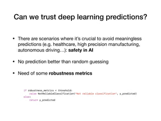
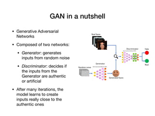
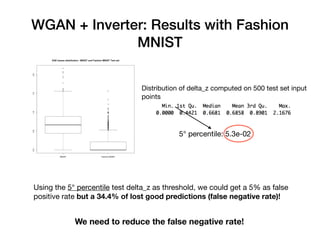
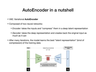
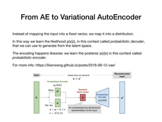
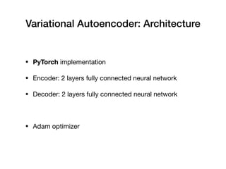
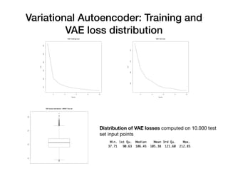
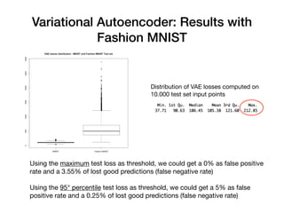
Davide Posillipo's presentation at the Milan AI meetup focused on robustness metrics for deep learning models, highlighting the need for reliable predictions in critical applications. He discussed two approaches for assessing model robustness: a GAN-based method that evaluates prediction stability and a variational autoencoder (VAE) that measures encoding-decoding loss to determine if new input data comes from the same distribution as the training set. The presentation emphasized that implementing effective robustness metrics will be essential for compliance with upcoming AI regulations in the EU.

1. Robustness Metrics for ML
Models based on Deep
Learning Methods
Davide Posillipo
Alkemy - Data Science Milan Meetup - AI Guild
21/07/2022, Milan

2. Who am I?
Hi! My name is Davide Posillipo.
I studied Statistics.
For 8+ years I’ve been working on
projects that require using data to
answer questions.
Freelancer Data Scientist and Teacher.
Currently building the Alkemy’s Deep
Learning & Big Data Department.
Happy to connect and work together on
new ideas and projects. Get in touch!

3. This event,
tonight

4. Let’s get started

5. MNIST: a simple case
• MNIST: solved problem
• LeNet: Deep Convolutional Neural Network, 99% accuracy
Predicted
digit

6. What happens if
we pass a
chicken to
LeNet?
The chicken comes from a
di
ff
erent distribution.
What should the model do?

7. What happens if we pass a chicken to LeNet?
We expect this output:
?

8. What happens if we pass a chicken to LeNet?
… but we obtain this result:
6, with probability 0.9

9. A less obvious example: Fashion MNIST
63.4% of examples are classi
fi
ed with a probability
greater than 0.99
74.3% of examples are classi
fi
ed with a probability
greater than 0.95
88.9% of examples are classi
fi
ed with a probability
greater than 0.75
LeNet (trained for MNIST) produces “con
fi
dent” predictions for the Fashion MNIST

10. Can we trust deep learning predictions?
• There are scenarios where it’s crucial to avoid meaningless
predictions (e.g. healthcare, high precision manufacturing,
autonomous driving…): safety in AI
• No prediction better than random guessing
• Need of some robustness metrics

11. Robustness metrics: how should it be?
A robustness metrics should tell us if the prediction is reliable or if it
is some sort of random guessing. It should provide some measure of
con
fi
dence in our prediction.
• Computable without labels
• Computable in “real-time”
• Easy to plug-in into a working ML pipeline
• Low false positive rate, but also low false negative rate
• High e
ff
ectiveness in detecting the anomaly points (low false negative
rate)
• Low rate of discarded “good predictions” (low false positive rate)

12. A few words about Robustness
Robustness: the quality of an entity that doesn’t break too easily if
stressed in some way.
Canonical approaches in Statistics involve some modi
fi
cation of
the predictive model/estimator (“If you get into a stressful
situation, handle it better”), with often a loss of performance as
side e
ff
ect.
Tonight we focus on a di
ff
erent approach: we don’t modify our
models but we protect them from threats (“Don’t get into stressful
situations”). We look for the chickens and keep them away from
our model.
Fight-or-
fl
ight(-or-freeze) response: we choose to
fl
y!

13. Lack of robustness is a risk
There is an increasing attention in risks
associated with AI applications.
EU proposed an AI regulation that could
become applicable to industry players starting
from 2024 (https://digital-
strategy.ec.europa.eu/en/policies/regulatory-
framework-ai)
The Commission is proposing the
fi
rst-ever
legal framework on AI, which addresses the
risks of AI and positions Europe to play a
leading role globally.
At some point, robustness will be a mandatory
requirements of ML models in production, and
lack of it will be considered a risk.

14. Robustness metrics: two approaches
• GAN-based approach
• Decide if a prediction is worth the risk, checking the
“stability” of the classi
fi
er for the new input data
• VAE-based approach
• Decide if a prediction is worth the risk, checking the true
“origin” of the new input data

15. First approach:
WGAN + Inverter

16. GAN in a nutshell
• Generative Adversarial
Networks
• Composed of two networks:
• Generator: generates
inputs from random noise
• Discriminator: decides if
the inputs from the
Generator are authentic
or arti
fi
cial
• After many iterations, the
model learns to create
inputs really close to the
authentic ones

17. A fancier GAN: WGAN
• Wasserstein Generative Adversarial Networks
• It use Wasserstein distance as GAN loss function
• Wasserstein Distance is a measure of the distance between two
probability distributions
• Fore more info: https://lilianweng.github.io/posts/2017-08-20-
gan/

18. • Train a Generator (from random noise to the input space)
• Train a Discriminator (it tries to understand if a point is true or
generated by the Generator)
• The Generator learns how to fool the Discriminator
• Train an Inverter (from the input space to the latent
representation)
• The Inverter learns how the Generator maps from the
random noise to the input space
Adding the Inverter

19. Approach 1: overview
and loss functions
WGAN Loss Function
Inverter Loss Function

20. WGAN + Inverter: robustness metrics
• Given a new data point x,
fi
nd the closest point to x in the latent space
that is, once translated back to the original space, able to confound the
classi
fi
er f
• Robustness metrics: the distance ( delta_z = z* - I(x) ) between these two
points, in the latent representation
• If delta_z is “small”, the classi
fi
er is not con
fi
dent about its prediction
(the classi
fi
er “changes its mind” too easily)
• If delta_z is “big”, the classi
fi
er is con
fi
dent about the prediction (the
classi
fi
er “knows what it wants”)
Rule: if delta_z < threshold then do not predict

21. WGAN + Inverter: Architecture
• PyTorch implementation
• Generator: 1 Fully Connected + 4 Transposed Conv. Layers
(strides = 2), ReLu activation func.
• Discriminator (“Critic”): 4 Conv. Layers (strides = 2) + 1 Fully
Connected, ReLu activation func.
• Inverter: 4 Conv. Layers (strides = 2) + 2 Fully Connected, ReLu
activation func.
• Adam optimizers for the three nets

22. WGAN + Inverter: Training and
distribution of delta_z
Distribution of delta_z computed on 500 test set
input points

23. WGAN + Inverter: Results
Distribution of delta_z computed on 500 test set input
points
Delta_z for the chicken: 1.8e-06 (< 5.3e-02)
Using the 5° percentile test delta_z as threshold, we could get a 5% as false
positive rate and discard the meaningless predictions for the chicken picture.
5° percentile: 5.3e-02

24. WGAN + Inverter: Results with Fashion
MNIST
Using the 5° percentile test delta_z as threshold, we could get a 5% as false
positive rate but a 34.4% of lost good predictions (false negative rate)!
Distribution of delta_z computed on 500 test set input
points
5° percentile: 5.3e-02
We need to reduce the false negative rate!

25. Second approach:
Variational AutoEncoder

26. AutoEncoder in a nutshell
• VAE: Variational AutoEncoder
• Composed of two neural networks:
• Encoder: takes the inputs and “compress” them in a deep latent representation
• Decoder: takes the deep representation and creates back the original input as
much as it can
• After many iterations, the model learns the best “latent representation” (kind of
compression) of the training data

27. From AE to Variational AutoEncoder
Instead of mapping the input into a
fi
xed vector, we map it into a distribution.
In this way we learn the likelihood p(x|z), in this context called probabilistic decoder,
that we can use to generate from the latent space.
The encoding happens likewise: we learn the posterior p(z|x) in this context called
probabilistic encoder.
For more info: https://lilianweng.github.io/posts/2018-08-12-vae/

28. Variational Autoencoder: robustness
metrics
The loss function of a variational autoencoder is an indirect measure of the probability
that an observation comes from the same distribution that generated the training set.
An “unlikely” input will have troubles in the encoding-decoding process = high loss
value.
Robustness metrics: loss function
• “Big” loss -> Not robust prediction: the new input data doesn’t come from the
training set underlying distribution
• “Small” loss -> Robust prediction: the new input data comes from the training
set underlying distribution
Notice that with this approach we don’t need the classi
fi
er f for the robustness metrics
computation!
Rule: if VAE_loss > threshold then do not predict

29. Variational Autoencoder: Architecture
• PyTorch implementation
• Encoder: 2 layers fully connected neural network
• Decoder: 2 layers fully connected neural network
• Adam optimizer

30. Variational Autoencoder: Training and
VAE loss distribution
Distribution of VAE losses computed on 10.000 test
set input points

31. Variational Autoencoder: Results
Distribution of VAE losses computed on 10.000 test
set input points
Using the maximum test loss as threshold, we could get a 0% as false positive
rate and discard the meaningless predictions for the chicken picture.
VAE loss for the chicken: 309.4 (>212)

32. Variational Autoencoder: Results with
Fashion MNIST
Distribution of VAE losses computed on
10.000 test set input points
Using the maximum test loss as threshold, we could get a 0% as false positive
rate and a 3.55% of lost good predictions (false negative rate)
Using the 95° percentile test loss as threshold, we could get a 5% as false
positive rate and a 0.25% of lost good predictions (false negative rate)

33. Variational Autoencoder: robustness
metrics into production
• Train your classi
fi
er
• Train a VAE on your training set
• Get the distribution of the VAE losses on your test set
• De
fi
ne a threshold more or less “conservative”
• Implement a “conditional classi
fi
er”:

34. Conclusions

35. Wrapping up: pros and cons of this
approach
Pros
• No need to modify your predictive models
• The same “monitoring” system can be used for di
ff
erent ML
models (for a given dataset)
• Applicable to any kind of data (tabular, images, …)
• “Easy” to explain
• Easy to plug-in into existing pipelines
Cons
• Arbitrary thresholds must be set by the data scientist
• Introducing a further model that needs to be maintained

36. Thank you for your
attention!
https://www.linkedin.com/in/davide-posillipo/