Download as PDF, PPTX
![Hazard function
h(t) = 𝖯[T= t | T ≥ t]
Probability failure will happen at time t given that we know
it survived up to time t.
Can be interpreted as a measure of the hazard risk, aka.
the probability that failure would happen right now.](https://image.slidesharecdn.com/deeptime-to-failure-181123095551/75/Deep-time-to-failure-predicting-failures-churns-and-customer-lifetime-with-RNN-by-Gianmario-Spacagna-Chief-Scientist-at-Cubeyou-AI-15-2048.jpg)
![Cumulative Hazard function
Λ(t)=∫[0 to t] h(z) dz
Represents the integral of the hazard-rate.](https://image.slidesharecdn.com/deeptime-to-failure-181123095551/75/Deep-time-to-failure-predicting-failures-churns-and-customer-lifetime-with-RNN-by-Gianmario-Spacagna-Chief-Scientist-at-Cubeyou-AI-16-2048.jpg)

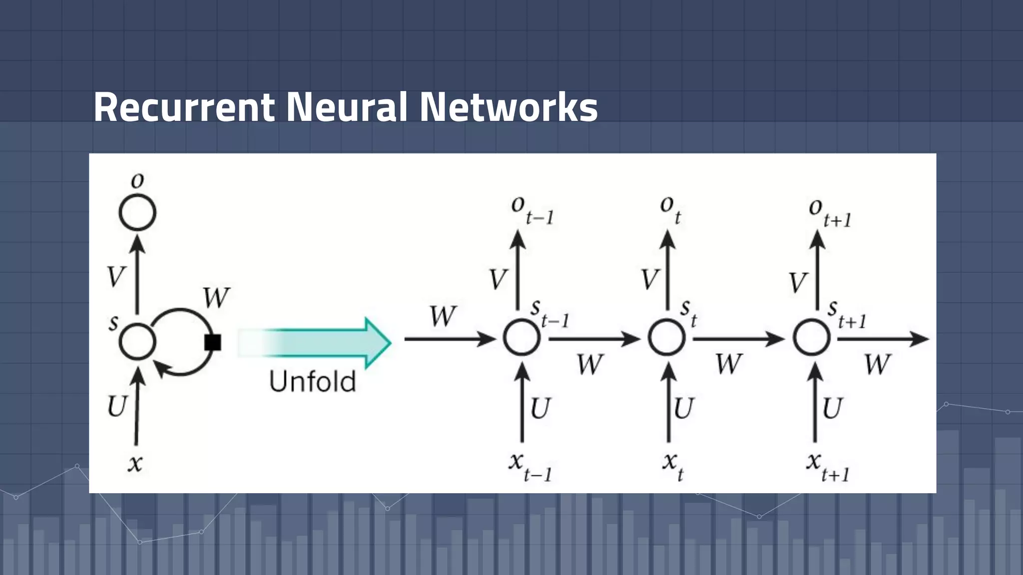
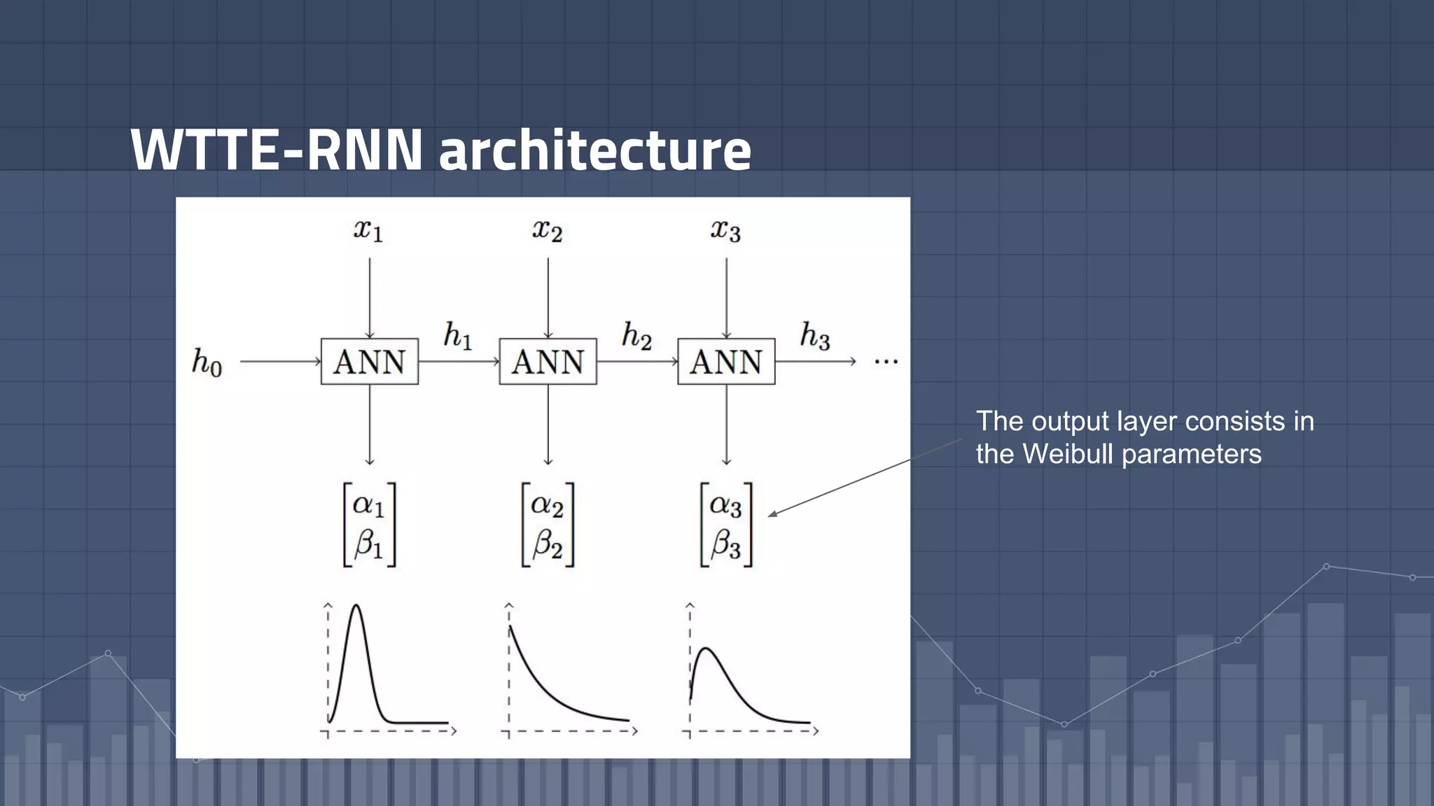
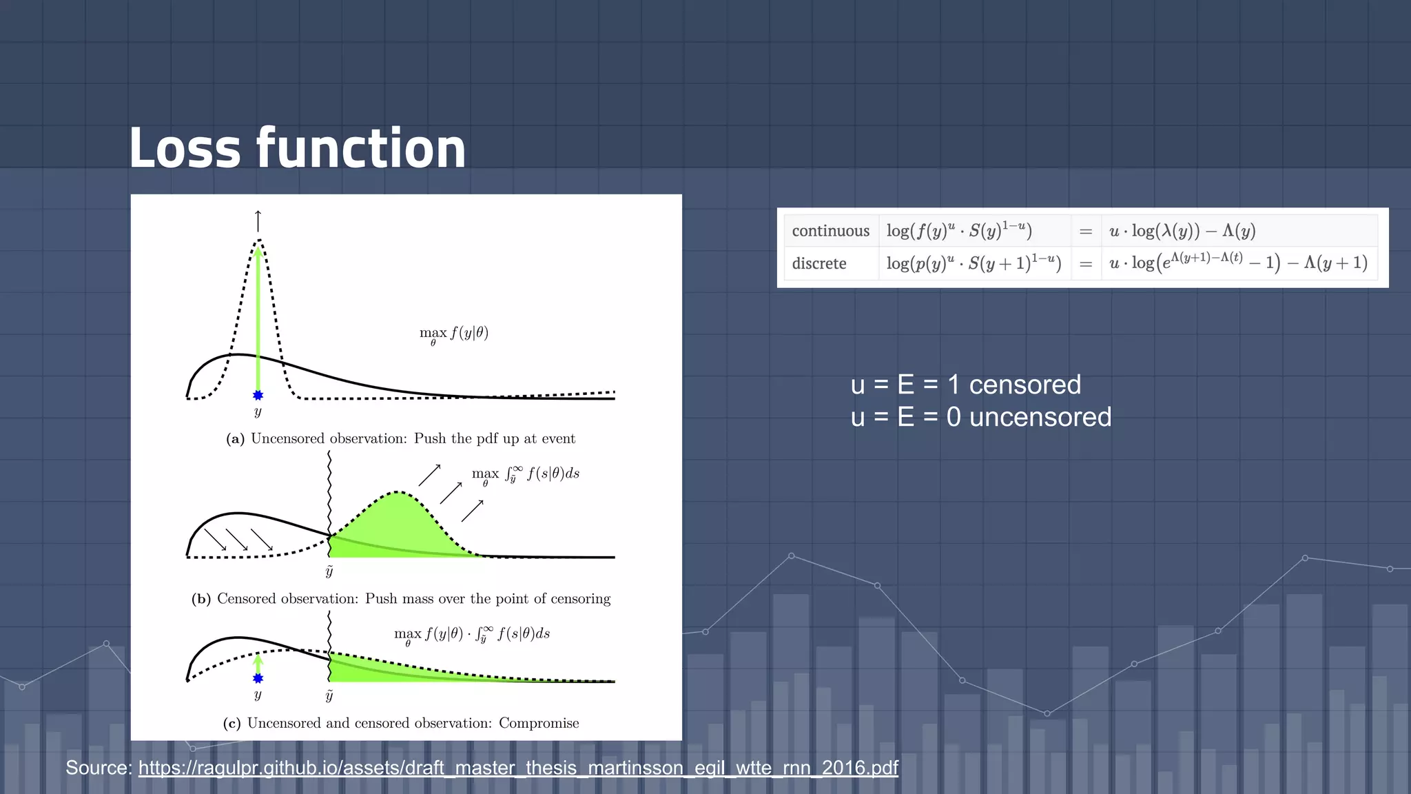
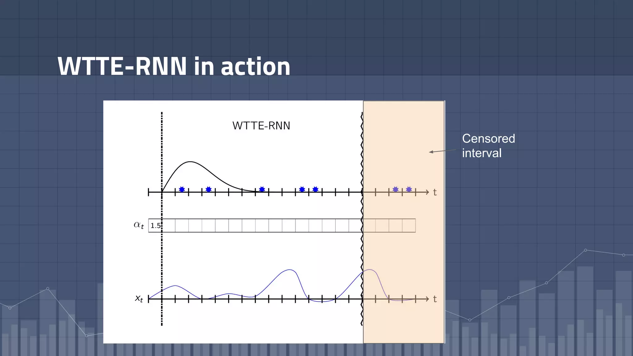
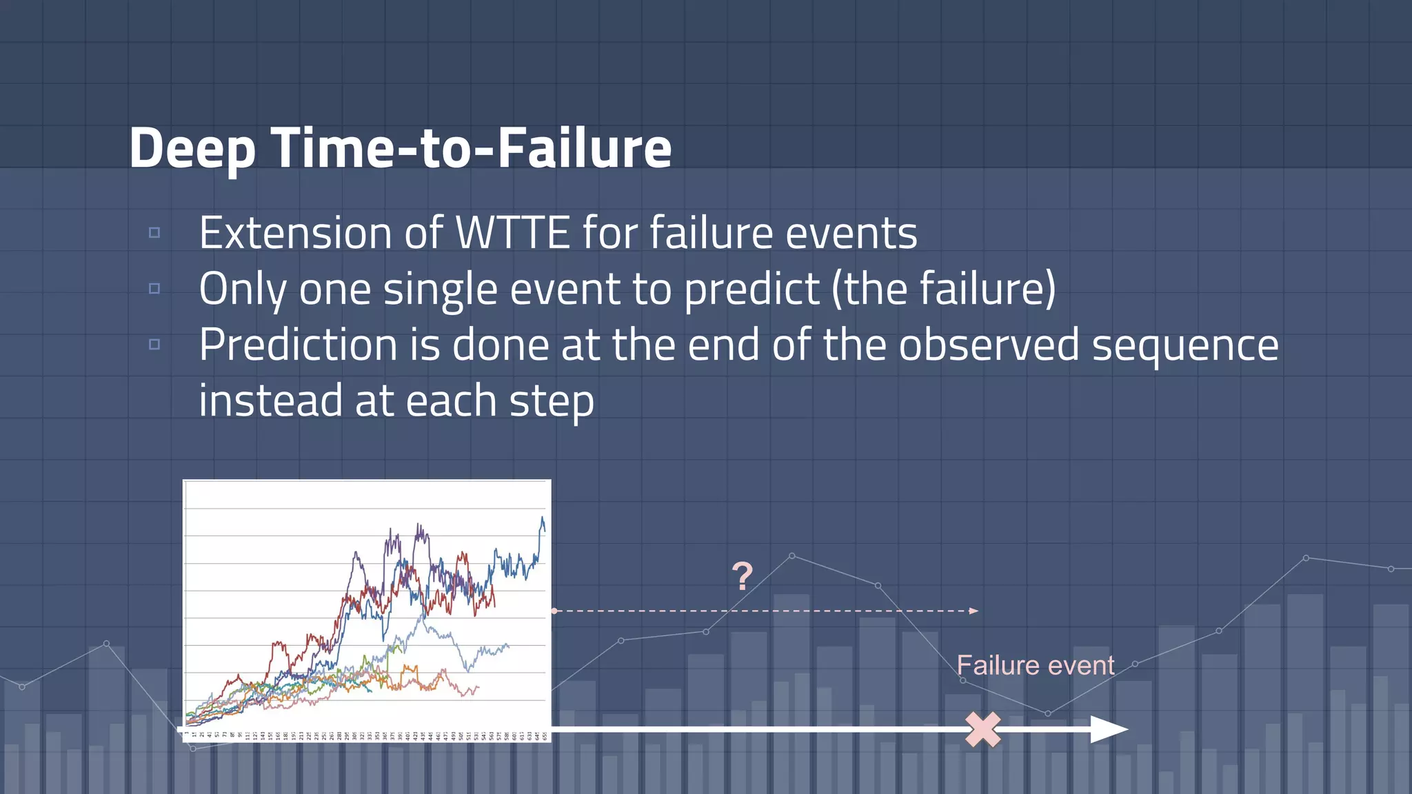
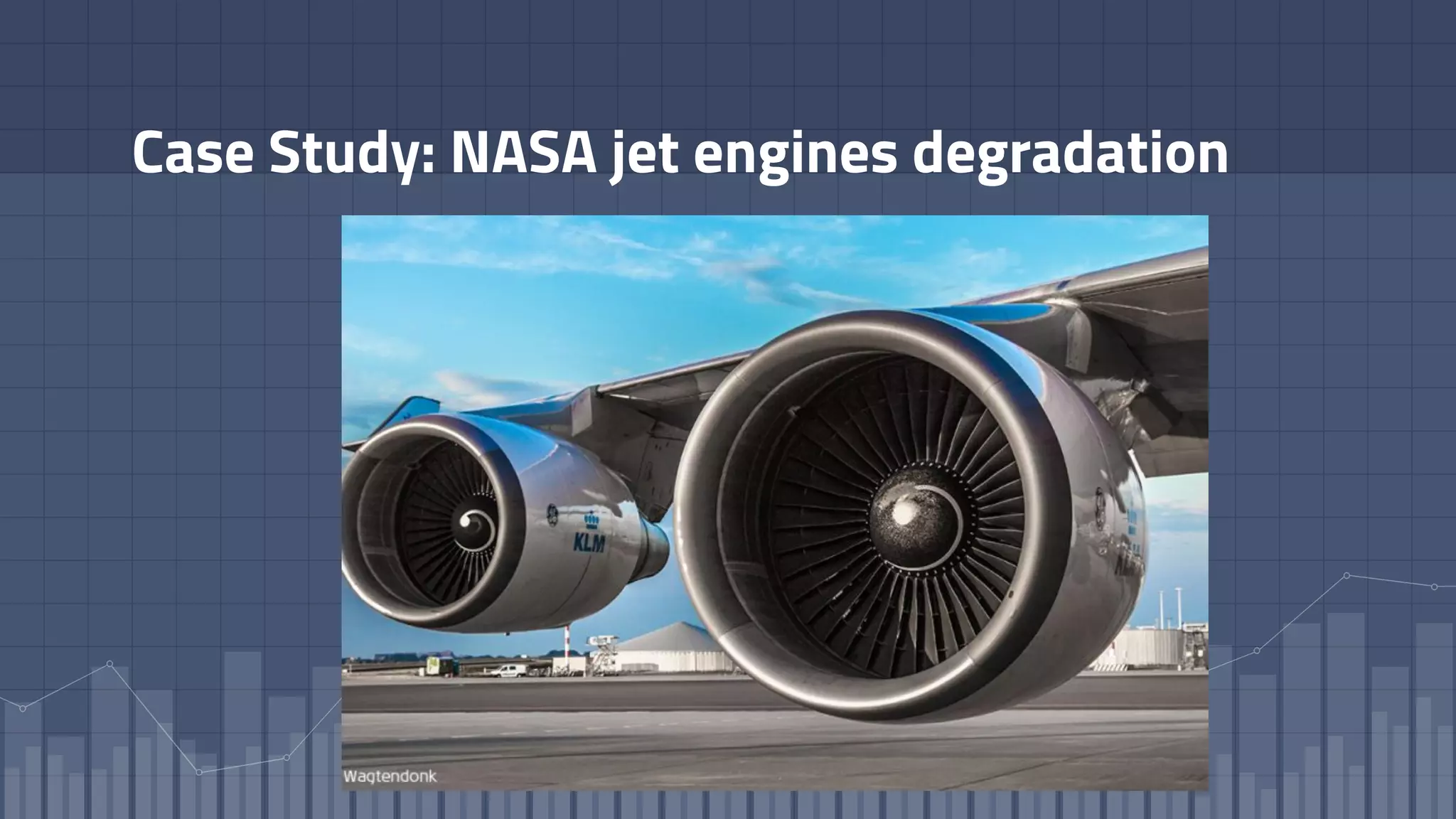

1. The document discusses using deep learning models like recurrent neural networks to predict time-to-failure events from time series data. It specifically focuses on a technique called Deep Time-to-Failure which extends a Weibull Time-to-Event Recurrent Neural Network to predict a single failure event. 2. As a case study, the technique is applied to predict failure times of NASA jet engines using sensor data as inputs. The model is trained on historical sequences of data to learn the distribution of time-to-failure and can provide probabilistic predictions and confidence intervals. 3. Key aspects of the Deep Time-to-Failure approach include using censored and uncensored training data, consuming raw time series as input
![ARIMA Models - [Lab 3]](https://cdn.slidesharecdn.com/ss_thumbnails/ydqcxn5vtqizjoun2as1-signature-e1de5ad681d661531c2467ca0d3e475440809ccfdbcb78c5369a1bb749945888-poli-141230090527-conversion-gate01-thumbnail.jpg?width=640&height=640&fit=bounds)


![Sensor Fusion Study - Ch8. The Continuous-Time Kalman Filter [이해구]](https://cdn.slidesharecdn.com/ss_thumbnails/chapter8-thecontinuoustimekalmanfilter-200715035017-thumbnail.jpg?width=640&height=640&fit=bounds)