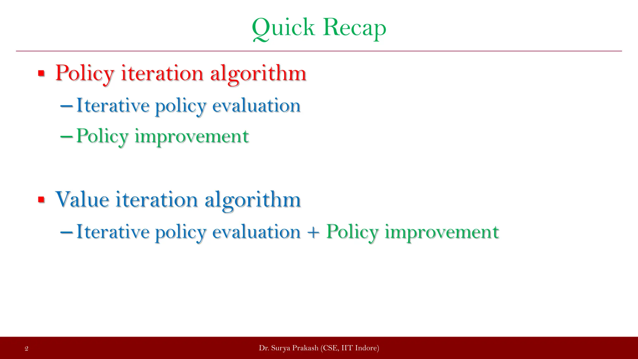
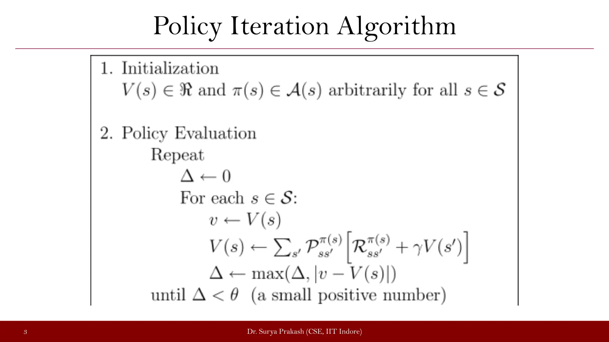
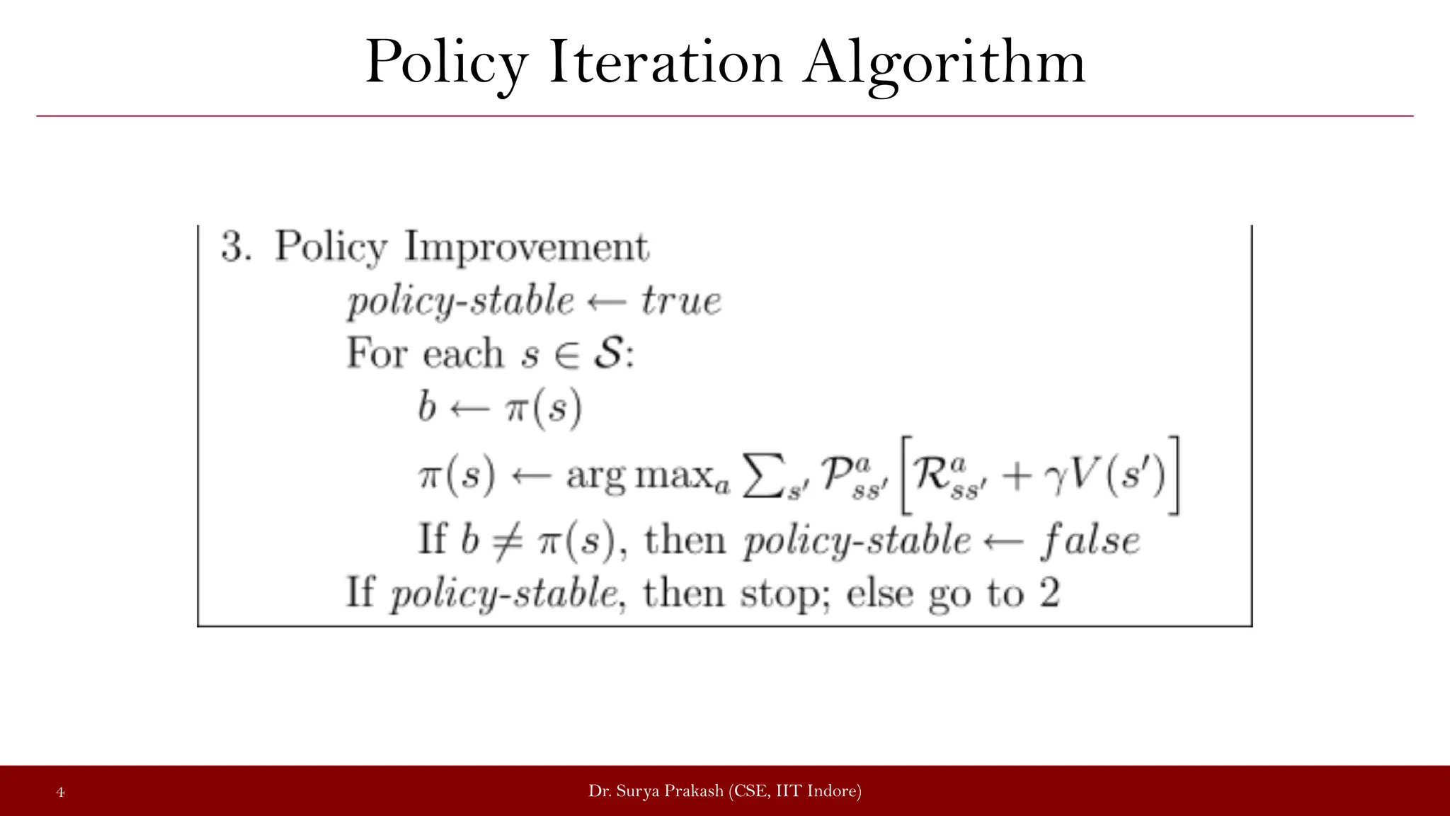
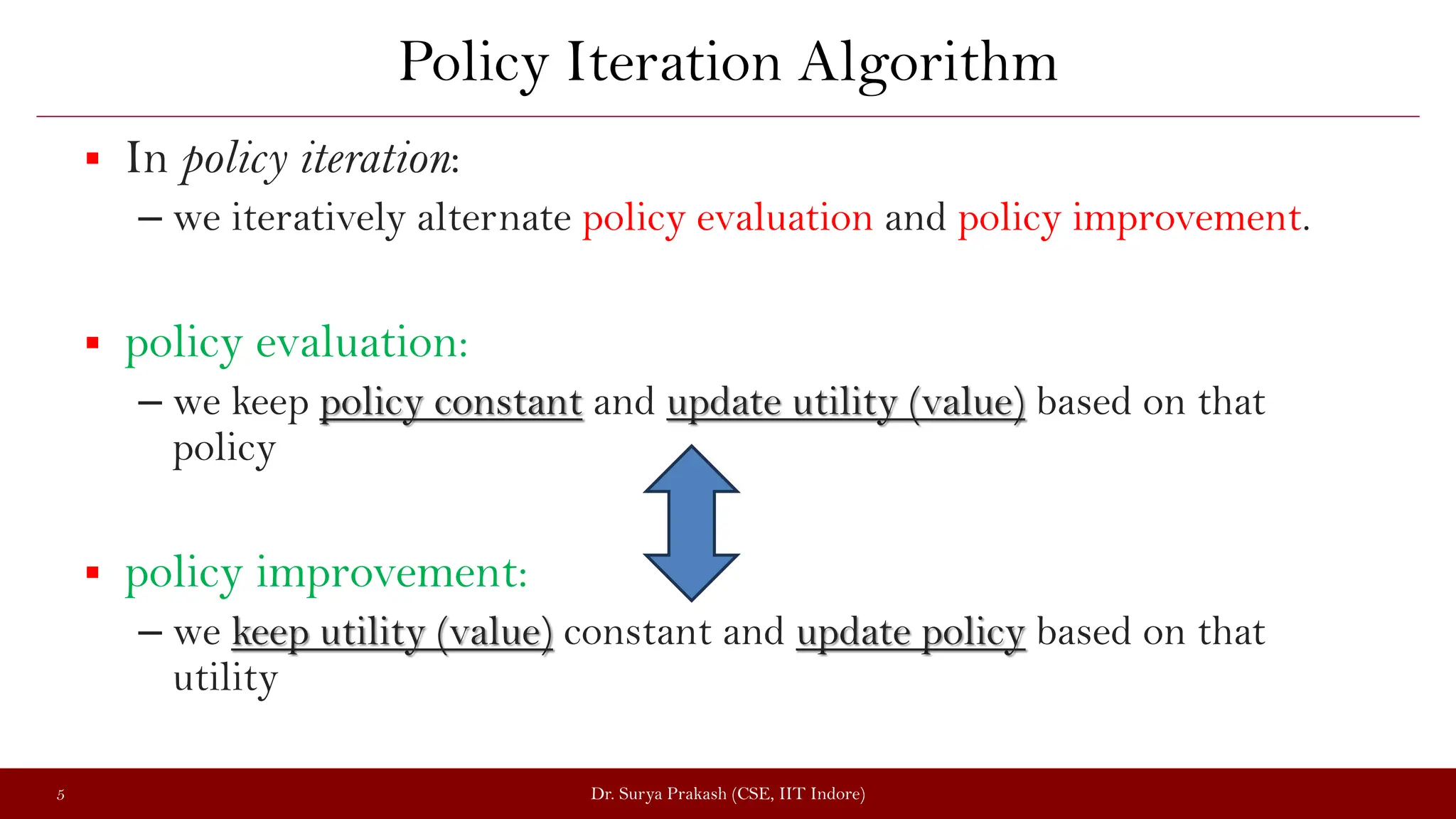
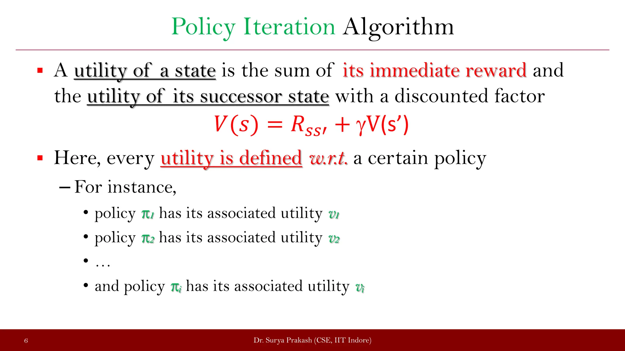
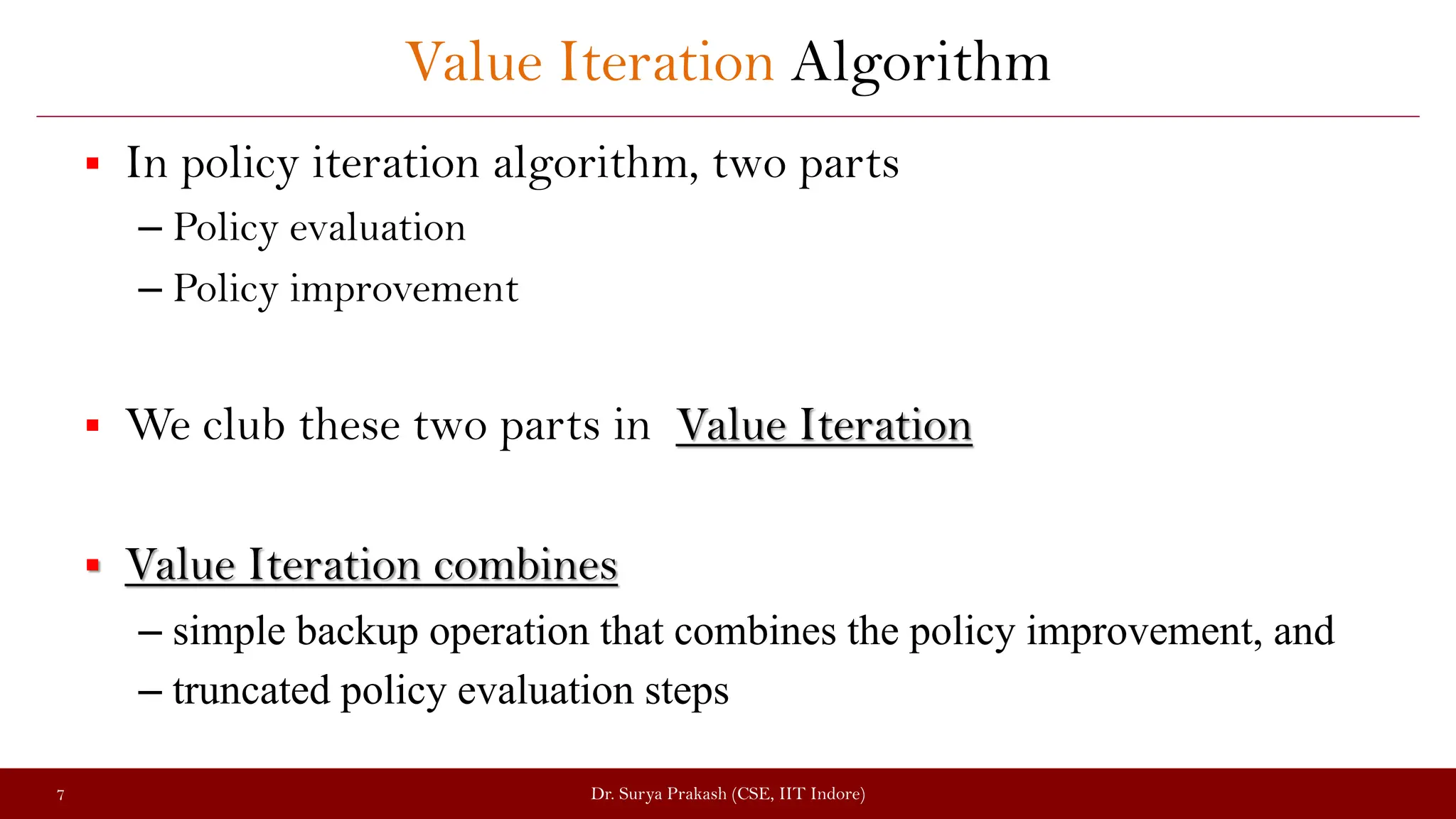
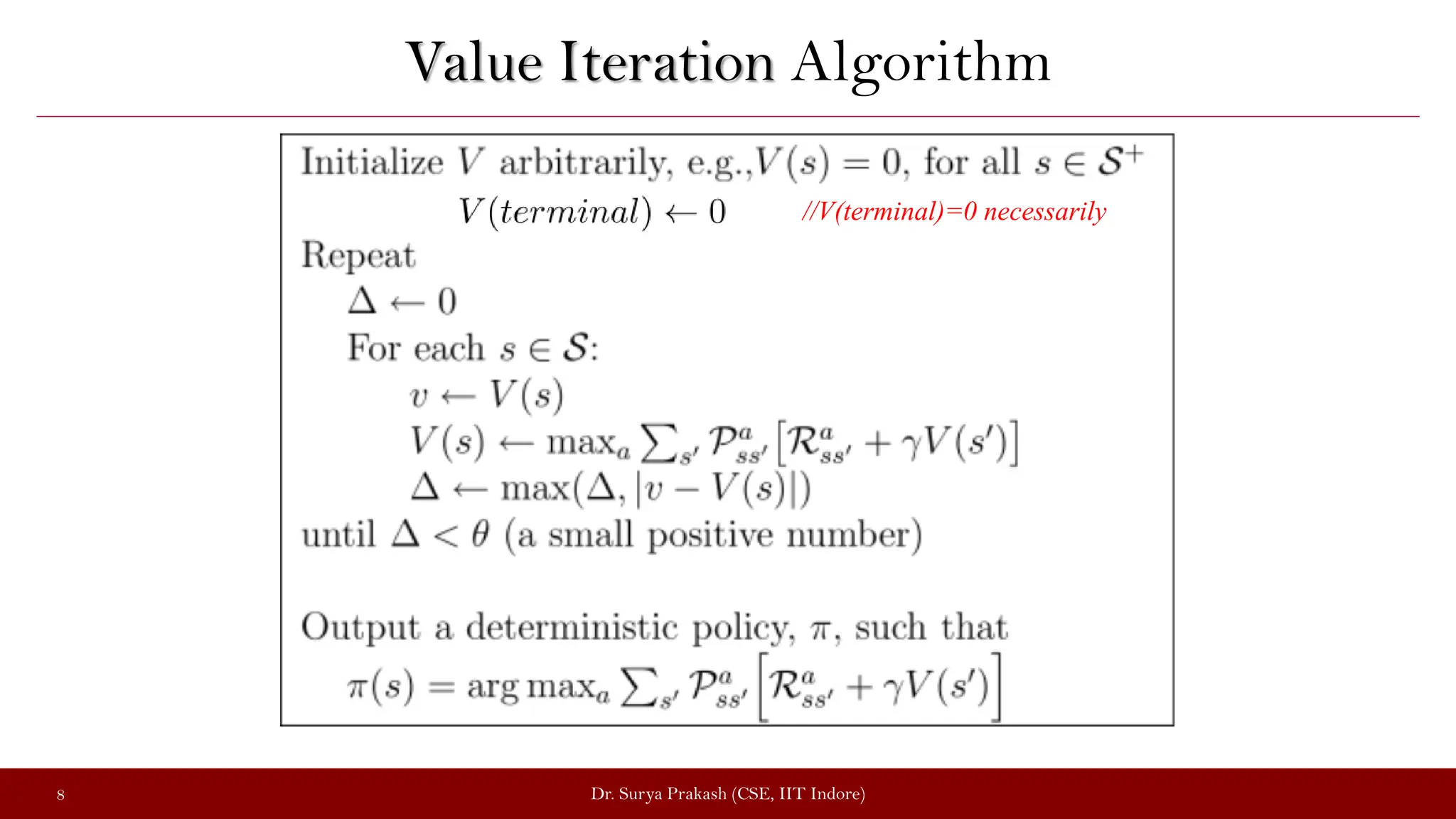
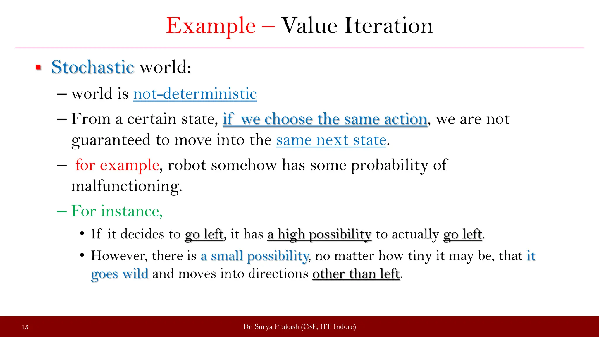
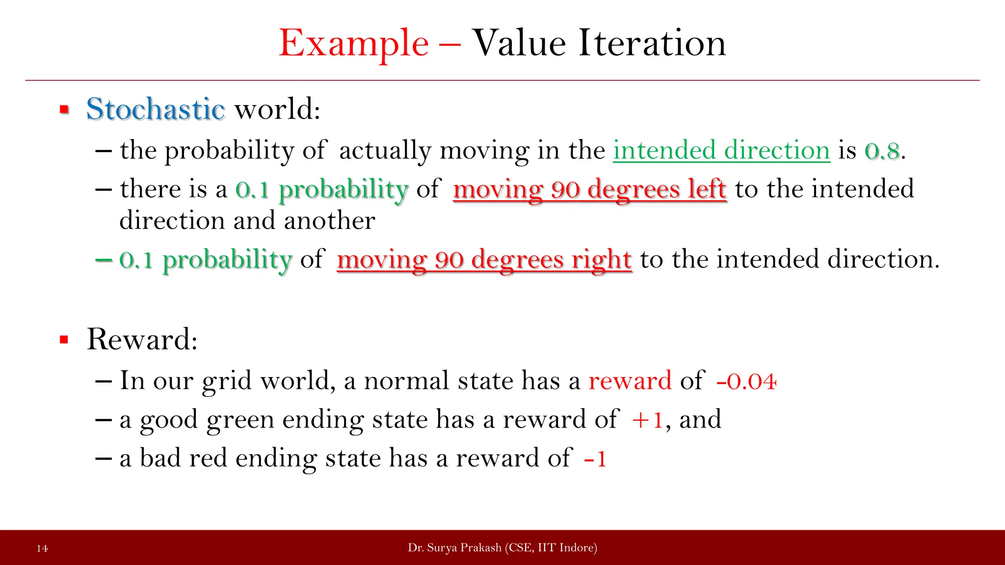
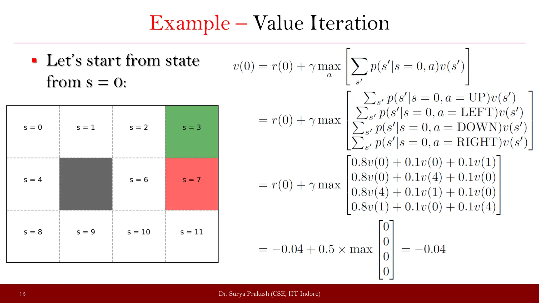
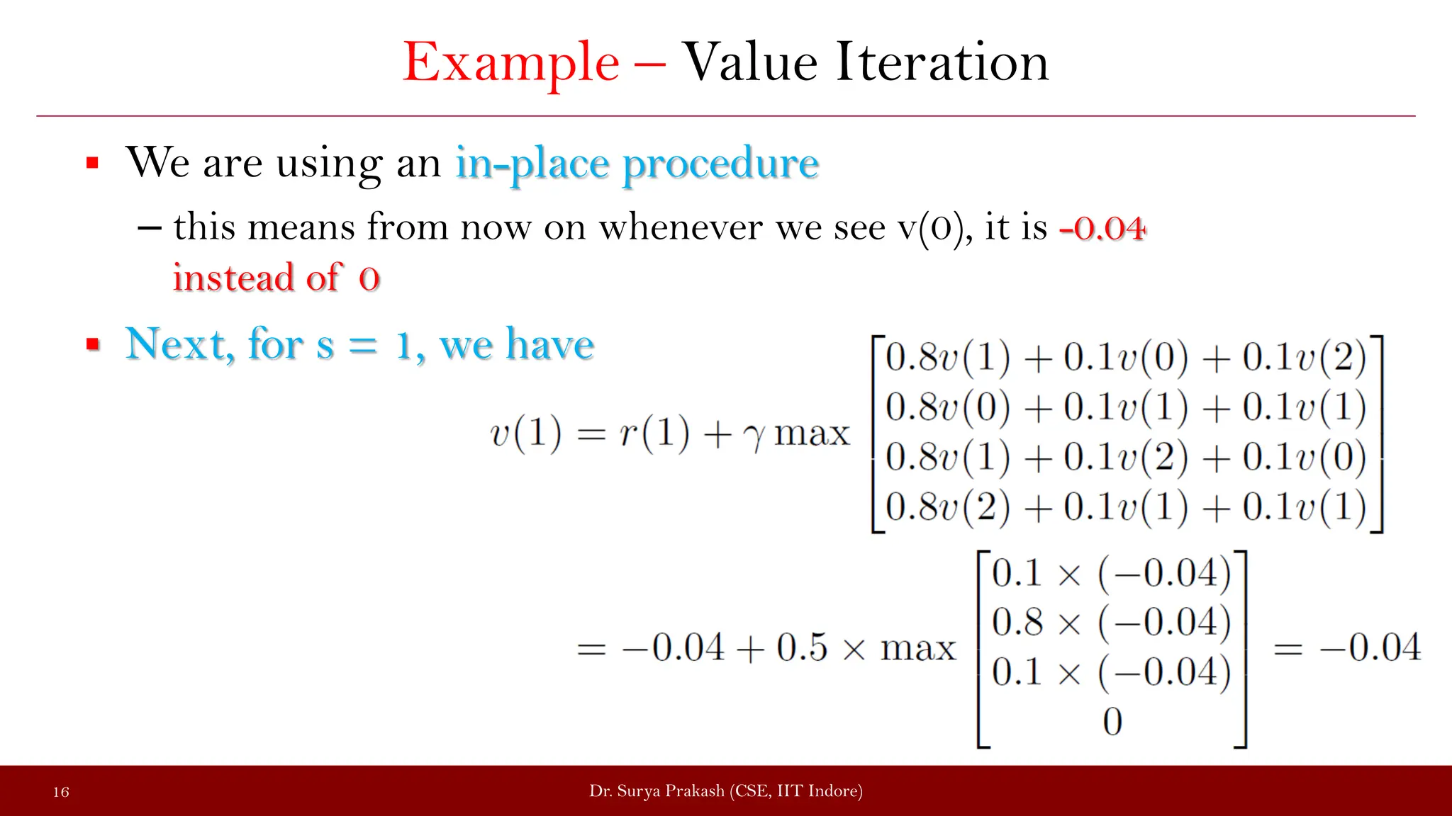
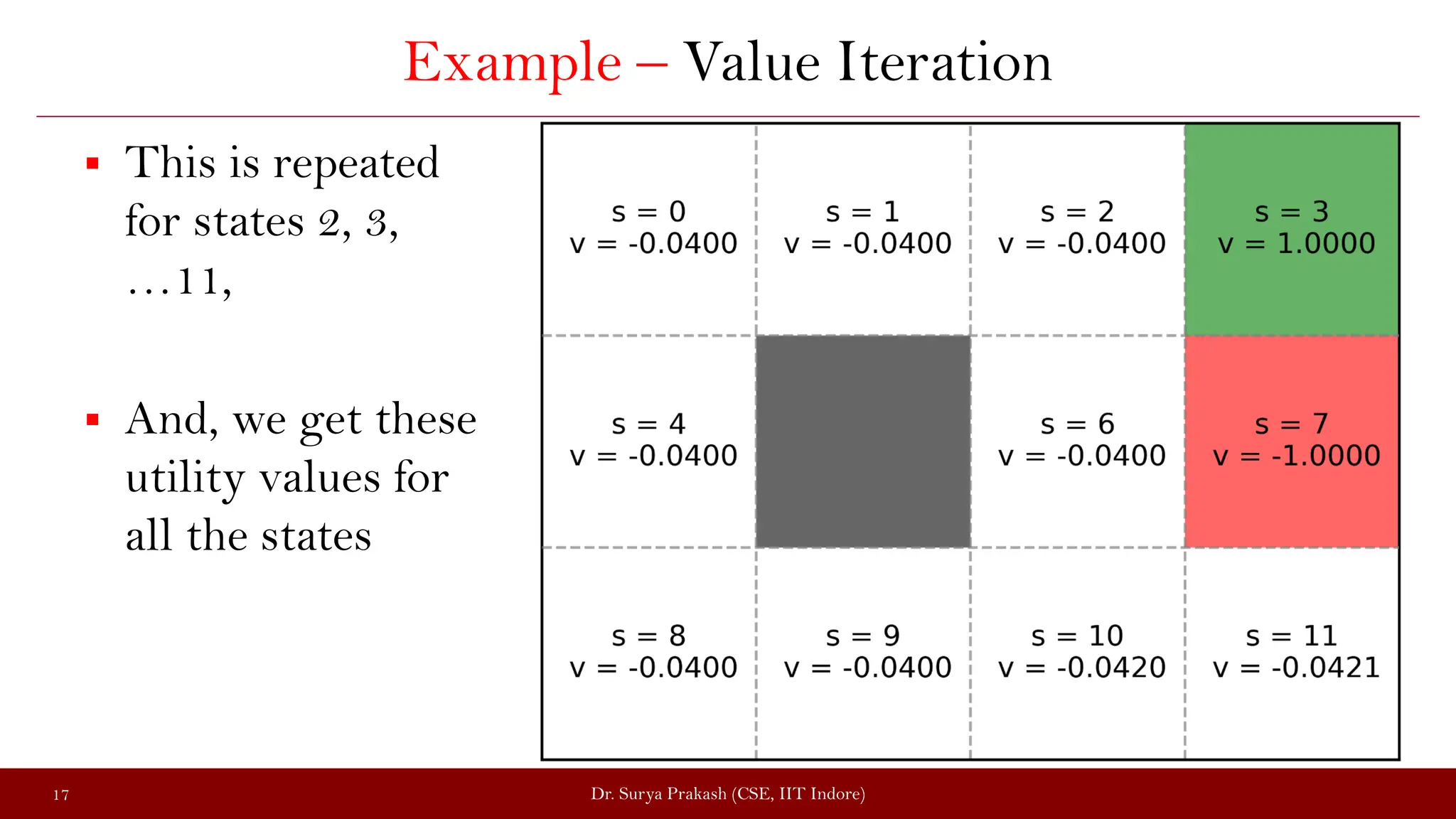
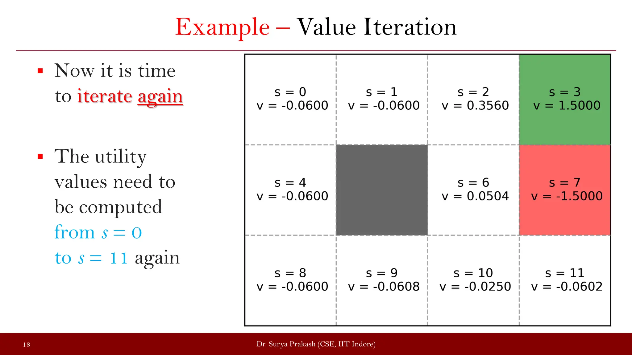
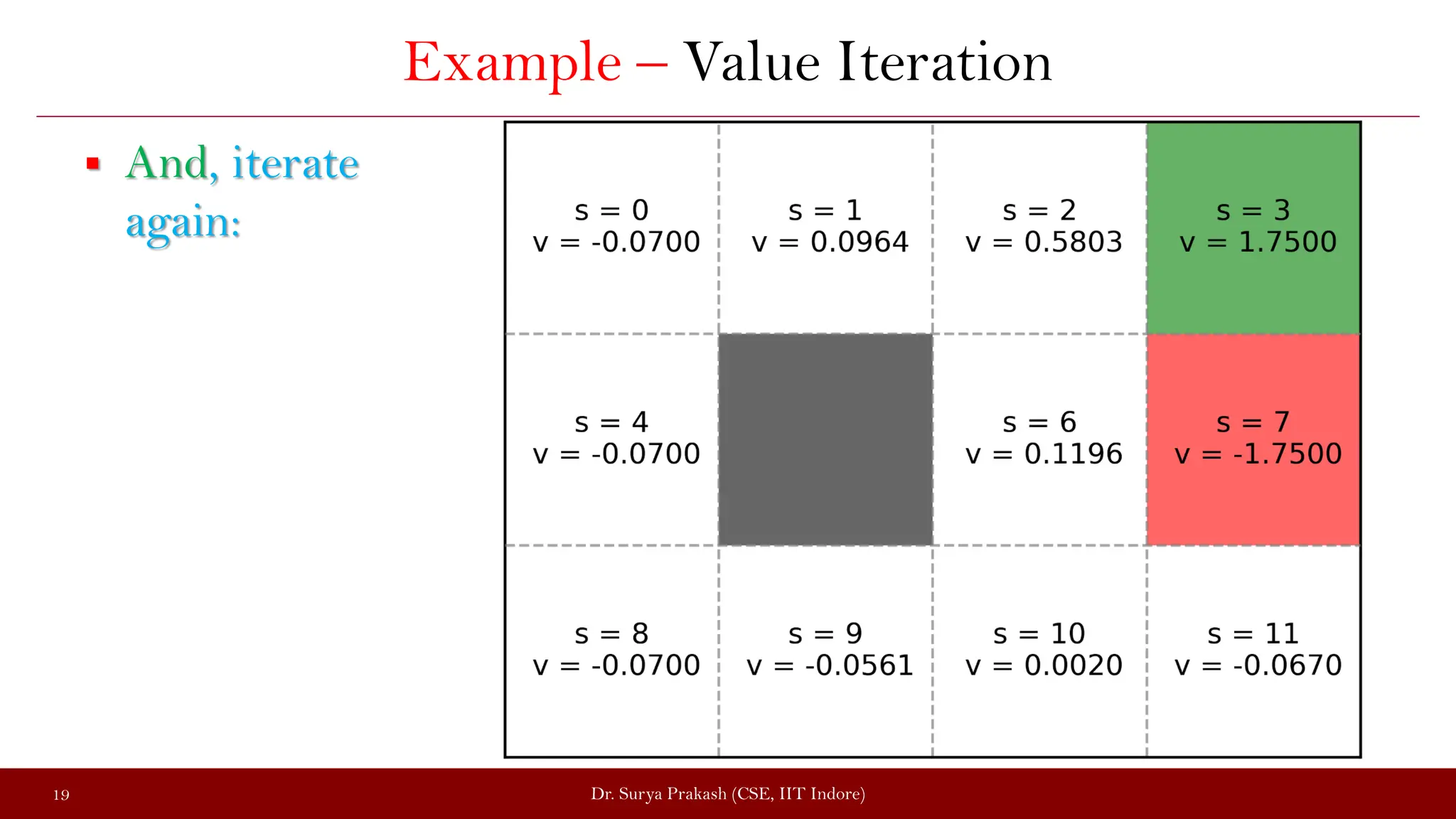
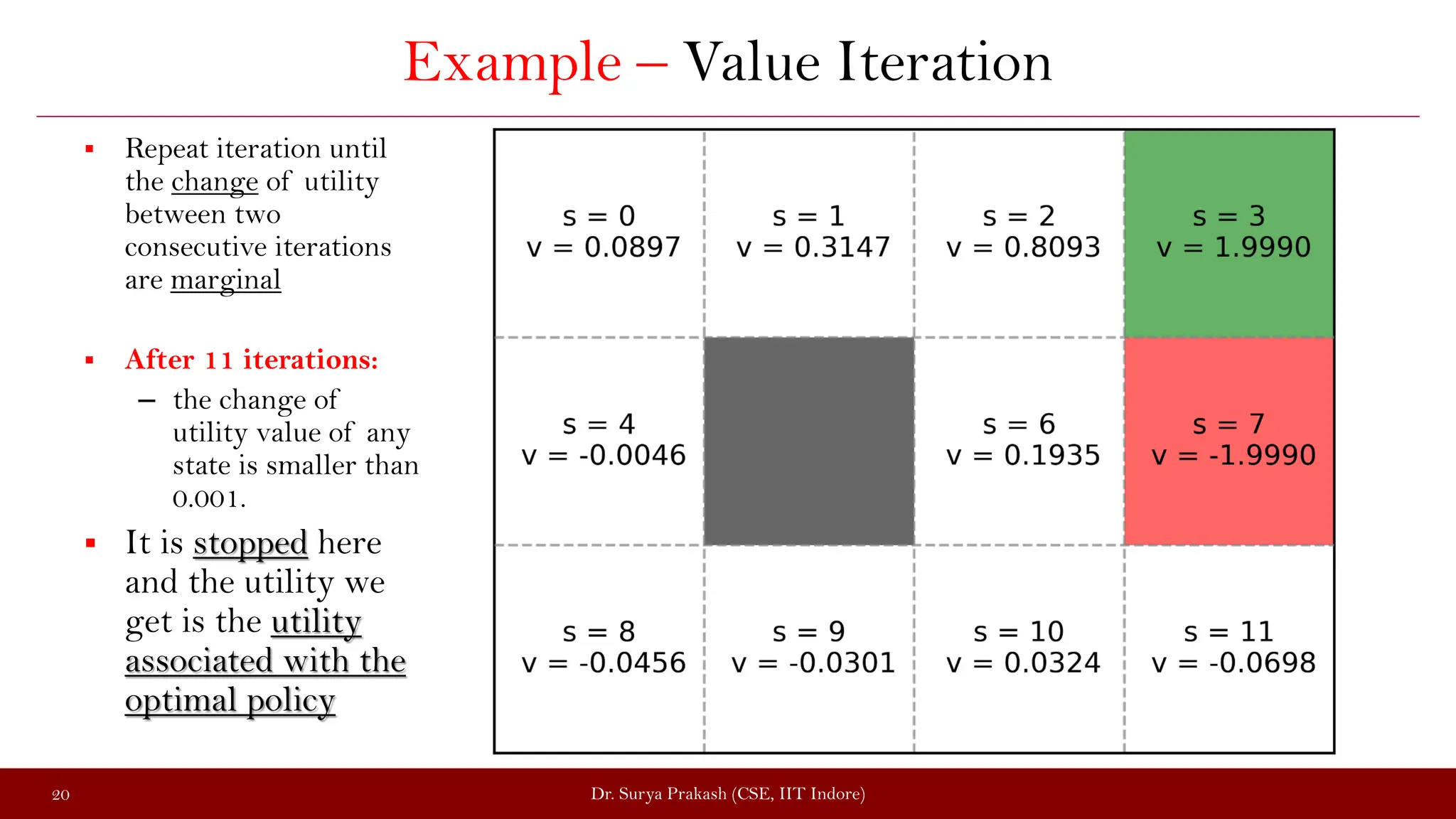
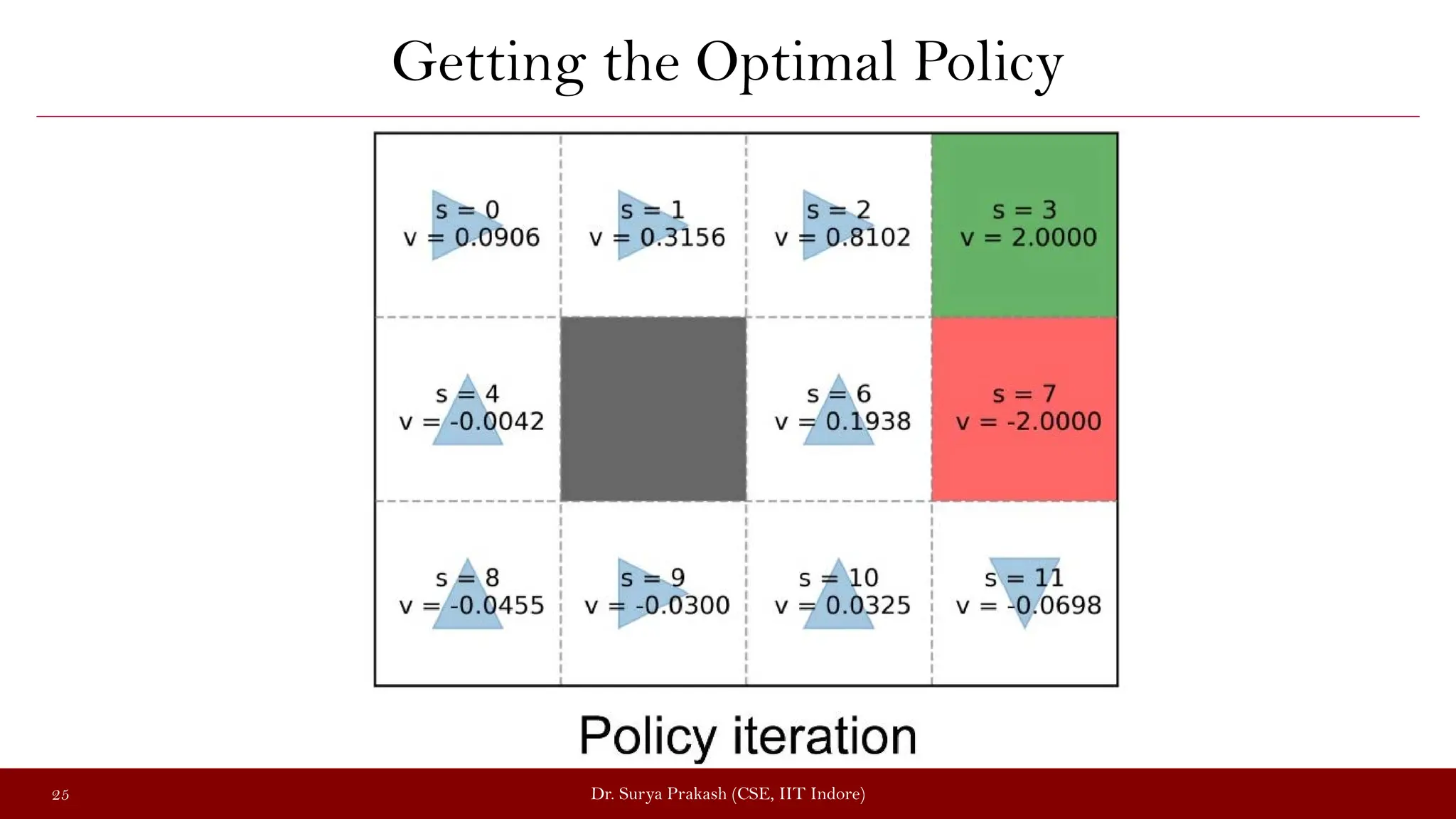
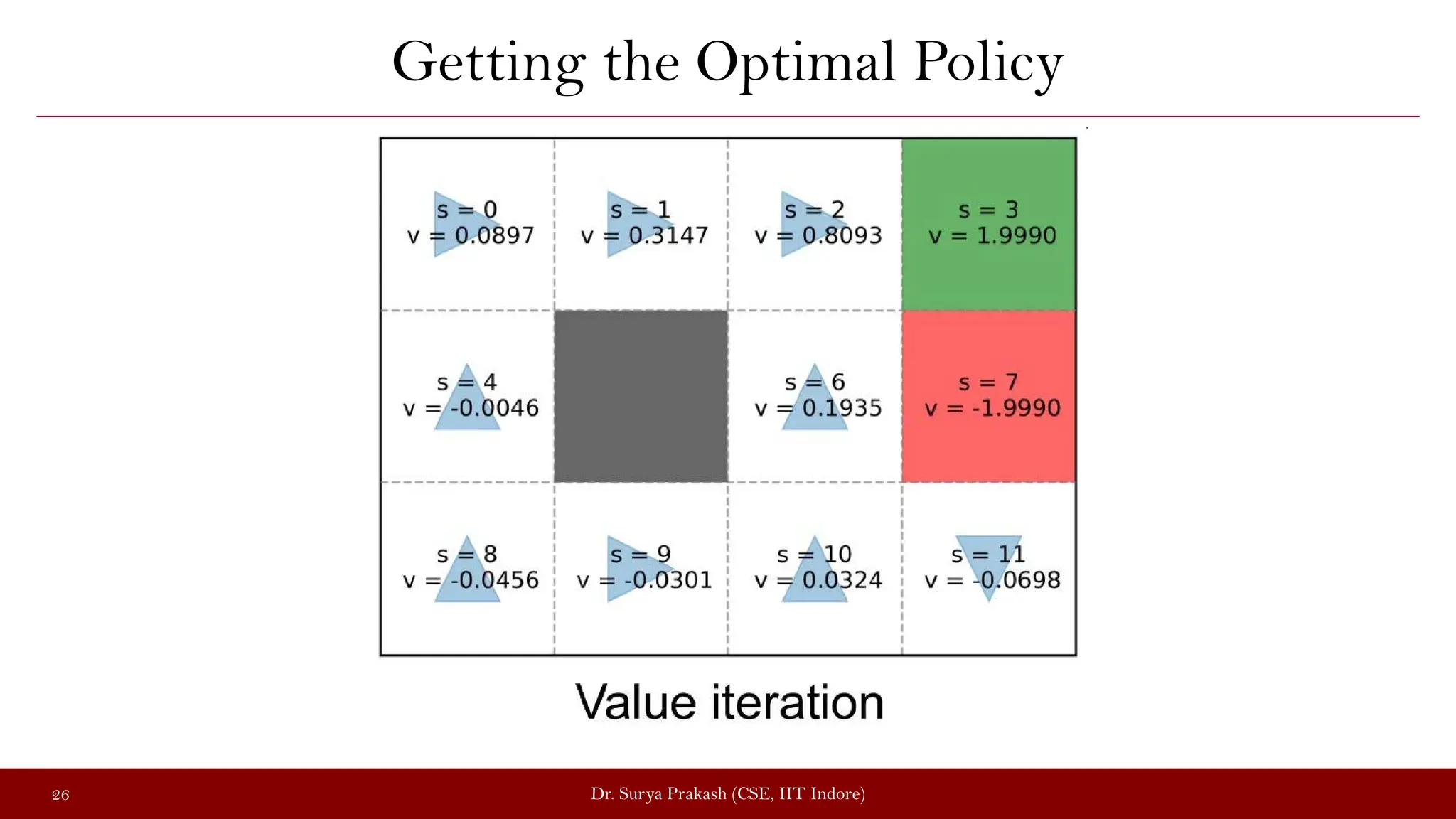
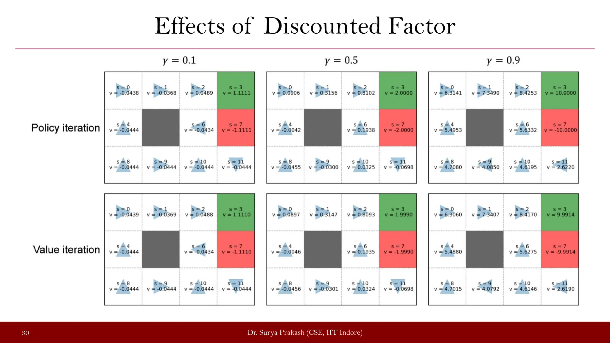
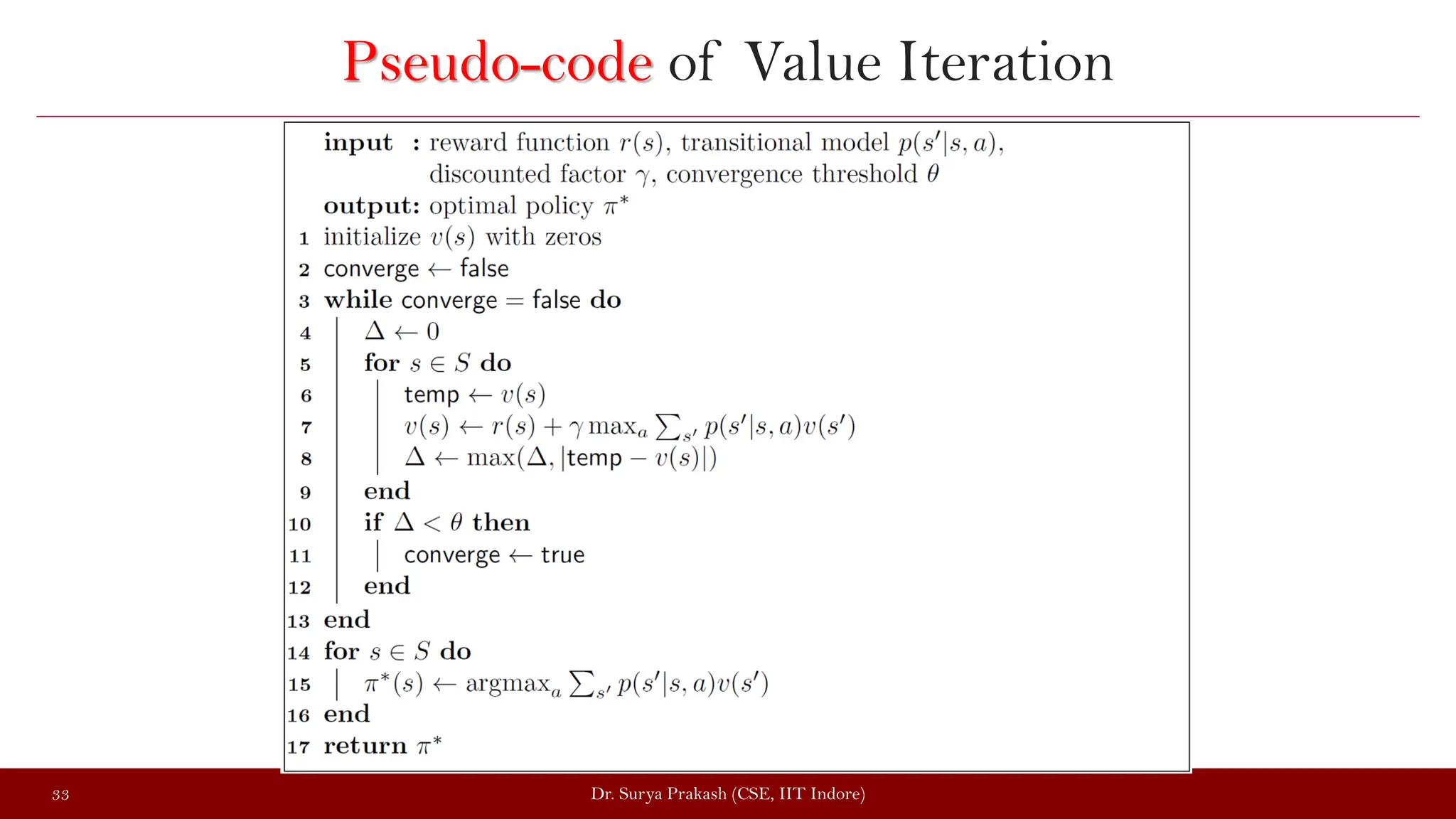
mathematics, a Markov decision process (MDP) is a discrete-time stochastic control process. It provides a mathematical framework for modeling decision making in situations where outcomes are partly random and partly under the control of a decision maker. MDPs are useful for studying optimization problems solved via dynamic programming. MDPs were known at least as early as the 1950s;[1] a core body of research on Markov decision processes resulted from Ronald Howard's 1960 book, Dynamic Programming and Markov Processes.[2] They are used in many disciplines, including robotics, automatic control, economics and manufacturing. The name of MDPs comes from the Russian mathematician Andrey Markov as they are an extension of Markov chains.
At each time step, the process is in some state
�
{\displaystyle s}, and the decision maker may choose any action
�
{\displaystyle a} that is available in state
�
{\displaystyle s}. The process responds at the next time step by randomly moving into a new state
�
′
{\displaystyle s'}, and giving the decision maker a corresponding reward
�
�
(
�
,
�
′
)
{\displaystyle R_{a}(s,s')}.
The probability that the process moves into its new state
�
′
{\displaystyle s'} is influenced by the chosen action. Specifically, it is given by the state transition function
�
�
(
�
,
�
′
)
{\displaystyle P_{a}(s,s')}. Thus, the next state
�
′
{\displaystyle s'} depends on the current state
�
{\displaystyle s} and the decision maker's action
�
{\displaystyle a}. But given
�
{\displaystyle s} and
�
{\displaystyle a}, it is conditionally independent of all previous states and actions; in other words, the state transitions of an MDP satisfy the Markov property.
Markov decision processes are an extension of Markov chains; the difference is the addition of actions (allowing choice) and rewards (giving motivation). Conversely, if only one action exists for each state (e.g. "wait") and all rewards are the same (e.g. "zero"), a Markov decision process reduces to a Markov chain.equations. These equations are merely obtained by making
�
=
�
′
{\displaystyle s=s'} in the step two equation.[clarification needed] Thus, repeating step two to convergence can be interpreted as solving the linear equations by relaxation.
This variant has the advantage that there is a definite stopping condition: when the array
�
{\displaystyle \pi } does not change in the course of applying step 1 to all states, the algorithm is completed.
Policy iteration is usually slower than value iteration for a large number of possible states.
Modified policy iteration
edit
In modified policy iteration (van Nunen 1976; Puterman & Shin 1978), step one is performed once, and then step two is repeated several times.[9][10] Then step one is again performed once and so on.
Prioritized sweeping
edit
In this variant, the steps are preferentially applied to states which are in some way important – whether based on the algorithm (there were large changes in In this variant,
Policy iteration
Overview
Policy evaluation
Policy improvement
Policy iteration
Implementation
Takeaways
Video byte: Introduction to policy-based approaches and policy iteration
Learning outcomes
The learning outcomes of this chapter are:
Apply policy iteration to solve small-scale MDP problems manually and program policy iteration algorithms to solve medium-scale MDP problems automatically.
Discuss the strengths and weaknesses of policy iteration.
Compare and contrast policy iteration to value iteration.
Overview
Video byte: Intuition of policy-based approaches
The other common way that MDPs are solved is using policy iteration – an approach that is similar to value iteration. While value iteration iterates over value functions, policy iteration iterates over policies themselves, creating a strictly improved policy in each iteration (except if the iterated policy is already optimal).
Policy iteration first starts with some (non-optimal) policy, such as a random policy, and then calculates the value of each state of the MDP given that policy — this step is called policy evaluation. It then updates the policy itself for every state by calculating the expected reward of each action applicable from that state.
The basic idea here is that policy evaluation is easier to computer than value iteration because the set of actions to consider is fixed by the policy that we have so far.
Policy evaluation
Video byte: Model-based policy evaluation
An important concept in policy iteration is policy evaluation, which is an evaluation of the expected reward of a policy.
The expected reward of policy
from
,
, is the weighted average of reward of the possible state sequences defined by that policy times their probability given
.
Definition – Policy evaluation
Policy evaluation can be characterised as
as defined by the following equation:
where
for terminal states.
Note that this is very similar to the Bellman equation, except
is not the value of the best action, but instead just as the value for
, the action that would be chosen in
by the policy
. Note the expression
instead of
, which means we only evaluate the action that the policy defines.
Once we understand the definition of policy evaluation, the implementation is straightforward. It is the same as value iteration except that we use the policy evaluation equation instead of the Bellman equation.
Algorithm 11 (Policy evaluation)
Reinforcement learning
Reinforcement learning is an area of Machine Learning. It is about taking suitable action to maximize reward in a particular situation. It is employed by various software and machines to find the best possible behavior or path it should take in a specific situation. Reinforcement learning differs from supervised learning in a way that in supervised learning the training data has the answer key with it so the model is trained with the correct answer itself whereas in reinforcement learning, there is no answer but the
active. The environment may refer to an actual physical system or a simulated environment. Once the environment is determined, experimentation can begin for the RL process.
Step II: Specify the reward
In the next step, you need to define the reward for the agent. It acts as a performance metric for the agent and allows the agent to evaluate the task quality against its goals. Moreover, offering appropriate rewards to the agent may require a few iterations to finalize the right one for a specific action.
Step III: Define the agent
Once the environment and rewards are finalized, you can create the agent that specifies the policies involved, including the RL training algorithm. The process can include the following steps:
Use appropriate neural networks or lookup tables to represent the policy
Choose the suitable RL training algorithm
Step IV: Train/Validate the agent
Train and validate the agent to fine-tune the training policy. Also, focus on the reward structure RL design policy architecture and continue the training process. RL training is time-intensive and takes minutes to days based on the end application. Thus, for a complex set of applications, faster training is achieved by using a system architecture where several CPUs, GPUs, and computing systems run in parallel.
Step V: Implement the policy
Policy in the RL-enabled system serves as the decision-making component deployed using C, C++, or CUDA development code.
While implementing these policies, revisiting the initial stages of the RL workflow is sometimes essential in situations when optimal decisions or results are not achieved.
The factors mentioned below may need fine-tuning, followed by retraining of the agent:
RL algorithm configuration
Reward definition
Action / state signal detection
Environmental variables
Training structure
Policy framework.
Machine Learning Tutorial
Data Analysis Tutorial
Python - Data visualization tutorial
NumPy
Pandas
OpenCV
R
Machine Learning Projects
Machine Learning Interview Questions
Machine Learning Mathematics
Deep Learning Tutorial
Deep Learning Project
Deep Learning Interview Questions
Computer Vision Tutorial
Computer Vision Projects
NLP
NLP Project
NLP Interview Questions
Statistics with Python
100 Days of Machine Learning
▲
Open In App
Job Fair 2024
Share Your Experience
Machine Learning Tutorial
Getting Started with Machine Learning
Machine Learning Mathematics
Data Preprocessing
Classification & Regression
K-Nearest Neighbors (KNN)
Support Vector Machines
Decision Tree
Ensemble Learning
Generative Model
Time Series Forecasting
Clustering Algorithm
Convolutional Neural Networks
Recurrent Neural Networks
Reinforcement Learning
Reinforcement learning
Markov Decision Process
Q-Learning in Python
Deep Q-Learning
Deep Learning Tutorial
Computer Vision Tutorial
Natural Language Processing (NLP) Tutorial
Model Deployment and Productionization
Advanced Topics
100 Days of Machine Learning - A Complete Guide For Beginners
100+ Machine Learning
Reinforcement learning involves an agent learning how to behave through trial-and-error interactions with an environment. The agent receives rewards or punishments without being told the correct actions. There are two main types of learning - supervised learning where examples are provided, and reinforcement learning where only evaluations are provided. Reinforcement learning can be modeled as a Markov decision process and approached through model-based methods which learn the environment model, or model-free methods like temporal difference learning which learn directly from experiences. Active learning requires an agent to consider the impact of actions on both immediate and long-term rewards. Exploration strategies balance exploiting current knowledge with exploring unknown areas. Generalization techniques like function approximation can help scale reinforcement learning to large problems.
This document provides an overview of reinforcement learning concepts. It introduces reinforcement learning as using rewards to learn how to maximize utility. It describes Markov decision processes (MDPs) as the framework for modeling reinforcement learning problems, including states, actions, transitions, and rewards. It discusses solving MDPs by finding optimal policies using value iteration or policy iteration algorithms based on the Bellman equations. The goal is to learn optimal state values or action values through interaction rather than relying on a known model of the environment.
The document discusses reinforcement learning. It defines reinforcement learning as learning via interactions with an environment where an agent receives rewards or penalties for its actions without being told which actions are correct. The document outlines different types of learning including supervised learning and reinforcement learning. It also discusses key concepts in reinforcement learning including the reinforcement learning model, model-based vs model-free approaches, passive vs active learning, exploration problems, and using generalization techniques like function approximation to deal with large state spaces.
Reinforcement learning involves an agent learning how to behave through trial-and-error interactions with an environment. The agent receives rewards or punishments that influence the agent's actions without being explicitly told which actions to take. There are two main approaches: model-based learns a model of the environment and uses it to derive an optimal policy, while model-free derives a policy without learning the environment model. Exploration vs exploitation tradeoff involves balancing gaining rewards with exploring to improve long-term learning. Methods like Q-learning and genetic algorithms are used to generalize to large state/action spaces.
An efficient use of temporal difference technique in Computer Game LearningPrabhu Kumar
This document summarizes an efficient use of temporal difference techniques in computer game learning. It discusses reinforcement learning and some key concepts including the agent-environment interface, types of reinforcement learning tasks, elements of reinforcement learning like policy, reward functions, and value functions. It also describes algorithms like dynamic programming, policy iteration, value iteration, and temporal difference learning. Finally, it mentions some applications of reinforcement learning in benchmark problems, games, and real-world domains like robotics and control.
Policy iteration
Overview
Policy evaluation
Policy improvement
Policy iteration
Implementation
Takeaways
Video byte: Introduction to policy-based approaches and policy iteration
Learning outcomes
The learning outcomes of this chapter are:
Apply policy iteration to solve small-scale MDP problems manually and program policy iteration algorithms to solve medium-scale MDP problems automatically.
Discuss the strengths and weaknesses of policy iteration.
Compare and contrast policy iteration to value iteration.
Overview
Video byte: Intuition of policy-based approaches
The other common way that MDPs are solved is using policy iteration – an approach that is similar to value iteration. While value iteration iterates over value functions, policy iteration iterates over policies themselves, creating a strictly improved policy in each iteration (except if the iterated policy is already optimal).
Policy iteration first starts with some (non-optimal) policy, such as a random policy, and then calculates the value of each state of the MDP given that policy — this step is called policy evaluation. It then updates the policy itself for every state by calculating the expected reward of each action applicable from that state.
The basic idea here is that policy evaluation is easier to computer than value iteration because the set of actions to consider is fixed by the policy that we have so far.
Policy evaluation
Video byte: Model-based policy evaluation
An important concept in policy iteration is policy evaluation, which is an evaluation of the expected reward of a policy.
The expected reward of policy
from
,
, is the weighted average of reward of the possible state sequences defined by that policy times their probability given
.
Definition – Policy evaluation
Policy evaluation can be characterised as
as defined by the following equation:
where
for terminal states.
Note that this is very similar to the Bellman equation, except
is not the value of the best action, but instead just as the value for
, the action that would be chosen in
by the policy
. Note the expression
instead of
, which means we only evaluate the action that the policy defines.
Once we understand the definition of policy evaluation, the implementation is straightforward. It is the same as value iteration except that we use the policy evaluation equation instead of the Bellman equation.
Algorithm 11 (Policy evaluation)
Reinforcement learning
Reinforcement learning is an area of Machine Learning. It is about taking suitable action to maximize reward in a particular situation. It is employed by various software and machines to find the best possible behavior or path it should take in a specific situation. Reinforcement learning differs from supervised learning in a way that in supervised learning the training data has the answer key with it so the model is trained with the correct answer itself whereas in reinforcement learning, there is no answer but the
active. The environment may refer to an actual physical system or a simulated environment. Once the environment is determined, experimentation can begin for the RL process.
Step II: Specify the reward
In the next step, you need to define the reward for the agent. It acts as a performance metric for the agent and allows the agent to evaluate the task quality against its goals. Moreover, offering appropriate rewards to the agent may require a few iterations to finalize the right one for a specific action.
Step III: Define the agent
Once the environment and rewards are finalized, you can create the agent that specifies the policies involved, including the RL training algorithm. The process can include the following steps:
Use appropriate neural networks or lookup tables to represent the policy
Choose the suitable RL training algorithm
Step IV: Train/Validate the agent
Train and validate the agent to fine-tune the training policy. Also, focus on the reward structure RL design policy architecture and continue the training process. RL training is time-intensive and takes minutes to days based on the end application. Thus, for a complex set of applications, faster training is achieved by using a system architecture where several CPUs, GPUs, and computing systems run in parallel.
Step V: Implement the policy
Policy in the RL-enabled system serves as the decision-making component deployed using C, C++, or CUDA development code.
While implementing these policies, revisiting the initial stages of the RL workflow is sometimes essential in situations when optimal decisions or results are not achieved.
The factors mentioned below may need fine-tuning, followed by retraining of the agent:
RL algorithm configuration
Reward definition
Action / state signal detection
Environmental variables
Training structure
Policy framework.
Machine Learning Tutorial
Data Analysis Tutorial
Python - Data visualization tutorial
NumPy
Pandas
OpenCV
R
Machine Learning Projects
Machine Learning Interview Questions
Machine Learning Mathematics
Deep Learning Tutorial
Deep Learning Project
Deep Learning Interview Questions
Computer Vision Tutorial
Computer Vision Projects
NLP
NLP Project
NLP Interview Questions
Statistics with Python
100 Days of Machine Learning
▲
Open In App
Job Fair 2024
Share Your Experience
Machine Learning Tutorial
Getting Started with Machine Learning
Machine Learning Mathematics
Data Preprocessing
Classification & Regression
K-Nearest Neighbors (KNN)
Support Vector Machines
Decision Tree
Ensemble Learning
Generative Model
Time Series Forecasting
Clustering Algorithm
Convolutional Neural Networks
Recurrent Neural Networks
Reinforcement Learning
Reinforcement learning
Markov Decision Process
Q-Learning in Python
Deep Q-Learning
Deep Learning Tutorial
Computer Vision Tutorial
Natural Language Processing (NLP) Tutorial
Model Deployment and Productionization
Advanced Topics
100 Days of Machine Learning - A Complete Guide For Beginners
100+ Machine Learning
Reinforcement learning involves an agent learning how to behave through trial-and-error interactions with an environment. The agent receives rewards or punishments without being told the correct actions. There are two main types of learning - supervised learning where examples are provided, and reinforcement learning where only evaluations are provided. Reinforcement learning can be modeled as a Markov decision process and approached through model-based methods which learn the environment model, or model-free methods like temporal difference learning which learn directly from experiences. Active learning requires an agent to consider the impact of actions on both immediate and long-term rewards. Exploration strategies balance exploiting current knowledge with exploring unknown areas. Generalization techniques like function approximation can help scale reinforcement learning to large problems.
This document provides an overview of reinforcement learning concepts. It introduces reinforcement learning as using rewards to learn how to maximize utility. It describes Markov decision processes (MDPs) as the framework for modeling reinforcement learning problems, including states, actions, transitions, and rewards. It discusses solving MDPs by finding optimal policies using value iteration or policy iteration algorithms based on the Bellman equations. The goal is to learn optimal state values or action values through interaction rather than relying on a known model of the environment.
The document discusses reinforcement learning. It defines reinforcement learning as learning via interactions with an environment where an agent receives rewards or penalties for its actions without being told which actions are correct. The document outlines different types of learning including supervised learning and reinforcement learning. It also discusses key concepts in reinforcement learning including the reinforcement learning model, model-based vs model-free approaches, passive vs active learning, exploration problems, and using generalization techniques like function approximation to deal with large state spaces.
Reinforcement learning involves an agent learning how to behave through trial-and-error interactions with an environment. The agent receives rewards or punishments that influence the agent's actions without being explicitly told which actions to take. There are two main approaches: model-based learns a model of the environment and uses it to derive an optimal policy, while model-free derives a policy without learning the environment model. Exploration vs exploitation tradeoff involves balancing gaining rewards with exploring to improve long-term learning. Methods like Q-learning and genetic algorithms are used to generalize to large state/action spaces.
An efficient use of temporal difference technique in Computer Game LearningPrabhu Kumar
This document summarizes an efficient use of temporal difference techniques in computer game learning. It discusses reinforcement learning and some key concepts including the agent-environment interface, types of reinforcement learning tasks, elements of reinforcement learning like policy, reward functions, and value functions. It also describes algorithms like dynamic programming, policy iteration, value iteration, and temporal difference learning. Finally, it mentions some applications of reinforcement learning in benchmark problems, games, and real-world domains like robotics and control.
Reinforcement Learning Guide For Beginnersgokulprasath06
Reinforcement Learning Guide:
Land in multiple job interviews by joining our Data Science certification course.
Data Science course content designed uniquely, which helps you start learning Data Science from basics to advanced data science concepts.
Content: http://bit.ly/2Mub6xP
Any Queries, Call us@ +91 9884412301 / 9600112302
This document discusses reinforcement learning. It defines reinforcement learning as a learning method where an agent learns how to behave via interactions with an environment. The agent receives rewards or penalties based on its actions but is not told which actions are correct. Several reinforcement learning concepts and algorithms are covered, including model-based vs model-free approaches, passive vs active learning, temporal difference learning, adaptive dynamic programming, and exploration-exploitation tradeoffs. Generalization methods like function approximation and genetic algorithms are also briefly mentioned.
This document provides an overview of reinforcement learning and some key algorithms used in artificial intelligence. It introduces reinforcement learning concepts like Markov decision processes, value functions, temporal difference learning methods like Q-learning and SARSA, and policy gradient methods. It also describes deep reinforcement learning techniques like deep Q-networks that combine reinforcement learning with deep neural networks. Deep Q-networks use experience replay and fixed length state representations to allow deep neural networks to approximate the Q-function and learn successful policies from high dimensional input like images.
The document is a seminar report submitted by Kalaissiram S. for their Bachelor of Technology degree. It discusses reinforcement learning (RL), including the key concepts of agents, environments, actions, states, rewards, and policies. It also covers the Bellman equation, types of RL, Markov decision processes, popular RL algorithms like Q-learning and SARSA, and applications of RL.
Reinforcement learning (RL) is about finding an optimal policy that maximizes the expected cumulative reward. It works by having an agent interact with an uncertain environment and learn through trial-and-error using feedback in the form of rewards. There are two main learning methods in RL - Monte Carlo which learns from whole episodes and Temporal Difference learning which learns from successive states.
The document discusses regression analysis and different types of regression models. It defines regression analysis as a statistical method to model the relationship between a dependent variable and one or more independent variables. It explains linear regression, multiple linear regression, and polynomial regression. Linear regression finds the linear relationship between two variables, multiple linear regression handles multiple independent variables, and polynomial regression models nonlinear relationships using polynomial functions. Examples and code snippets in Python are provided to illustrate simple and multiple linear regression analysis.
Lecture slides in DASI spring 2018, National Cheng Kung University, Taiwan. The content is about deep reinforcement learning: policy gradient including variance reduction and importance sampling
this talk was an introduction to Reinforcement Learning based on the book by Andrew Barto and Richard S. Sutton. We explained the main components of an RL problem and detailed the tabular solutions and approximate solutions methods.
Reinforcement learning is a machine learning technique that involves an agent learning how to achieve a goal in an environment by trial-and-error using feedback in the form of rewards and punishments. The agent learns an optimal behavior or policy for achieving the maximum reward. Key elements of reinforcement learning include the agent, environment, states, actions, policy, reward function, and value function. Reinforcement learning problems can be solved using methods like dynamic programming, Monte Carlo methods, and temporal difference learning.
1. Reinforcement learning involves an agent learning through trial-and-error interactions with an environment. The agent learns a policy for how to act by maximizing rewards.
2. The document outlines key elements of reinforcement learning including states, actions, rewards, value functions, and explores different methods for solving reinforcement learning problems including dynamic programming, Monte Carlo methods, and temporal difference learning.
3. Temporal difference learning combines the advantages of Monte Carlo methods and dynamic programming by allowing for incremental learning through bootstrapping predictions like dynamic programming while also learning directly from experience like Monte Carlo methods.
The document discusses the Naive REINFORCE algorithm for reinforcement learning. It belongs to the policy gradient class of algorithms. The algorithm works by iteratively updating a neural network policy to maximize the expected reward. It initializes a random policy network, runs episodes to collect rewards and action probabilities, calculates the discounted reward, and backpropagates the error to adjust the policy network weights to increase expected reward over time. Key aspects include directly updating the policy weights via policy gradients without using a value function, which results in slower learning than methods using value functions.
Introduction to Reinforcement Learning.pptxHarsha Patel
Reinforcement learning is a machine learning technique where an agent learns to achieve a goal by trial and error interactions with its environment. The agent performs actions and receives positive or negative feedback in the form of rewards and penalties, allowing it to learn over time which actions yield the most reward. Some key applications of reinforcement learning include robotics, game playing, industrial automation, and personalized education systems.
This document discusses reinforcement learning, which is a machine learning method where an agent learns behavior through trial-and-error interactions with a dynamic environment. The agent receives rewards or punishments that guide its learning of a policy to maximize rewards. Key elements of reinforcement learning include the agent, environment, policy, reward function, and value function. The learning process involves the agent observing a state, choosing an action based on its policy, receiving a reward, and updating its knowledge to improve future actions. Reinforcement learning emphasizes learning from feedback without being explicitly told the correct actions.
How to formulate reinforcement learning in illustrative waysYasutoTamura1
This lecture introduces reinforcement learning and how to approach learning it. It discusses formulating the environment as a Markov decision process and defines important concepts like policy, value functions, returns, and the Bellman equation. The key ideas are that reinforcement learning involves optimizing a policy to maximize expected returns, and value functions are introduced to indirectly evaluate and improve the policy through dynamic programming methods like policy iteration and value iteration. Understanding these fundamental concepts through simple examples is emphasized as the starting point for learning reinforcement learning.
Modern Recommendation for Advanced Practitioners part2Flavian Vasile
This document summarizes a section on policy learning approaches for recommendation systems. It begins by contrasting policy-based models with value-based models, noting that policy models directly learn a mapping from user states to actions rather than computing value estimates for all actions.
It then introduces concepts in contextual bandits and reinforcement learning, noting that contextual bandits are often a better fit for recommendations since recommendations typically have independent effects. It also discusses using counterfactual risk minimization to address covariate shift in policy learning models by reweighting training data based on logging and target policies.
Finally, it proposes two formulations for contextual bandit models for recommendations - one that directly optimizes a clipped importance sampling objective, and one that optimizes
1. Policy gradient methods estimate the optimal policy through gradient ascent on the expected return. They directly learn stochastic policies without estimating value functions.
2. REINFORCE uses Monte Carlo returns to estimate the policy gradient. It updates the policy parameters in the direction of the gradient to maximize expected returns.
3. PPO improves upon REINFORCE by clipping the objective function to restrict how far the new policy can be from the old policy, which helps stabilize training. It uses a surrogate objective and importance sampling to train the policy on data collected from previous policies.
Reinforcement learning algorithms like Q-learning, SARSA, DQN, and A3C help agents learn optimal behaviors through trial-and-error interactions with an environment. Q-learning uses a model-free approach to estimate state-action values without a transition model. SARSA is similar to Q-learning but is on-policy, learning the value function from the current policy. DQN approximates Q-values using a neural network to handle large state spaces. A3C uses multiple asynchronous agents interacting with individual environments to learn diversified policies through an actor-critic framework.
Online learning & adaptive game playingSaeid Ghafouri
The document discusses online learning and adaptive game playing. It defines online learning as processing data sequentially in a streaming fashion to train machine learning models. This allows learning from large datasets that cannot fit in memory or when data is continuously generated. Common applications include recommendations, fraud detection, and portfolio management. The document also discusses how reinforcement learning differs from online learning in having a goal of optimizing rewards through a sequence of actions rather than predicting single outputs. It describes early implementations of adaptive game playing using algorithms like naive Bayes, Markov decision processes, and n-grams on the game of rock-paper-scissors before discussing a more complex fighting game implementation.
Similar to Reinforcement learning Markov principle (20)
VARIABLE FREQUENCY DRIVE. VFDs are widely used in industrial applications for...PIMR BHOPAL
Variable frequency drive .A Variable Frequency Drive (VFD) is an electronic device used to control the speed and torque of an electric motor by varying the frequency and voltage of its power supply. VFDs are widely used in industrial applications for motor control, providing significant energy savings and precise motor operation.
Build the Next Generation of Apps with the Einstein 1 Platform.
Rejoignez Philippe Ozil pour une session de workshops qui vous guidera à travers les détails de la plateforme Einstein 1, l'importance des données pour la création d'applications d'intelligence artificielle et les différents outils et technologies que Salesforce propose pour vous apporter tous les bénéfices de l'IA.
Design and optimization of ion propulsion dronebjmsejournal
Electric propulsion technology is widely used in many kinds of vehicles in recent years, and aircrafts are no exception. Technically, UAVs are electrically propelled but tend to produce a significant amount of noise and vibrations. Ion propulsion technology for drones is a potential solution to this problem. Ion propulsion technology is proven to be feasible in the earth’s atmosphere. The study presented in this article shows the design of EHD thrusters and power supply for ion propulsion drones along with performance optimization of high-voltage power supply for endurance in earth’s atmosphere.
Rainfall intensity duration frequency curve statistical analysis and modeling...bijceesjournal
Using data from 41 years in Patna’ India’ the study’s goal is to analyze the trends of how often it rains on a weekly, seasonal, and annual basis (1981−2020). First, utilizing the intensity-duration-frequency (IDF) curve and the relationship by statistically analyzing rainfall’ the historical rainfall data set for Patna’ India’ during a 41 year period (1981−2020), was evaluated for its quality. Changes in the hydrologic cycle as a result of increased greenhouse gas emissions are expected to induce variations in the intensity, length, and frequency of precipitation events. One strategy to lessen vulnerability is to quantify probable changes and adapt to them. Techniques such as log-normal, normal, and Gumbel are used (EV-I). Distributions were created with durations of 1, 2, 3, 6, and 24 h and return times of 2, 5, 10, 25, and 100 years. There were also mathematical correlations discovered between rainfall and recurrence interval.
Findings: Based on findings, the Gumbel approach produced the highest intensity values, whereas the other approaches produced values that were close to each other. The data indicates that 461.9 mm of rain fell during the monsoon season’s 301st week. However, it was found that the 29th week had the greatest average rainfall, 92.6 mm. With 952.6 mm on average, the monsoon season saw the highest rainfall. Calculations revealed that the yearly rainfall averaged 1171.1 mm. Using Weibull’s method, the study was subsequently expanded to examine rainfall distribution at different recurrence intervals of 2, 5, 10, and 25 years. Rainfall and recurrence interval mathematical correlations were also developed. Further regression analysis revealed that short wave irrigation, wind direction, wind speed, pressure, relative humidity, and temperature all had a substantial influence on rainfall.
Originality and value: The results of the rainfall IDF curves can provide useful information to policymakers in making appropriate decisions in managing and minimizing floods in the study area.
Optimizing Gradle Builds - Gradle DPE Tour Berlin 2024Sinan KOZAK
Sinan from the Delivery Hero mobile infrastructure engineering team shares a deep dive into performance acceleration with Gradle build cache optimizations. Sinan shares their journey into solving complex build-cache problems that affect Gradle builds. By understanding the challenges and solutions found in our journey, we aim to demonstrate the possibilities for faster builds. The case study reveals how overlapping outputs and cache misconfigurations led to significant increases in build times, especially as the project scaled up with numerous modules using Paparazzi tests. The journey from diagnosing to defeating cache issues offers invaluable lessons on maintaining cache integrity without sacrificing functionality.
DEEP LEARNING FOR SMART GRID INTRUSION DETECTION: A HYBRID CNN-LSTM-BASED MODELijaia
As digital technology becomes more deeply embedded in power systems, protecting the communication
networks of Smart Grids (SG) has emerged as a critical concern. Distributed Network Protocol 3 (DNP3)
represents a multi-tiered application layer protocol extensively utilized in Supervisory Control and Data
Acquisition (SCADA)-based smart grids to facilitate real-time data gathering and control functionalities.
Robust Intrusion Detection Systems (IDS) are necessary for early threat detection and mitigation because
of the interconnection of these networks, which makes them vulnerable to a variety of cyberattacks. To
solve this issue, this paper develops a hybrid Deep Learning (DL) model specifically designed for intrusion
detection in smart grids. The proposed approach is a combination of the Convolutional Neural Network
(CNN) and the Long-Short-Term Memory algorithms (LSTM). We employed a recent intrusion detection
dataset (DNP3), which focuses on unauthorized commands and Denial of Service (DoS) cyberattacks, to
train and test our model. The results of our experiments show that our CNN-LSTM method is much better
at finding smart grid intrusions than other deep learning algorithms used for classification. In addition,
our proposed approach improves accuracy, precision, recall, and F1 score, achieving a high detection
accuracy rate of 99.50%.
Gas agency management system project report.pdfKamal Acharya
The project entitled "Gas Agency" is done to make the manual process easier by making it a computerized system for billing and maintaining stock. The Gas Agencies get the order request through phone calls or by personal from their customers and deliver the gas cylinders to their address based on their demand and previous delivery date. This process is made computerized and the customer's name, address and stock details are stored in a database. Based on this the billing for a customer is made simple and easier, since a customer order for gas can be accepted only after completing a certain period from the previous delivery. This can be calculated and billed easily through this. There are two types of delivery like domestic purpose use delivery and commercial purpose use delivery. The bill rate and capacity differs for both. This can be easily maintained and charged accordingly.
Use PyCharm for remote debugging of WSL on a Windo cf5c162d672e4e58b4dde5d797...shadow0702a
This document serves as a comprehensive step-by-step guide on how to effectively use PyCharm for remote debugging of the Windows Subsystem for Linux (WSL) on a local Windows machine. It meticulously outlines several critical steps in the process, starting with the crucial task of enabling permissions, followed by the installation and configuration of WSL.
The guide then proceeds to explain how to set up the SSH service within the WSL environment, an integral part of the process. Alongside this, it also provides detailed instructions on how to modify the inbound rules of the Windows firewall to facilitate the process, ensuring that there are no connectivity issues that could potentially hinder the debugging process.
The document further emphasizes on the importance of checking the connection between the Windows and WSL environments, providing instructions on how to ensure that the connection is optimal and ready for remote debugging.
It also offers an in-depth guide on how to configure the WSL interpreter and files within the PyCharm environment. This is essential for ensuring that the debugging process is set up correctly and that the program can be run effectively within the WSL terminal.
Additionally, the document provides guidance on how to set up breakpoints for debugging, a fundamental aspect of the debugging process which allows the developer to stop the execution of their code at certain points and inspect their program at those stages.
Finally, the document concludes by providing a link to a reference blog. This blog offers additional information and guidance on configuring the remote Python interpreter in PyCharm, providing the reader with a well-rounded understanding of the process.
Use PyCharm for remote debugging of WSL on a Windo cf5c162d672e4e58b4dde5d797...
Reinforcement learning Markov principle
1. Value Iteration Algorithm
Example
Dr. Surya Prakash
Associate Professor
Department of Computer Science & Engineering
Indian Institute of Technology Indore, Indore-453552, INDIA
E-mail: surya@iiti.ac.in
Dr. Surya Prakash (CSE, IIT Indore)
5. Policy Iteration Algorithm
In policy iteration:
– we iteratively alternate policy evaluation and policy improvement.
policy evaluation:
– we keep policy constant and update utility (value) based on that
policy
policy improvement:
– we keep utility (value) constant and update policy based on that
utility
Dr. Surya Prakash (CSE, IIT Indore)
5
6. Policy Iteration Algorithm
A utility of a state is the sum of its immediate reward and
the utility of its successor state with a discounted factor
Here, every utility is defined w.r.t. a certain policy
– For instance,
• policy π₁ has its associated utility v₁
• policy π₂ has its associated utility v₂
• …
• and policy πᵢ has its associated utility vᵢ
Dr. Surya Prakash (CSE, IIT Indore)
6
𝑉𝑉(𝑠𝑠) = 𝑅𝑅𝑠𝑠𝑠𝑠𝑠 + γV(s’)
7. Value Iteration Algorithm
In policy iteration algorithm, two parts
– Policy evaluation
– Policy improvement
We club these two parts in Value Iteration
Value Iteration combines
– simple backup operation that combines the policy improvement, and
– truncated policy evaluation steps
Dr. Surya Prakash (CSE, IIT Indore)
7
9. Value Iteration
Policy evaluation – how to get V(s)?
– It has linear equations that can be solved directly
– Alternatively, Iterative Policy Evaluation can be used to get V(s)
values for a given policy
Value iteration – how to get V(s)?
– The equations are not linear anymore here, so we cannot solve them
directly
– as a result, we have to use an iterative procedure to solve them
–Non-linearity due to max operation
Dr. Surya Prakash (CSE, IIT Indore)
9
10. Example – Value Iteration
Grid world
– Actions: UP, DOWN, LEFT, RIGHT
Dr. Surya Prakash (CSE, IIT Indore)
10
11. Example – Value Iteration
As we did in policy iteration, we start from initializing the
utility of every state as zero and we set γ as 0.5
– v(s)=0 for all s
– γ = 0.5
Dr. Surya Prakash (CSE, IIT Indore)
11
12. Example – Value Iteration
What we need to do is to loop through states using the Bellman
equation.
Considering r(s) as the reward function, the value of a state s can
be given as:
Dr. Surya Prakash (CSE, IIT Indore)
12
r(s) is the reward value for a state
(reward obtained in moving to the state s)
A different notion of reward (the
value is independent of action)
Reaching to a state from anywhere
with any action yields the same
reward
13. Example – Value Iteration
Stochastic world:
– world is not-deterministic
– From a certain state, if we choose the same action, we are not
guaranteed to move into the same next state.
– for example, robot somehow has some probability of
malfunctioning.
– For instance,
• If it decides to go left, it has a high possibility to actually go left.
• However, there is a small possibility, no matter how tiny it may be, that it
goes wild and moves into directions other than left.
Dr. Surya Prakash (CSE, IIT Indore)
13
14. Example – Value Iteration
Stochastic world:
– the probability of actually moving in the intended direction is 0.8.
– there is a 0.1 probability of moving 90 degrees left to the intended
direction and another
– 0.1 probability of moving 90 degrees right to the intended direction.
Reward:
– In our grid world, a normal state has a reward of -0.04
– a good green ending state has a reward of +1, and
– a bad red ending state has a reward of -1
Dr. Surya Prakash (CSE, IIT Indore)
14
15. Example – Value Iteration
Let’s start from state
from s = 0:
Dr. Surya Prakash (CSE, IIT Indore)
15
16. Example – Value Iteration
We are using an in-place procedure
– this means from now on whenever we see v(0), it is -0.04
instead of 0
Next, for s = 1, we have
Dr. Surya Prakash (CSE, IIT Indore)
16
17. Example – Value Iteration
This is repeated
for states 2, 3,
…11,
And, we get these
utility values for
all the states
Dr. Surya Prakash (CSE, IIT Indore)
17
18. Example – Value Iteration
Now it is time
to iterate again
The utility
values need to
be computed
from s = 0
to s = 11 again
Dr. Surya Prakash (CSE, IIT Indore)
18
19. Example – Value Iteration
And, iterate
again:
Dr. Surya Prakash (CSE, IIT Indore)
19
20. Example – Value Iteration
Repeat iteration until
the change of utility
between two
consecutive iterations
are marginal
After 11 iterations:
– the change of
utility value of any
state is smaller than
0.001.
It is stopped here
and the utility we
get is the utility
associated with the
optimal policy
Dr. Surya Prakash (CSE, IIT Indore)
20
21. Example – Value Iteration
Compared with policy iteration, why does value iteration
works is because it incorporates the max operation during the
value iterations.
Since we choose the maximum utility in each iteration, this
performs
– implicitly argmax operation to exclude the suboptimal actions, and
– converges to the optimal action
Dr. Surya Prakash (CSE, IIT Indore)
21
22. Getting the Optimal Policy
Using value iteration, we have determined the utility of the
optimal policy
Now, we need to know how to get the optimal policy?
– Similar to what is done in policy iteration, we can get the optimal
policy by applying the following equation for each state.
Dr. Surya Prakash (CSE, IIT Indore)
22
23. Getting the Optimal Policy
Comparison of utilities of Policy & Value iteration algorithms:
– If we compare the utilities obtained using value iteration to those of
using policy iteration, we can find that the utilities values are very
close
The obtained utilities are the solutions of the Bellman
equations
Policy iteration and value iteration are just two alternative
methods to solve the Bellman equations
Dr. Surya Prakash (CSE, IIT Indore)
23
𝑉𝑉(𝑠𝑠) = 𝑅𝑅𝑠𝑠𝑠𝑠𝑠 + γV(s’)
24. Getting the Optimal Policy
For the same MDP with the same Bellman equations,
regardless of the method, it is expected to get the same
results, right?
–Theoretically, Yes
In practice, slightly different results are obtained
–This is because of the differences such as stop
criterion in algorithms of policy iteration and value
iteration
Dr. Surya Prakash (CSE, IIT Indore)
24
27. Getting the Optimal Policy
Slightly different utility values usually do not affect the choice
of policy
– Since the policy is determined by relatively rankings of utility
values, not the absolute values, slightly different utility values usually
do not affect the choice of policy
When determining the optimal policy, if there is a tie between
actions, we randomly choose one of them as the optimal
action.
Dr. Surya Prakash (CSE, IIT Indore)
27
28. Identical Outcomes: Policy and Value Iteration
We see here that use of policy iteration and value iteration,
results in identical policy
Dr. Surya Prakash (CSE, IIT Indore)
28
29. Effects of Discounted Factor
Changing the discounted factor does not change the
fact that these two methods are still solving the same
Bellman equations.
Similar as γ of 0.5, when γ is 0.1 or 0.9,
–the utilities from policy iteration and value iteration are
slightly different while the policies are identical
Dr. Surya Prakash (CSE, IIT Indore)
29
31. Effects of Discounted Factor
Larger γ requires more iterations
– Similar as the number of sweeps in policy evaluation during policy
iteration, in value iteration, larger γ requires more iterations.
– For our example,
• it takes 4 iterations when γ is 0.1 for the change of utility values (∆) to be less than
0.001.
• it requires 11 iterations when γ is 0.5
• it requires 67 iterations when γ is 0.9
It is same as in policy iteration,
– larger γ tends to generates better results but demands the price of more
computation
Dr. Surya Prakash (CSE, IIT Indore)
31
34. Pseudo-code of Value Iteration
Here
– threshold θ is used as the stop criterion (like policy iteration)
– initialization of policy not required (unlike policy iteration)
We do not need policy in value iteration
– we do not need to consider policy until at the very end
– after the utility is converged, we derive a policy which is the optimal
policy
Dr. Surya Prakash (CSE, IIT Indore)
34
35. From MDP to Reinforcement Learning
At first glance,
–MDP seems to be super useful in many aspects of real life
–Not only simple games like Pac-Man but also complex
systems like stock market may be represented as MDP
• for instance in stock market, prices as states and buy/hold/sell as
actions.
Dr. Surya Prakash (CSE, IIT Indore)
35
36. From MDP to Reinforcement Learning
However, there is a catch:
–we do not know the reward function or transitional model
–if we somehow know the reward function of the MDP
representing the stock market, we could quickly become
millionaires
–In most cases of real life MDPs, we cannot access either
reward function or transitional model
Dr. Surya Prakash (CSE, IIT Indore)
36
37. From MDP to Reinforcement Learning
In real life (on contrary to Pac-Man game), we do not know
– where the diamond is,
– where the poison is,
– where the walls are,
– how big the map is,
– what the probability that the robot accurately execute the intended
action is,
– what the robot will do when it does not accurately execute our
intended action
– etc.
Dr. Surya Prakash (CSE, IIT Indore)
37
38. From MDP to Reinforcement Learning
All we know is following
– choose an action,
– reach a new state,
– receive -0.04 (pay a penalty of 0.04),
– continue to make a choice of actions
– reach another state,
– receive -0.04…
Dr. Surya Prakash (CSE, IIT Indore)
38
39. From MDP to Reinforcement Learning
In other words:
– In MDP, we consider fully observable environment while in real life,
it is not.
Methods such as policy iteration and value iteration can solve
fully observable MDP
In contrast, if reward function and transitional model are not
known, that is where reinforcement learning fits in
Dr. Surya Prakash (CSE, IIT Indore)
39
40. From MDP to Reinforcement Learning
Since we do not know reward function and transitional model,
we need to learn them
– reinforcement learning helps there
Reinforcement learning approaches
– Monte Carlo Approach
– Temporal Difference Learning
Dr. Surya Prakash (CSE, IIT Indore)
40
41. References
Richard S. Sutton and Andrew G. Barto, Reinforcement Learning: An
Introduction, MIT press (Chapter 4).
http://incompleteideas.net/book/ebook/
Markov decision process: value iteration with code implementation:
https://medium.com/@ngao7/markov-decision-process-value-
iteration-2d161d50a6ff
Markov decision process: policy iteration with code implementation:
https://medium.com/@ngao7/markov-decision-process-policy-
iteration-42d35ee87c82
Dr. Surya Prakash (CSE, IIT Indore)
41
42. Projects
Tools:
– OpenAI Gym - a toolkit for developing and comparing RL algorithms
– Python + TensorFlow (TF-Agents)
– MuJoCo - Advanced physics simulation
Problems
– Robot navigation
– Stock trading
– Traffic Light Control
– Point cloud completion
– Self-driving taxis
– Inverted Pendulum (CartPole Game)
– Atari games - Breakout, Montezuma Revenge, and Space Invaders
Dr. Surya Prakash (CSE, IIT Indore)
42