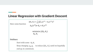
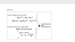
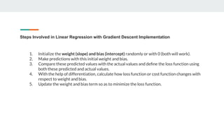
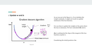
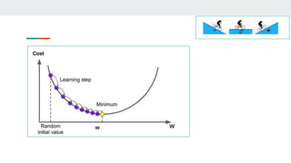
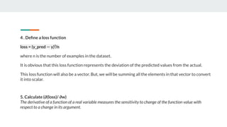
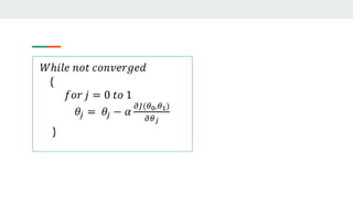
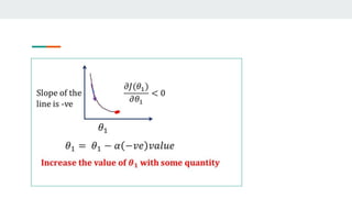
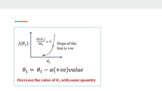
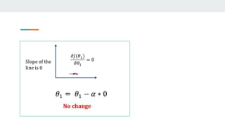
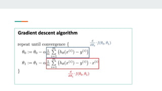
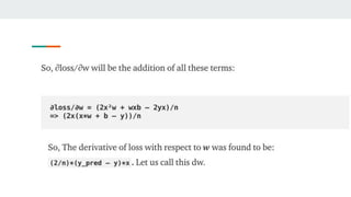
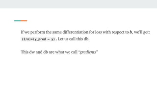
- Linear regression uses gradient descent to find the optimal weight (w) and bias (b) values that minimize the loss function and produce predictions closest to the actual target values. - It starts with random w and b values and calculates predictions. The loss function captures the deviation between predictions and targets. - It then computes the partial derivatives of the loss with respect to w and b to determine how to update them in a direction that decreases loss. 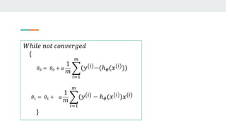- This process repeats in a training loop, updating w and b with each iteration until reaching a minimum loss, producing the optimal regression model.

1. Linear Regression with Gradient
Descent
Link to follow as per guidelines
https://medium.com/analytics-vidhya/linear-regression-with-gradient-descent-derivation-c10685ddf0f4
By: Sugandha Gupta

2. Understanding Gradient Descent Algorithm
Picture a scenario, you are playing a game with your friends where you have to throw a paper ball in a
basket. What will be your approach to this problem?
Here, I have a ball and basket at a particular distance, If I through the ball with 30% of my strength, I
believe it should end up in the basket. But with this force ball didn’t reach the target and falls before
the basket.

3. In my second attempt, I will use more power say 50% of my strength. This time I am sure it will reach
its place. But unexpectedly ball crosses the basket and falls far from it.

4. This time I threw the ball with 45% of my strength and yay! this time I succeed. The ball directly
drops in the basket. That means 45% of strength is the optimum solution for this problem.
This is how the gradient descent algorithm works.

5. Intuition to Gradient Descent

6. For a given problem statement, the solution starts with a Random initialization. These initial
parameters are then used to generate the predictions i.e the output.
Once we have the predicted values we can calculate the error or the cost. i.e how far the predicted
values are from the actual target.
In the next step, we update the parameters accordingly and again made the predictions with updated
parameters.
This process will go iteratively until we reach the optimum solution with minimal cost/error.

7. Gradient Descent
It is an optimization algorithm that works iteratively to find the model parameters with minimal cost
or error values.
It can be used to find the global or local minima of a differentiable function.

9. Linear Regression: Summary

10. Linear Regression with Gradient Descent

18. Notations used
Let’s say we have an independent variable x and a dependent variable y.
In order to form the relationship between these 2 variables, we have the equation:
y = x * w + b (same as y=mx + c )
where,
w is weight ( or slope ) ,
b is the bias (or intercept ),
x is the independent variable column vector(examples),
y is the dependent variable column vector(examples)

19. Our main goal is to find the w and b that defines the relationship between variable x and y correctly.
i.e. we want to find the line of regression that best fits the data.
We accomplish this with the help of something called as the Loss / Cost Function.
Loss Function: A loss function is a function that signifies how much our predicted values is deviated
from the actual values of the dependent variable.
Important Note: we are trying to find the values for w and b such that it minimizes our loss function.

20. Steps Involved in Linear Regression with Gradient Descent Implementation
1. Initialize the weight (slope) and bias (intercept) randomly or with 0 (both will work).
2. Make predictions with this initial weight and bias.
3. Compare these predicted values with the actual values and define the loss function using
both these predicted and actual values.
4. With the help of differentiation, calculate how loss function or cost function changes with
respect to weight and bias.
5. Update the weight and bias term so as to minimize the loss function.

21. Example X Y

22. 1 . Assumption
Let us say we have an x and y vectors like shown in the above pic (The above one is only for an example).
2. Initialize w and b to 0
w = 0, b = 0
3. Make some predictions with the current w and b. Of course, it’s going to be wrong.
y_pred = x*w + b, where y_pred stands for predicted y values.
This y_pred will also be a vector like y.

23. 4 . Define a loss function
loss = (y_pred — y)²/n
where n is the number of examples in the dataset.
It is obvious that this loss function represents the deviation of the predicted values from the actual.
This loss function will also be a vector. But, we will be summing all the elements in that vector to convert
it into scalar.
5. Calculate (∂(loss)/ ∂w)
The derivative of a function of a real variable measures the sensitivity to change of the function value with
respect to a change in its argument.

24. loss = (y_pred — y)²/n
loss = (y_pred² + y² — 2y*y_pred)/n (expanding the whole square)
=>( (x*w+b)² + y² — 2y*(x*w+b))/n (substitute y_pred)
=> ((x*w+b)²/n ) + (y²/n) + ((-2y(x*w+b))/n) (splitting the terms)
Let A = ((x*w+b)²/n ), B = (y²/n) and C = ((-2y(x*w+b))/n)

27. 6. Update w and b
As we can see in the figure 6.1, if we initialize the
weight randomly, it might not result in a global
minimum of the loss function.
It is our duty to update the weights to the point where
the loss is minimum. We have calculated dw above.
dw is nothing but the slope of the tangent of the loss
function at point w.
Considering the initial position of w.

28. Important points
● In the above diagram, The slope of the tangent of the loss will be positive as initial value of w
is greater and it needs to be reduced so as to attain global minimum.
● If the value of w is low and we want to increase it to attain global minimum, the slope of the
tangent of loss at point w will be negative.

29. We want the value of w to be a little lower so as to attain global minima of the loss function as shown in the figure 6.1.
We know that dw is positive in the above graph and we need to reduce w.
This can be done by:
w = w — alpha*dw
b = b — alpha*bw
where, alpha is a small number ranging between 0.1 to 0.0000001 (approx) and this alpha is known as the learning rate.
Doing this, we can reduce w if slope of tangent of loss at w is positive and increase w if slope is negative.

30. 7. Learning Rate
Learning rate alpha is something that we have to manually choose and it is something which we
don’t know beforehand. Choosing it is a matter of trial and error.
The reason we do not directly subtract dw from w is because, it might result in too much change
in the value of w and might not end up in global minimum but, even further away from it.

31. 8. Training Loop
The process of calculating the gradients and updating the weight and bias is repeated for
several times, which results in the optimized value for weight and bias.

32. 9. Prediction
After the training loop, the value of weight and bias is now optimized, which can be used
to predict new values given new x values.
y = x*w + b