1. 第16回 zansaの会
再発事象の解析をやってみる
@gepuro

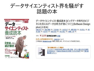
3. データサイエンティスト界を騒がす
話題の本

4. 発表前の様子

5. 発表後の様子
俺達もデータサイエンティストに!!

6. 本題に入ります。

7. 再発事象(recurrent events)とは
● 時間をかけて、何度も繰り返し発生するような事象
のことを言う。
● 例：がんの再発、ソフトウェアのバグが出る、クレー
ムが何度もあるetc

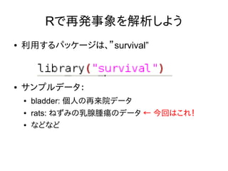
8. Rで再発事象を解析しよう
● 利用するパッケージは、”survival”
● サンプルデータ：
● bladder: 個人の再来院データ
● rats: ねずみの乳腺腫瘍のデータ ← 今回はこれ！
● などなど

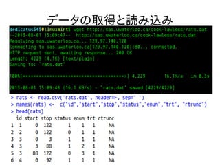
9. データの取得と読み込み

10. データの説明
● Id: ねずみの個体番号
● Start: 観測開始
● Stop: 観測終了
● Status: 1=腫瘍, 0=打ち切り
● Trt : 1=drug, 0=control
● ...

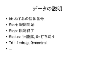
11. データの外観1
赤線はdrug、黒線はcontrolされているデータ
点は、腫瘍が発生した時点
時間
マウスid

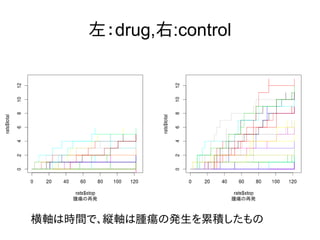
12. 左：drug,右:control
横軸は時間で、縦軸は腫瘍の発生を累積したもの

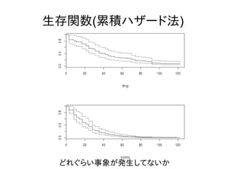
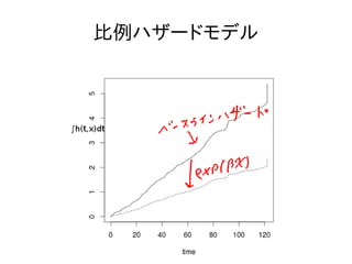
13. 生存関数(累積ハザード法)
どれぐらい事象が発生してないか

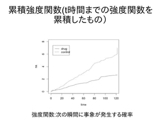
14. 累積強度関数(t時間までの強度関数を
累積したもの）
強度関数:次の瞬間に事象が発生する確率

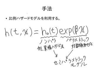
15. 手法
● 比例ハザードモデルを利用する。

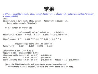
16. 結果

17. 比例ハザードモデル

19. 参考
● The Statistical Analysis of Recurrent Events
http://sas.uwaterloo.ca/cook-lawless/
● 講義ノートhttp://stat.inf.uec.ac.jp/dokuwiki/doku.php?
id=dm:2013
● 比例ハザードモデルはとってもtricky！
http://www.slideshare.net/takehikoihayashi/tricky
● 信頼性概論
http://avalonbreeze.web.fc2.com/38_01_02_reliability
outline.html

20. おまけ

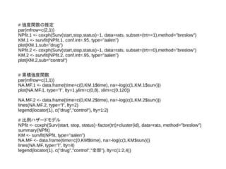
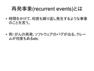
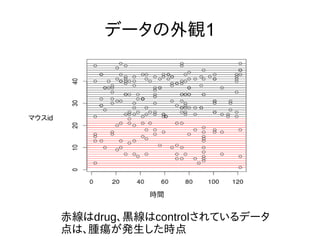
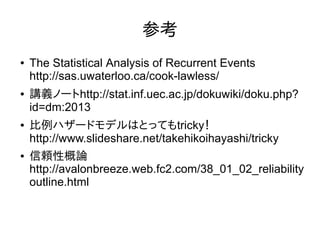
21. library("survival")
# wget http://sas.uwaterloo.ca/cook-lawless/rats.dat
rats <- read.csv("rats.dat", header=F, sep=" ")
names(rats) <- c("id","start","stop","status","enum","trt", "rtrunc")
head(rats)
rats$total <- NA
for(i in unique(rats$id)){
rats.id <- subset(rats, rats$id==i)
rats[which(rats$id==i),]$total <- cumsum(rats.id$status)
}
kaidan.plot <- function(rats){
plot(rats$stop, rats$total, xlim=c(0,125), ylim=c(0,13),sub="腫瘍の再発", type="n")
for(j in 1:nrow(rats)){
rats.j <- rats[j,]
segments(rats.j$start,rats.j$total-1, rats.j$stop, rats.j$total-1, col=rats.j$id)
segments(rats.j$stop, rats.j$total-1, rats.j$stop, rats.j$total, col=rats.j$id)
}
}
kaidan.plot(rats)
kaidan.plot(subset(rats, rats$trt==1))
kaidan.plot(subset(rats, rats$trt==0))
data.plot <- function(rats){
plot(seq(1,max(rats$stop),length.out=48),1:48, type="n",xlab="",ylab="")
abline(h=24:48)
abline(h=1:23,col="red")
rats.status1 <- subset(rats, rats$status==1)
points(rats.status1$stop, rats.status1$id)
}
data.plot(rats)

22. # 強度関数の推定
par(mfrow=c(2,1))
NPfit.1 <- coxph(Surv(start,stop,status)~1, data=rats, subset=(trt==1),method="breslow")
KM.1 <- survfit(NPfit.1, conf.int=.95, type="aalen")
plot(KM.1,sub="drug")
NPfit.2 <- coxph(Surv(start,stop,status)~1, data=rats, subset=(trt==0),method="breslow")
KM.2 <- survfit(NPfit.2, conf.int=.95, type="aalen")
plot(KM.2,sub="control")
# 累積強度関数
par(mfrow=c(1,1))
NA.MF.1 <- data.frame(time=c(0,KM.1$time), na=-log(c(1,KM.1$surv)))
plot(NA.MF.1, type="l", lty=1,ylim=c(0,8), xlim=c(0,120))
NA.MF.2 <- data.frame(time=c(0,KM.2$time), na=-log(c(1,KM.2$surv)))
lines(NA.MF.2, type="l", lty=2)
legend(locator(1), c("drug","control"), lty=1:2)
# 比例ハザードモデル
NPfit <- coxph(Surv(start, stop, status)~factor(trt)+cluster(id), data=rats, method="breslow")
summary(NPfit)
KM <- survfit(NPfit, type="aalen")
NA.MF <- data.frame(time=c(0,KM$time), na=-log(c(1,KM$surv)))
lines(NA.MF, type="l", lty=4)
legend(locator(1), c("drug","control","全部"), lty=c(1:2,4))