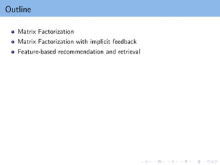
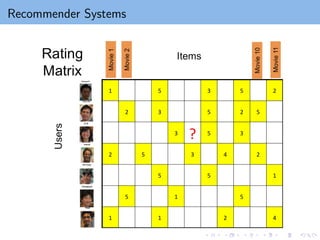
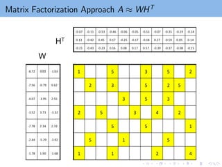
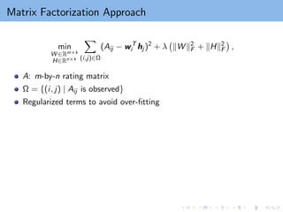
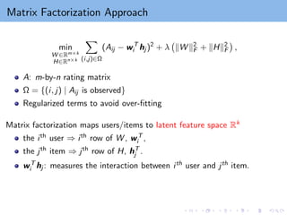
Matrix Factorization Approach
min
W∈Rm×k
H∈Rn×k
X
(i,j)∈Ω
(Aij − wT
i hj )2
+ λ kW k2
F + kHk2
F
,
A: m-by-n rating matrix
Ω = {(i, j) | Aij is observed}
Regularized terms to avoid over-fitting
7.
Matrix Factorization Approach
min
W∈Rm×k
H∈Rn×k
X
(i,j)∈Ω
(Aij − wT
i hj )2
+ λ kW k2
F + kHk2
F
,
A: m-by-n rating matrix
Ω = {(i, j) | Aij is observed}
Regularized terms to avoid over-fitting
Matrix factorization maps users/items to latent feature space Rk
the ith user ⇒ ith row of W , wT
i ,
the jth item ⇒ jth row of H, hT
j .
wT
i hj : measures the interaction between ith user and jth item.
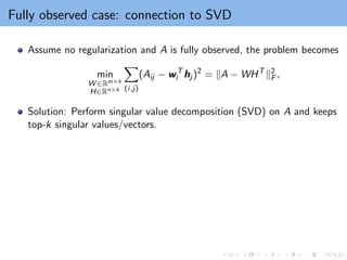
Fully observed case:connection to SVD
Assume no regularization and A is fully observed, the problem becomes
min
W ∈Rm×k
H∈Rn×k
X
(i,j)
(Aij − wT
i hj )2
= kA − WHT
k2
F ,
Solution: Perform singular value decomposition (SVD) on A and keeps
top-k singular values/vectors.
11.
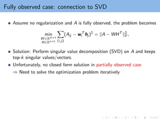
Fully observed case:connection to SVD
Assume no regularization and A is fully observed, the problem becomes
min
W ∈Rm×k
H∈Rn×k
X
(i,j)
(Aij − wT
i hj )2
= kA − WHT
k2
F ,
Solution: Perform singular value decomposition (SVD) on A and keeps
top-k singular values/vectors.
Unfortunately, no closed form solution in partially observed case
⇒ Need to solve the optimization problem iteratively
12.
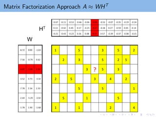
Properties of theObjective Function
Nonconvex problem
Example: f (x, y) = 1
2(xy − 1)2
∇f (0, 0) = 0, but clearly [0, 0] is not a global optimum
13.
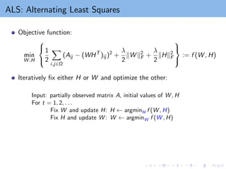
ALS: Alternating LeastSquares
Objective function:
min
W ,H
1
2
X
i,j∈Ω
(Aij − (WHT
)ij )2
+
λ
2
kW k2
F +
λ
2
kHk2
F
:= f (W , H)
Iteratively fix either H or W and optimize the other:
Input: partially observed matrix A, initial values of W , H
For t = 1, 2, . . .
Fix W and update H: H ← argminH f (W , H)
Fix H and update W : W ← argminW f (W , H)
14.
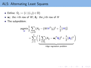
ALS: Alternating LeastSquares
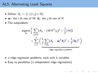
Define: Ωj := {i | (i, j) ∈ Ω}
wi : the i-th row of W ; hj : the j-th row of H
The subproblem:
argmin
H
1
2
X
i,j∈Ω
(Aij − (W HT
)ij )2
+
λ
2
kHk2
F
=
n
X
j=1
1
2
X
i∈Ωj
(Aij − wT
i hj )2
+
λ
2
khj k2
| {z }
ridge regression problem
15.
ALS: Alternating LeastSquares
Define: Ωj := {i | (i, j) ∈ Ω}
wi : the i-th row of W ; hj : the j-th row of H
The subproblem:
argmin
H
1
2
X
i,j∈Ω
(Aij − (W HT
)ij )2
+
λ
2
kHk2
F
=
n
X
j=1
1
2
X
i∈Ωj
(Aij − wT
i hj )2
+
λ
2
khj k2
| {z }
ridge regression problem
n ridge regression problems, each with k variables
Easy to parallelize (n independent ridge regressions)
16.
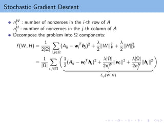
Stochastic Gradient Descent
nW
i: number of nonzeroes in the i-th row of A
nH
j : number of nonzeroes in the j-th column of A
Decompose the problem into Ω components:
f (W , H) =
1
2|Ω|
X
i,j∈Ω
(Aij − wT
i hj )2
+
λ
2
kW k2
F +
λ
2
kHk2
F
=
1
|Ω|
X
i,j∈Ω
1
2
(Aij − wT
i hj )2
+
λ|Ω|
2nW
i
kwi k2
+
λ|Ω|
2nH
j
khj k2
| {z }
fi,j (W ,H)
17.
Stochastic Gradient Descent
nW
i: number of nonzeroes in the i-th row of A
nH
j : number of nonzeroes in the j-th column of A
Decompose the problem into Ω components:
f (W , H) =
1
2|Ω|
X
i,j∈Ω
(Aij − wT
i hj )2
+
λ
2
kW k2
F +
λ
2
kHk2
F
=
1
|Ω|
X
i,j∈Ω
1
2
(Aij − wT
i hj )2
+
λ|Ω|
2nW
i
kwi k2
+
λ|Ω|
2nH
j
khj k2
| {z }
fi,j (W ,H)
The gradient of each component:
∇wi fi,j (W , H) = (wT
i hj − Aij )hj +
λ|Ω|
nW
i
wi
∇hj
fi,j (W , H) = (wT
i hj − Aij )wi +
λ|Ω|
nH
j
hj
18.
Stochastic Gradient Descent
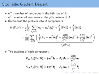
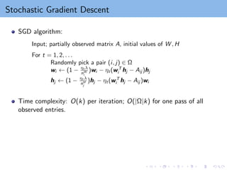
SGDalgorithm:
Input; partially observed matrix A, initial values of W , H
For t = 1, 2, . . .
Randomly pick a pair (i, j) ∈ Ω
wi ← (1 − ηt λ
nW
i
)wi − ηt(wT
i hj − Aij )hj
hj ← (1 − ηt λ
nH
j
)hj − ηt(wT
i hj − Aij )wi
19.
Stochastic Gradient Descent
SGDalgorithm:
Input; partially observed matrix A, initial values of W , H
For t = 1, 2, . . .
Randomly pick a pair (i, j) ∈ Ω
wi ← (1 − ηt λ
nW
i
)wi − ηt(wT
i hj − Aij )hj
hj ← (1 − ηt λ
nH
j
)hj − ηt(wT
i hj − Aij )wi
Time complexity: O(k) per iteration; O(|Ω|k) for one pass of all
observed entries.
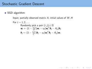
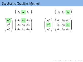
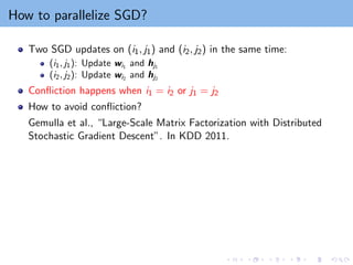
How to parallelizeSGD?
Two SGD updates on (i1, j1) and (i2, j2) in the same time:
(i1, j1): Update wi1
and hj1
(i2, j2): Update wi2
and hj2
Confliction happens when i1 = i2 or j1 = j2
How to avoid confliction?
Gemulla et al., “Large-Scale Matrix Factorization with Distributed
Stochastic Gradient Descent”. In KDD 2011.
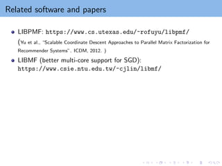
Related software andpapers
LIBPMF: https://www.cs.utexas.edu/~rofuyu/libpmf/
(Yu et al., “Scalable Coordinate Descent Approaches to Parallel Matrix Factorization for
Recommender Systems”. ICDM, 2012. )
LIBMF (better multi-core support for SGD):
https://www.csie.ntu.edu.tw/~cjlin/libmf/
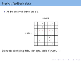
Implicit feedback data
Allthe observed entries are 1’s.
Examples: purchasing data, click data, social network, · · ·
28.
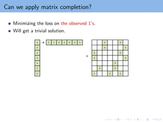
Can we applymatrix completion?
Minimizing the loss on the observed 1’s.
Will get a trivial solution.
29.
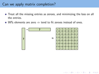
Can we applymatrix completion?
Treat all the missing entries as zeroes, and minimizing the loss on all
the entries.
99% elements are zero ⇒ tend to fit zeroes instead of ones.
30.
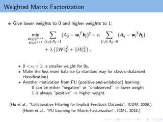
Weighted Matrix Factorization
Givelower weights to 0 and higher weights to 1:
min
W ∈Rm×k
H∈Rn×k
X
(i,j):Aij =1
(Aij − wT
i hj )2
+ α
X
(i,j):Aij =0
(Aij − wT
i hj )
+ λ kW k2
F + kHk2
F
,
0 α 1: a smaller weight for 0s.
Make the loss more balance (a standard way for class-unbalanced
classification)
Another motivation from PU (positive-and-unlabeled) learning:
0 can be either “negative” or “unobserved” ⇒ lower weight
1 is always “positive” ⇒ higher weight
(Hu et al., “Collaborative Filtering for Implicit Feedback Datasets”, ICDM, 2008.)
(Hsieh et al., “PU Learning for Matrix Factorization”, ICML, 2018.)
31.
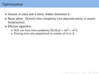
Optimization
Assume m usersand n items, hidden dimension k.
Naive solver: O(mnk) time complexity (mn observed entries in matrix
factorization)
Efficient algorithm:
ALS: can have time complexity O(kAk0k + mk2
+ nk2
).
Training time only proportional to number of 1s in A.
32.
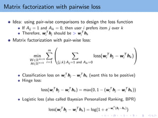
Matrix factorization withpairwise loss
Idea: using pair-wise comparisons to design the loss function
If Aij = 1 and Aik = 0, then user i prefers item j over k
Therefore, wT
i hj should be wT
i hk
Matrix factorization with pair-wise loss:
min
W ∈Rm×k
H∈Rn×k
m
X
i=1
X
(j,k):Aij =1 and Aik =0
loss(wT
i hj − wT
i hk)
Classification loss on wT
i hj − wT
i hk (want this to be positive)
Hinge loss:
loss(wT
i hj − wT
i hk ) = max(0, 1 − (wT
i hj − wT
i hk ))
Logistic loss (also called Bayesian Personalized Ranking, BPR)
loss(wT
i hj − wT
i hk ) = log(1 + e−wT
i (hj −hk )
)
33.
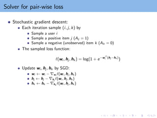
Solver for pair-wiseloss
Stochastic gradient descent:
Each iteration sample (i, j, k) by
Sample a user i
Sample a positive item j (Aij = 1)
Sample a negative (unobserved) item k (Aik = 0)
The sampled loss function:
`(wi , hj , hk ) = log(1 + e−wT
i (hj −hk )
)
Update wi , hj , hk by SGD:
wi ← wi − ∇wi `(wi , hj , hk )
hj ← hj − ∇hj
`(wi , hj , hk )
hk ← hk − ∇hk
`(wi , hj , hk )
34.
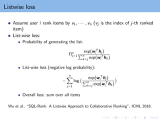
Listwise loss
Assume useri rank items by v1, · · · , vn (vj is the index of j-th ranked
item)
List-wise loss:
Probability of generating the list:
Πn
j=1
exp(wT
i hj )
Pn
k=j exp(wT
i hk )
List-wise loss (negative log probability):
−
n
X
j=1
log
exp(wT
i hj )
Pn
k=j exp(wT
i hk )
Overall loss: sum over all items
Wu et al., “SQL-Rank: A Listwise Approach to Collaborative Ranking”, ICML 2018.
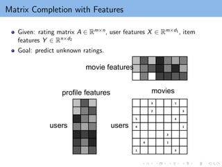
Inductive Matrix Completion(IMC)
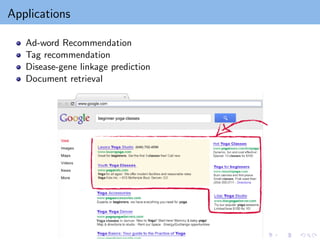
A popular approach to incorporate features to matrix completion.
Given row features X ∈ Rn1×d1 , column features Y ∈ Rn2×d2 ,
observation set Ω sampled from R, the IMC objective is:
min
W ∈Rd1×k
H∈Rd2×k
X
(i,j)∈Ω
(xT
i WHT
yj − Rij )2
+
λ
2
kW k2
F +
λ
2
kHk2
F
W xi : k-dimensional embedding of user i
Hyj : k-dimensional embedding of item j
Inner product in the k-dimensional embedding space ⇒ prediction value
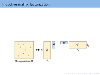
Factorization Machine
Widely usedfor recommender systems in companies and in data mining
competitions!
Proposed by (S. Rendle, “Factorization Machines”, in ICDM 2010. )
Observation: Recommendation systems can be transformed to
classification or regression
(i, j, Aij ) ⇒ (x(i,j)
, Aij ), where
x(i,j)
is the feature extracted for user i and item j
Example: x = [uT
i vT
j ], where ui is the feature for user i and vj is the
feature for user j
ui can include an indicator vector for user i and/or attributes of user i
Now we have a classification or regression problem with training data
{(x(i,j), Aij )}(i,j)∈Ω
Factorization Machine
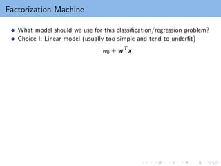
What modelshould we use for this classification/regression problem?
Choice I: Linear model (usually too simple and tend to underfit)
w0 + wT
x
44.
Factorization Machine
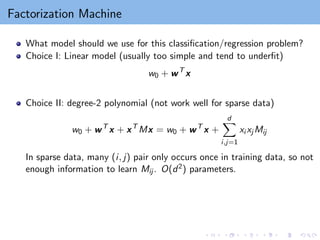
What modelshould we use for this classification/regression problem?
Choice I: Linear model (usually too simple and tend to underfit)
w0 + wT
x
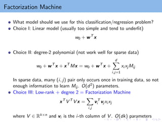
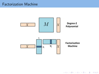
Choice II: degree-2 polynomial (not work well for sparse data)
w0 + wT
x + xT
Mx = w0 + wT
x +
d
X
i,j=1
xi xj Mij
In sparse data, many (i, j) pair only occurs once in training data, so not
enough information to learn Mij . O(d2) parameters.
45.
Factorization Machine
What modelshould we use for this classification/regression problem?
Choice I: Linear model (usually too simple and tend to underfit)
w0 + wT
x
Choice II: degree-2 polynomial (not work well for sparse data)
w0 + wT
x + xT
Mx = w0 + wT
x +
d
X
i,j=1
xi xj Mij
In sparse data, many (i, j) pair only occurs once in training data, so not
enough information to learn Mij . O(d2) parameters.
Choice III: Low-rank + degree 2 = Factorization Machine
xT
V T
V x =
X
i,j
vT
i vj xi xj
where V ∈ Rk×n and vi is the i-th column of V . O(dk) parameters
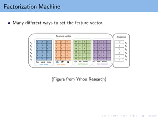
Factorization Machine: Training
Ω:observed entries, x(i,j): feature generated by i-th user and j-th item
(e.g, [uT
i vT
j ], where ui , vj are user/item features)
Solve the following minimization problem:
min
V ∈Rd×k
X
(i,j)∈Ω
loss(w0 + wT
x(i,j)
+ (x(i,j)
)T
VV T
x(i,j)
, Aij ) + λkV k2
F
LIBFM (by Steffen Rendle):
Alternating Minimization
SGD
Sampling
Is inductive matrix completion a special case of factorization machine?
48.
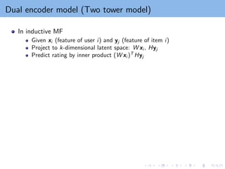
Dual encoder model(Two tower model)
In inductive MF
Given xi (feature of user i) and yj (feature of item i)
Project to k-dimensional latent space: W xi , Hyj
Predict rating by inner product (W xi )T
Hyj
49.
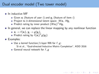
Dual encoder model(Two tower model)
In inductive MF
Given xi (feature of user i) and yj (feature of item i)
Project to k-dimensional latent space: W xi , Hyj
Predict rating by inner product (W xi )T
Hyj
In general, we can replace the linear mapping by any nonlinear function
xi → f (xi ), yj → g(yj ),
Predict rating by f (xi )T
g(yj )
Examples:
Use a kernel function/1-layer NN for f , g:
Si et al., “Goal-directed Inductive Matrix Completion”, KDD 2016
General neural network for f , g
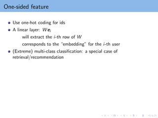
One-sided feature
Use one-hotcoding for ids
A linear layer: W ei
will extract the i-th row of W
corresponds to the “embedding” for the i-th user
(Extreme) multi-class classification: a special case of
retrieval/recommendation


![Properties of the Objective Function
Nonconvex problem
Example: f (x, y) = 1
2(xy − 1)2
∇f (0, 0) = 0, but clearly [0, 0] is not a global optimum](https://image.slidesharecdn.com/lecture13-260202185816-d84c985e/85/Lecture-13-Matrix-Factorization-and-Recommender-Systems-12-320.jpg)
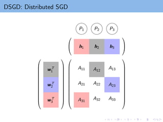
![DSGD: Distributed SGD [Gemulla et al, 2011]
wT
1
wT
2
wT
3
h1 h2 h3
A11
A12 A13
A21 A22
A23
A31 A32 A33
P1 P2 P3](https://image.slidesharecdn.com/lecture13-260202185816-d84c985e/85/Lecture-13-Matrix-Factorization-and-Recommender-Systems-22-320.jpg)


![Factorization Machine
Widely used for recommender systems in companies and in data mining
competitions!
Proposed by (S. Rendle, “Factorization Machines”, in ICDM 2010. )
Observation: Recommendation systems can be transformed to
classification or regression
(i, j, Aij ) ⇒ (x(i,j)
, Aij ), where
x(i,j)
is the feature extracted for user i and item j
Example: x = [uT
i vT
j ], where ui is the feature for user i and vj is the
feature for user j
ui can include an indicator vector for user i and/or attributes of user i
Now we have a classification or regression problem with training data
{(x(i,j), Aij )}(i,j)∈Ω](https://image.slidesharecdn.com/lecture13-260202185816-d84c985e/85/Lecture-13-Matrix-Factorization-and-Recommender-Systems-41-320.jpg)
![Factorization Machine: Training
Ω: observed entries, x(i,j): feature generated by i-th user and j-th item
(e.g, [uT
i vT
j ], where ui , vj are user/item features)
Solve the following minimization problem:
min
V ∈Rd×k
X
(i,j)∈Ω
loss(w0 + wT
x(i,j)
+ (x(i,j)
)T
VV T
x(i,j)
, Aij ) + λkV k2
F
LIBFM (by Steffen Rendle):
Alternating Minimization
SGD
Sampling
Is inductive matrix completion a special case of factorization machine?](https://image.slidesharecdn.com/lecture13-260202185816-d84c985e/85/Lecture-13-Matrix-Factorization-and-Recommender-Systems-47-320.jpg)