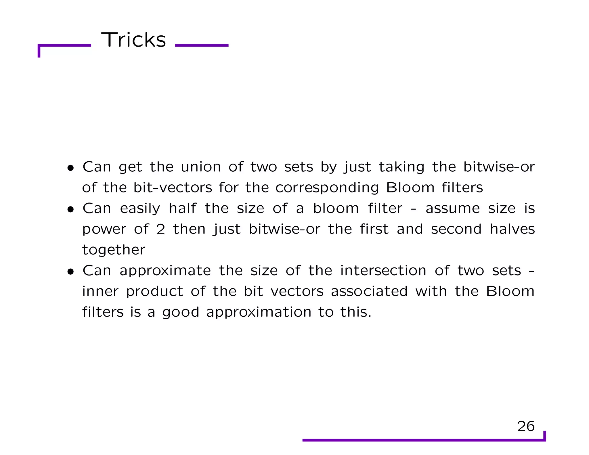
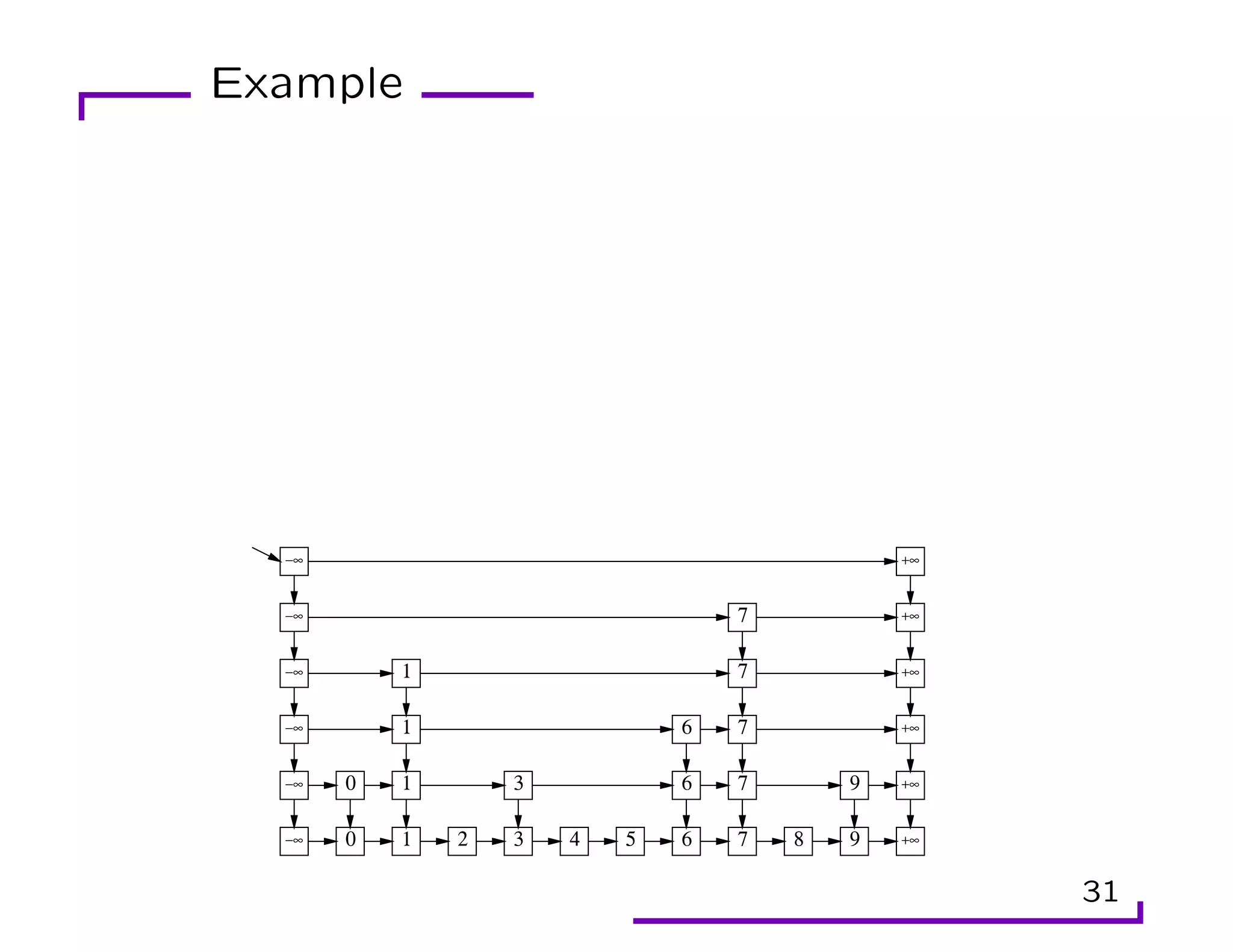
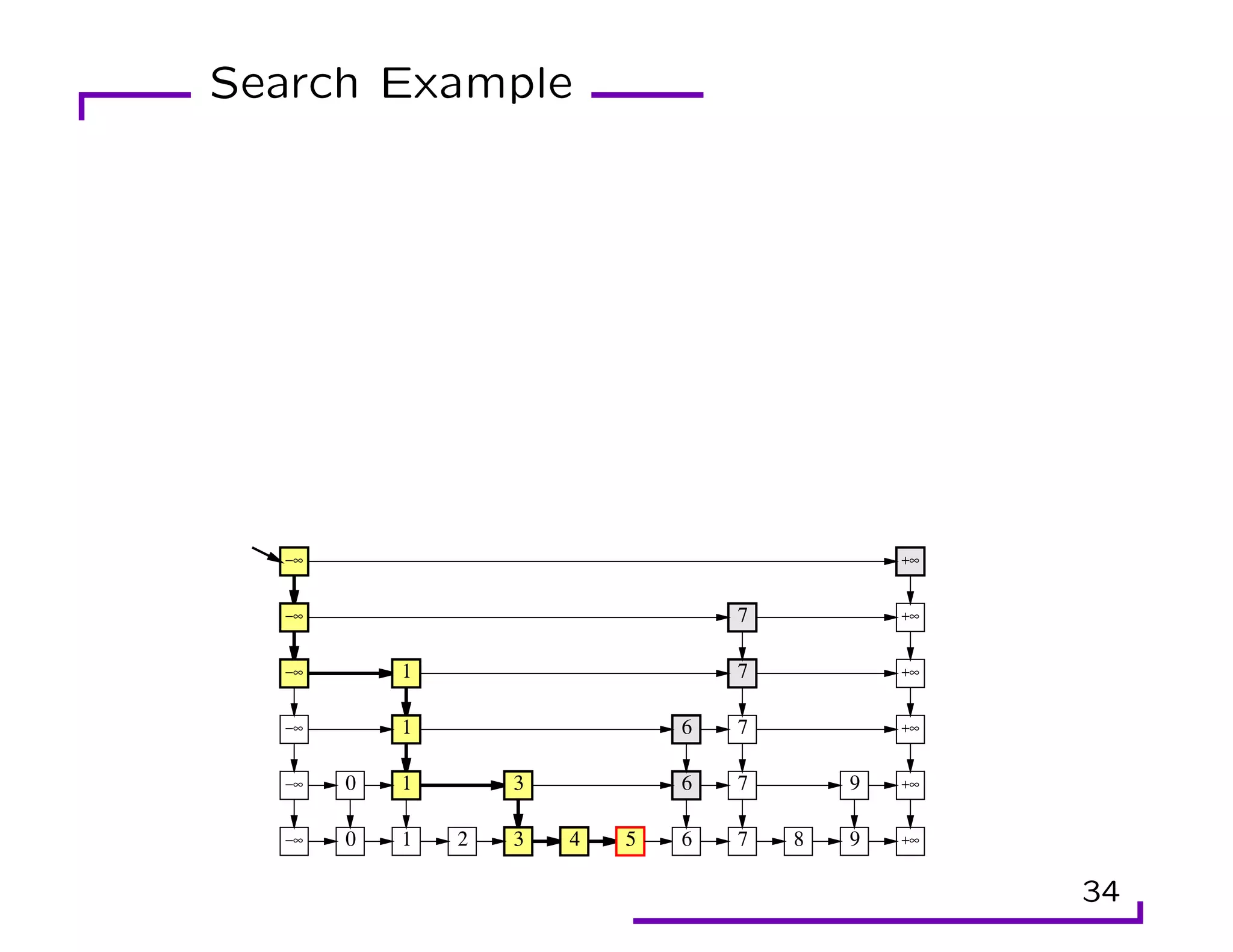
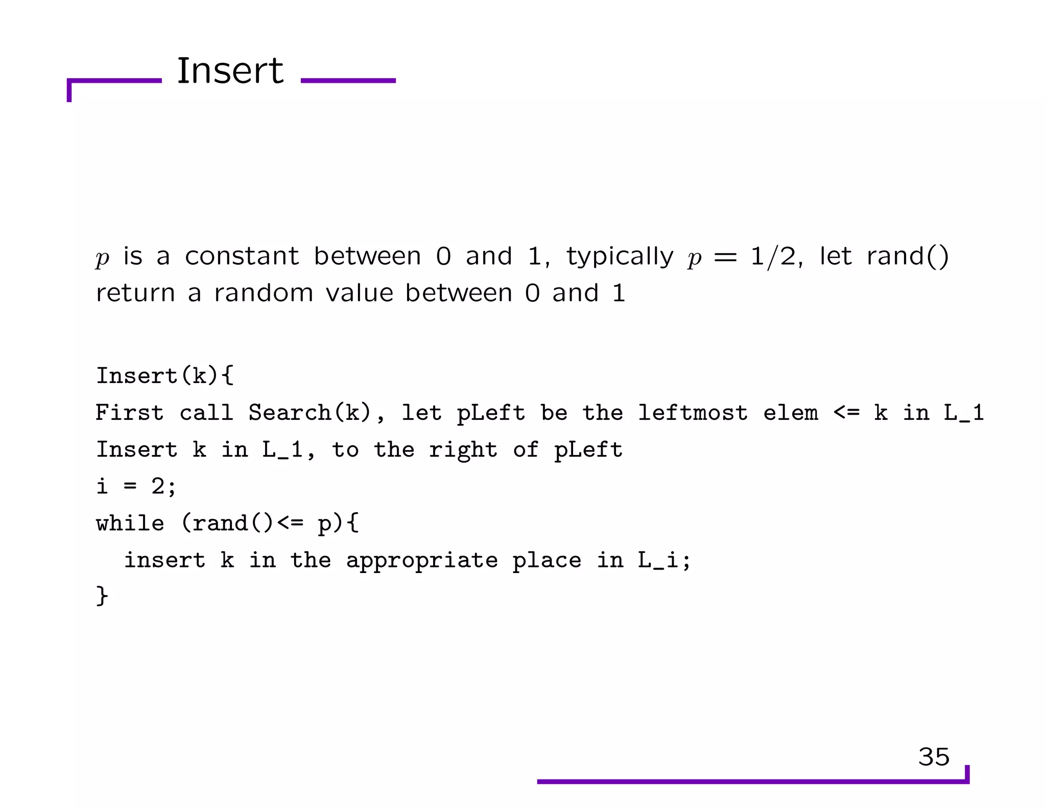
This document provides an overview of randomization techniques used in data structures, including hash tables, bloom filters, and skip lists. It discusses how each of these structures implements a dictionary abstract data type (ADT) with operations like insert, delete, and lookup. For hash tables, it describes direct addressing, chaining to resolve collisions, and analysis showing expected constant time performance. Bloom filters are explained as a space-efficient probabilistic data structure for set membership with possible false positives. Skip lists are randomized balanced search trees that provide logarithmic time performance for dictionary operations.

1. CS 561, Lecture 2 : Randomization in Data
Structures
Jared Saia
University of New Mexico

2. Outline
• Hash Tables
• Bloom Filters
• Skip Lists
1

3. Dictionary ADT
A dictionary ADT implements the following operations
• Insert(x): puts the item x into the dictionary
• Delete(x): deletes the item x from the dictionary
• IsIn(x): returns true iff the item x is in the dictionary
2

4. Dictionary ADT
• Frequently, we think of the items being stored in the dictio-
nary as keys
• The keys typically have records associated with them which
are carried around with the key but not used by the ADT
implementation
• Thus we can implement functions like:
– Insert(k,r): puts the item (k,r) into the dictionary if the
key k is not already there, otherwise returns an error
– Delete(k): deletes the item with key k from the dictionary
– Lookup(k): returns the item (k,r) if k is in the dictionary,
otherwise returns null
3

5. Implementing Dictionaries
• The simplest way to implement a dictionary ADT is with a
linked list
• Let l be a linked list data structure, assume we have the
following operations defined for l
– head(l): returns a pointer to the head of the list
– next(p): given a pointer p into the list, returns a pointer
to the next element in the list if such exists, null otherwise
– previous(p): given a pointer p into the list, returns a
pointer to the previous element in the list if such exists,
null otherwise
– key(p): given a pointer into the list, returns the key value
of that item
– record(p): given a pointer into the list, returns the record
value of that item
4

6. At-Home Exercise
Implement a dictionary with a linked list
• Q1: Write the operation Lookup(k) which returns a pointer
to the item with key k if it is in the dictionary or null otherwise
• Q2: Write the operation Insert(k,r)
• Q3: Write the operation Delete(k)
• Q4: For a dictionary with n elements, what is the runtime
of all of these operations for the linked list data structure?
• Q5: Describe how you would use this dictionary ADT to
count the number of occurences of each word in an online
book.
5

7. Dictionaries
• This linked list implementation of dictionaries is very slow
• Q: Can we do better?
• A: Yes, with hash tables, AVL trees, etc
6

8. Hash Tables
Hash Tables implement the Dictionary ADT, namely:
• Insert(x) - O(1) expected time, Θ(n) worst case
• Lookup(x) - O(1) expected time, Θ(n) worst case
• Delete(x) - O(1) expected time, Θ(n) worst case
7

9. Direct Addressing
• Suppose universe of keys is U = {0, 1, . . . , m − 1}, where m is
not too large
• Assume no two elements have the same key
• We use an array T[0..m − 1] to store the keys
• Slot k contains the elem with key k
8

10. Direct Address Functions
DA-Search(T,k){ return T[k];}
DA-Insert(T,x){ T[key(x)] = x;}
DA-Delete(T,x){ T[key(x)] = NIL;}
Each of these operations takes O(1) time
9

11. Direct Addressing Problem
• If universe U is large, storing the array T may be impractical
• Also much space can be wasted in T if number of objects
stored is small
• Q: Can we do better?
• A: Yes we can trade time for space
10

12. Hash Tables
• “Key” Idea: An element with key k is stored in slot h(k),
where h is a hash function mapping U into the set {0, . . . , m−
1}
• Main problem: Two keys can now hash to the same slot
• Q: How do we resolve this problem?
• A1: Try to prevent it by hashing keys to “random” slots and
making the table large enough
• A2: Chaining
• A3: Open Addressing
11

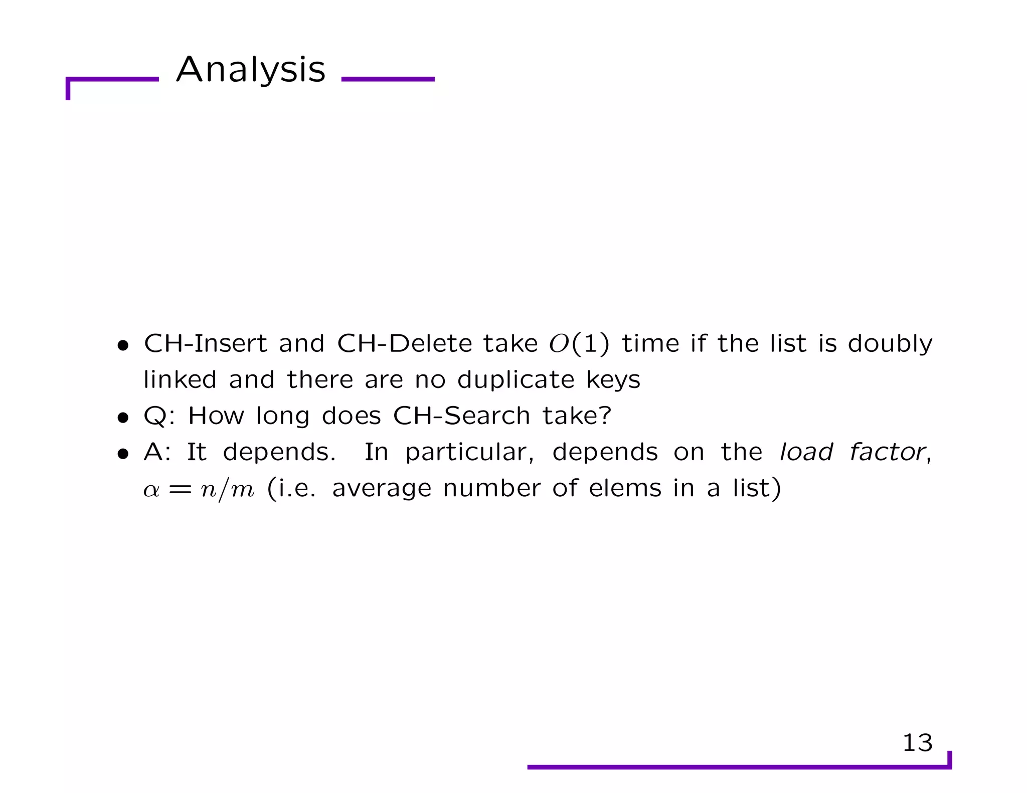
13. Chained Hash
In chaining, all elements that hash to the same slot are put in a
linked list.
CH-Insert(T,x){Insert x at the head of list T[h(key(x))];}
CH-Search(T,k){search for elem with key k in list T[h(k)];}
CH-Delete(T,x){delete x from the list T[h(key(x))];}
12

14. Analysis
• CH-Insert and CH-Delete take O(1) time if the list is doubly
linked and there are no duplicate keys
• Q: How long does CH-Search take?
• A: It depends. In particular, depends on the load factor,
α = n/m (i.e. average number of elems in a list)
13

15. CH-Search Analysis
• Worst case analysis: everyone hashes to one slot so Θ(n)
• For average case, make the simple uniform hashing assump-
tion: any given elem is equally likely to hash into any of the
m slots, indep. of the other elems
• Let ni be a random variable giving the length of the list at
the i-th slot
• Then time to do a search for key k is 1 + nh(k)
14

16. CH-Search Analysis
• Q: What is E(nh(k))?
• A: We know that h(k) is uniformly distributed among {0, .., m−
1}
• Thus, E(nh(k)) =
Pm−1
i=0 (1/m)ni = n/m = α
15

17. Hash Functions
• Want each key to be equally likely to hash to any of the m
slots, independently of the other keys
• Key idea is to use the hash function to “break up” any pat-
terns that might exist in the data
• We will always assume a key is a natural number (can e.g.
easily convert strings to naturaly numbers)
16

18. Division Method
• h(k) = k mod m
• Want m to be a prime number, which is not too close to a
power of 2
• Why? Reduces collisions in the case where there is periodicity
in the keys inserted
17

19. Hash Tables Wrapup
Hash Tables implement the Dictionary ADT, namely:
• Insert(x) - O(1) expected time, Θ(n) worst case
• Lookup(x) - O(1) expected time, Θ(n) worst case
• Delete(x) - O(1) expected time, Θ(n) worst case
18

20. Bloom Filters
• Randomized data structure for representing a set. Imple-
ments:
• Insert(x) :
• IsMember(x) :
• Allow false positives but require very little space
• Used frequently in: Databases, networking problems, p2p
networks, packet routing
19

21. Bloom Filters
• Have m slots, k hash functions, n elements; assume hash
functions are all independent
• Each slot stores 1 bit, initially all bits are 0
• Insert(x) : Set the bit in slots h1(x), h2(x), ..., hk(x) to 1
• IsMember(x) : Return yes iff the bits in h1(x), h2(x), ..., hk(x)
are all 1
20

22. Analysis Sketch
• m slots, k hash functions, n elements; assume hash functions
are all independent
• Then P(fixed slot is still 0) = (1 − 1/m)kn
• Useful fact from Taylor expansion of e−x:
e−x − x2/2 ≤ 1 − x ≤ e−x for x < 1
• Then if x ≤ 1
e−x(1 − x2) ≤ 1 − x ≤ e−x
21

23. Analysis
• Thus we have the following to good approximation.
P(fixed slot is still 0) = (1 − 1/m)kn
≈ e−km/n
• Let p = e−kn/m and let ρ be the fraction of 0 bits after n
elements inserted then
P(false positive) = (1 − ρ)k ≈ (1 − p)k
• Where the first approximation holds because ρ is very close
to p (by a Martingale argument beyond the scope of this
class)
22

24. Analysis
• Want to minimize (1−p)k, which is equivalent to minimizing
g = k ln(1 − p)
• Trick: Note that g = −(n/m) ln(p) ln(1 − p)
• By symmetry, this is minimized when p = 1/2 or equivalently
k = (m/n) ln 2
• False positive rate is then (1/2)k ≈ (.6185)m/n
23

25. Tricks
• Can get the union of two sets by just taking the bitwise-or
of the bit-vectors for the corresponding Bloom filters
• Can easily half the size of a bloom filter - assume size is
power of 2 then just bitwise-or the first and second halves
together
• Can approximate the size of the intersection of two sets -
inner product of the bit vectors associated with the Bloom
filters is a good approximation to this.
26

26. Extensions
• Counting Bloom filters handle deletions: instead of storing
bits, store integers in the slots. Insertion increments, deletion
decrements.
• Bloomier Filters: Also allow for data to be inserted in the
filter - similar functionality to hash tables but less space, and
the possibility of false positives.
27

27. Skip List
• Enables insertions and searches for ordered keys in O(log n)
expected time
• Very elegant randomized data structure, simple to code but
analysis is subtle
• They guarantee that, with high probability, all the major op-
erations take O(log n) time (e.g. Find-Max, Find i-th ele-
ment, etc.)
28

28. Skip List
• A skip list is basically a collection of doubly-linked lists,
L1, L2, . . . , Lx, for some integer x
• Each list has a special head and tail node, the keys of these
nodes are assumed to be −MAXNUM and +MAXNUM re-
spectively
• The keys in each list are in sorted order (non-decreasing)
29

29. Skip List
• Every node is stored in the bottom list
• For each node in the bottom list, we flip a coin over and
over until we get tails. For each heads, we make a duplicate
of the node.
• The duplicates are stacked up in levels and the nodes on
each level are strung together in sorted linked lists
• Each node v stores a search key (key(v)), a pointer to its
next lower copy (down(v)), and a pointer to the next node
in its level (right(v)).
30

30. Example
−∞ +∞
−∞ +∞
−∞ +∞
−∞ +∞
−∞ +∞
−∞ +∞
1 2 3 4 5 6 7 8 9
0
1 6 7 9
0
1 6 7
3
1 7
7
31

31. Search
• To do a search for a key, x, we start at the leftmost node L
in the highest level
• We then scan through each level as far as we can without
passing the target value x and then proceed down to the next
level
• The search ends either when we find the key x or fail to find
x on the lowest level
32

32. Search
SkipListFind(x, L){
v = L;
while (v != NULL) and (Key(v) != x){
if (Key(Right(v)) > x)
v = Down(v);
else
v = Right(v);
}
return v;
}
33

33. Search Example
−∞ +∞
1 2 3 4 5 6 7 8 9
0
−∞ +∞
1 6 7 9
0
−∞ +∞
1 6 7
3
−∞ +∞
1 7
−∞ +∞
7
−∞ +∞
34

34. Insert
p is a constant between 0 and 1, typically p = 1/2, let rand()
return a random value between 0 and 1
Insert(k){
First call Search(k), let pLeft be the leftmost elem <= k in L_1
Insert k in L_1, to the right of pLeft
i = 2;
while (rand()<= p){
insert k in the appropriate place in L_i;
}
35

35. Deletion
• Deletion is very simple
• First do a search for the key to be deleted
• Then delete that key from all the lists it appears in from
the bottom up, making sure to “zip up” the lists after the
deletion
36

36. Analysis
• Intuitively, each level of the skip list has about half the num-
ber of nodes of the previous level, so we expect the total
number of levels to be about O(log n)
• Similarly, each time we add another level, we cut the search
time in half except for a constant overhead
• So after O(log n) levels, we would expect a search time of
O(log n)
• We will now formalize these two intuitive observations
37

37. Height of Skip List
• For some key, i, let Xi be the maximum height of i in the
skip list.
• Q: What is the probability that Xi ≥ 2 log n?
• A: If p = 1/2, we have:
P(Xi ≥ 2 log n) =
1
2
2 log n
=
1
(2log n)2
=
1
n2
• Thus the probability that a particular key i achieves height
2 log n is 1
n2
38

38. Height of Skip List
• Q: What is the probability that any key achieves height
2 log n?
• A: We want
P(X1 ≥ 2 log n or X2 ≥ 2 log n or . . . or Xn ≥ 2 log n)
• By a Union Bound, this probability is no more than
P(X1 ≥ k log n) + P(X2 ≥ k log n) + · · · + P(Xn ≥ k log n)
• Which equals:
n
X
i=1
1
n2
=
n
n2
= 1/n
39

39. Height of Skip List
• This probability gets small as n gets large
• In particular, the probability of having a skip list of size ex-
ceeding 2 log n is o(1)
• If an event occurs with probability 1 − o(1), we say that it
occurs with high probability
• Key Point: The height of a skip list is O(log n) with high
probability.
40

40. In-Class Exercise Trick
A trick for computing expectations of discrete positive random
variables:
• Let X be a discrete r.v., that takes on values from 1 to n
E(X) =
n
X
i=1
P(X ≥ i)
41

41. Why?
n
X
i=1
P(X ≥ i) = P(X = 1) + P(X = 2) + P(X = 3) + . . .
+ P(X = 2) + P(X = 3) + P(X = 4) + . . .
+ P(X = 3) + P(X = 4) + P(X = 5) + . . .
+ . . .
= 1 ∗ P(X = 1) + 2 ∗ P(X = 2) + 3 ∗ P(X = 3) + . . .
= E(X)
42

42. In-Class Exercise
Q: How much memory do we expect a skip list to use up?
• Let Xi be the number of lists that element i is inserted in.
• Q: What is P(Xi ≥ 1), P(Xi ≥ 2), P(Xi ≥ 3)?
• Q: What is P(Xi ≥ k) for general k?
• Q: What is E(Xi)?
• Q: Let X =
Pn
i=1 Xi. What is E(X)?
43

43. Search Time
• Its easier to analyze the search time if we imagine running
the search backwards
• Imagine that we start at the found node v in the bottommost
list and we trace the path backwards to the top leftmost
senitel, L
• This will give us the length of the search path from L to v
which is the time required to do the search
44

44. Backwards Search
SLFback(v){
while (v != L){
if (Up(v)!=NIL)
v = Up(v);
else
v = Left(v);
}}
45

45. Backward Search
• For every node v in the skip list Up(v) exists with probability
1/2. So for purposes of analysis, SLFBack is the same as
the following algorithm:
FlipWalk(v){
while (v != L){
if (COINFLIP == HEADS)
v = Up(v);
else
v = Left(v);
}}
46

46. Analysis
• For this algorithm, the expected number of heads is exactly
the same as the expected number of tails
• Thus the expected run time of the algorithm is twice the
expected number of upward jumps
• Since we already know that the number of upward jumps
is O(log n) with high probability, we can conclude that the
expected search time is O(log n)
47