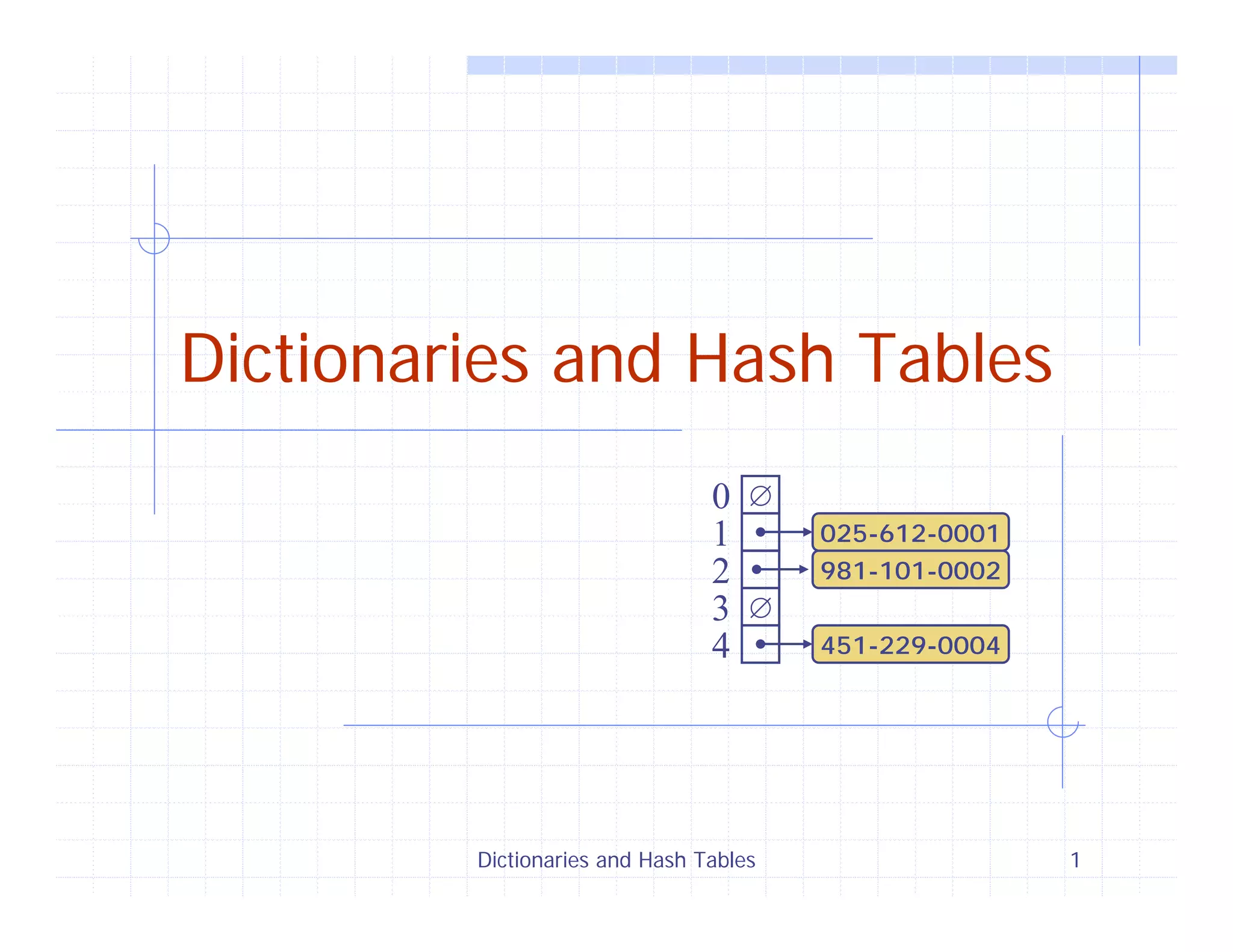
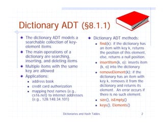
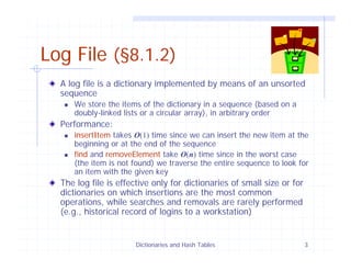
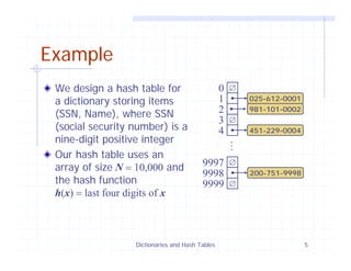
Dictionaries and hash tables are data structures for storing and searching key-value pairs. A dictionary abstract data type (ADT) allows searching, inserting, and deleting items by key. A log file dictionary implements the ADT using an unsorted sequence, with O(1) insertion but O(n) search and removal. A hash table maps keys to array indices using a hash function for expected O(1) operations, handling collisions by chaining or probing. Common hash functions include modular arithmetic and polynomial evaluation.

1. Dictionaries and Hash Tables 1
Dictionaries and Hash Tables
∅
∅
0
1
2
3
4 451-229-0004
981-101-0002
025-612-0001

2. Dictionaries and Hash Tables 2
Dictionary ADT (§8.1.1)
The dictionary ADT models a
searchable collection of key-
element items
The main operations of a
dictionary are searching,
inserting, and deleting items
Multiple items with the same
key are allowed
Applications:
address book
credit card authorization
mapping host names (e.g.,
cs16.net) to internet addresses
(e.g., 128.148.34.101)
Dictionary ADT methods:
find(k): if the dictionary has
an item with key k, returns
the position of this element,
else, returns a null position.
insertItem(k, o): inserts item
(k, o) into the dictionary
removeElement(k): if the
dictionary has an item with
key k, removes it from the
dictionary and returns its
element. An error occurs if
there is no such element.
size(), isEmpty()
keys(), Elements()

3. Dictionaries and Hash Tables 3
Log File (§8.1.2)
A log file is a dictionary implemented by means of an unsorted
sequence
We store the items of the dictionary in a sequence (based on a
doubly-linked lists or a circular array), in arbitrary order
Performance:
insertItem takes O(1) time since we can insert the new item at the
beginning or at the end of the sequence
find and removeElement take O(n) time since in the worst case
(the item is not found) we traverse the entire sequence to look for
an item with the given key
The log file is effective only for dictionaries of small size or for
dictionaries on which insertions are the most common
operations, while searches and removals are rarely performed
(e.g., historical record of logins to a workstation)

4. Dictionaries and Hash Tables 4
Hash Functions and
Hash Tables (§8.2)
A hash function h maps keys of a given type to
integers in a fixed interval [0, N − 1]
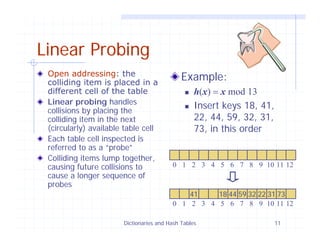
Example:
h(x) = x mod N
is a hash function for integer keys
The integer h(x) is called the hash value of key x
A hash table for a given key type consists of
Hash function h
Array (called table) of size N
When implementing a dictionary with a hash table,
the goal is to store item (k, o) at index i = h(k)

5. Dictionaries and Hash Tables 5
Example
We design a hash table for
a dictionary storing items
(SSN, Name), where SSN
(social security number) is a
nine-digit positive integer
Our hash table uses an
array of size N = 10,000 and
the hash function
h(x) = last four digits of x
∅
∅
∅
∅
0
1
2
3
4
9997
9998
9999
…
451-229-0004
981-101-0002
200-751-9998
025-612-0001

6. Dictionaries and Hash Tables 6
Hash Functions (§8.2.2)
A hash function is usually
specified as the composition
of two functions:
Hash code map:
h1: keys → integers
Compression map:
h2: integers → [0, N − 1]
The hash code map is
applied first, and the
compression map is
applied next on the
result, i.e.,
h(x) = h2(h1(x))
The goal of the hash
function is to
“disperse” the keys as
uniformly as possible

7. Dictionaries and Hash Tables 7
Hash Code Maps (§8.2.3)
Memory address:
Reinterpret the memory
address of the key object as
an integer
Integer cast:
We reinterpret the bits of the
key as an integer
Suitable for keys of length
less than or equal to the
number of bits of the integer
type (e.g., char, short, int
and float on many machines)
Component sum:
We partition the bits of
the key into components
of fixed length (e.g., 16
or 32 bits) and we sum
the components
(ignoring overflows)
Suitable for numeric keys
of fixed length greater
than or equal to the
number of bits of the
integer type (e.g., long
and double on many
machines)

8. Dictionaries and Hash Tables 8
Hash Code Maps (cont.)
Polynomial accumulation:
We partition the bits of the
key into a sequence of
components of fixed length
(e.g., 8, 16 or 32 bits)
a0 a1 … an−1
We evaluate the polynomial
p(z) = a0 + a1 z + a2 z2 + …
… + an−1zn−1
at a fixed value z, ignoring
overflows
Especially suitable for strings
(e.g., the choice z = 33 gives
at most 6 collisions on a set
of 50,000 English words)
Polynomial p(z) can be
evaluated in O(n) time
using Horner’s rule:
The following
polynomials are
successively computed,
each from the previous
one in O(1) time
p0(z) = an−1
pi (z) = an−i−1 + zpi−1(z)
(i = 1, 2, …, n −1)
We have p(z) = pn−1(z)

9. Dictionaries and Hash Tables 9
Compression
Maps (§8.2.4)
Division:
h2 (y) = y mod N
The size N of the
hash table is usually
chosen to be a prime
Multiply, Add and
Divide (MAD):
h2 (y) = (ay + b) mod N
a and b are
nonnegative integers
such that
a mod N ≠ 0
Otherwise, every
integer would map to
the same value b

10. Dictionaries and Hash Tables 10
Collision Handling
(§8.2.5)
Collisions occur when
different elements are
mapped to the same
cell
Chaining: let each
cell in the table point
to a linked list of
elements that map
there
Chaining is simple,
but requires
additional memory
outside the table
∅
∅
∅
0
1
2
3
4 451-229-0004 981-101-0004
025-612-0001

11. Dictionaries and Hash Tables 11
Linear Probing
Open addressing: the
colliding item is placed in a
different cell of the table
Linear probing handles
collisions by placing the
colliding item in the next
(circularly) available table cell
Each table cell inspected is
referred to as a “probe”
Colliding items lump together,
causing future collisions to
cause a longer sequence of
probes
Example:
h(x) = x mod 13
Insert keys 18, 41,
22, 44, 59, 32, 31,
73, in this order
0 1 2 3 4 5 6 7 8 9 10 11 12
41 18 44 59 32 22 31 73
0 1 2 3 4 5 6 7 8 9 10 11 12

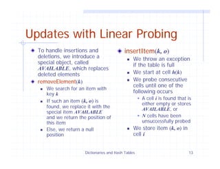
12. Dictionaries and Hash Tables 12
Search with Linear Probing
Consider a hash table A
that uses linear probing
find(k)
We start at cell h(k)
We probe consecutive
locations until one of the
following occurs
An item with key k is
found, or
An empty cell is found,
or
N cells have been
unsuccessfully probed
Algorithm find(k)
i ← h(k)
p ← 0
repeat
c ← A[i]
if c = ∅
return Position(null)
else if c.key () = k
return Position(c)
else
i ← (i + 1) mod N
p ← p + 1
until p = N
return Position(null)

13. Dictionaries and Hash Tables 13
Updates with Linear Probing
To handle insertions and
deletions, we introduce a
special object, called
AVAILABLE, which replaces
deleted elements
removeElement(k)
We search for an item with
key k
If such an item (k, o) is
found, we replace it with the
special item AVAILABLE
and we return the position of
this item
Else, we return a null
position
insertItem(k, o)
We throw an exception
if the table is full
We start at cell h(k)
We probe consecutive
cells until one of the
following occurs
A cell i is found that is
either empty or stores
AVAILABLE, or
N cells have been
unsuccessfully probed
We store item (k, o) in
cell i

14. Dictionaries and Hash Tables 14
Double Hashing
Double hashing uses a
secondary hash function
d(k) and handles
collisions by placing an
item in the first available
cell of the series
(i + jd(k)) mod N
for j = 0, 1, … , N − 1
The secondary hash
function d(k) cannot
have zero values
The table size N must be
a prime to allow probing
of all the cells
Common choice of
compression map for the
secondary hash function:
d2(k) = q − k mod q
where
q < N
q is a prime
The possible values for
d2(k) are
1, 2, … , q

15. Dictionaries and Hash Tables 15
Consider a hash
table storing integer
keys that handles
collision with double
hashing
N = 13, q = 7
h(k) = k mod 13
d(k) = 7 − k mod 7
(h(k) + jd(k)) mod N
j = 0, 1, …
Insert keys 18, 41,
22, 44, 59, 32, 31,
73, in this order
Example of Double Hashing
0 1 2 3 4 5 6 7 8 9 10 11 12
31 41 18 32 59 73 22 44
0 1 2 3 4 5 6 7 8 9 10 11 12
k h (k ) d (k ) Probes
18 5 3 5
41 2 1 2
22 9 6 9
44 5 5 5 10
59 7 4 7
32 6 3 6
31 5 4 5 9 0
73 8 4 8

16. Dictionaries and Hash Tables 16
Performance of
Hashing
In the worst case, searches,
insertions and removals on a
hash table take O(n) time
The worst case occurs when
all the keys inserted into the
dictionary collide
The load factor α = n/N
affects the performance of a
hash table
Assuming that the keys are
random numbers, it can be
shown that the expected
number of probes for an
insertion with open
addressing is
1 / (1 − α)
The expected running
time of all the dictionary
ADT operations in a
hash table is O(1)
In practice, hashing is
very fast provided the
load factor is not close
to 100%
Applications of hash
tables:
small databases
compilers
browser caches