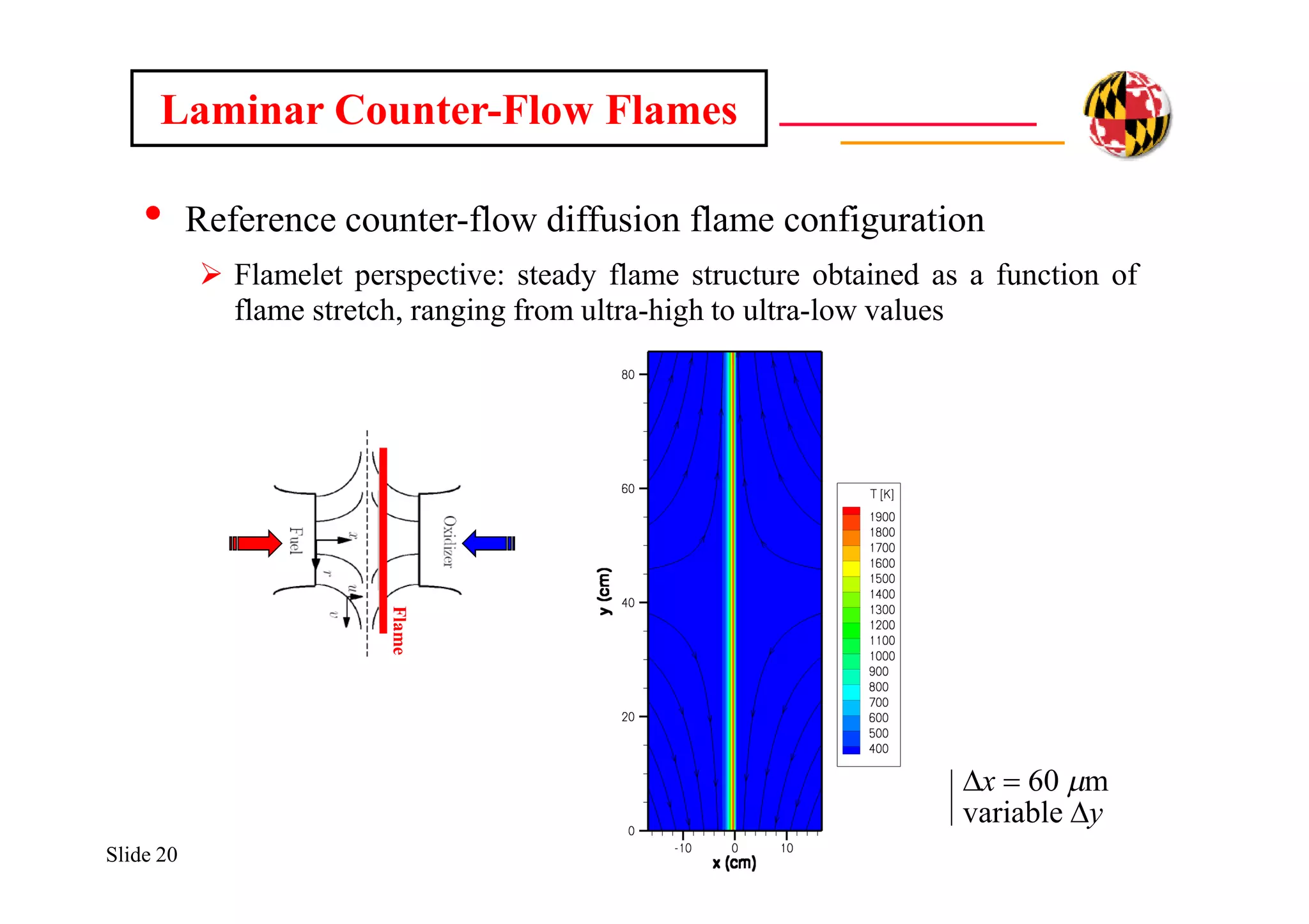
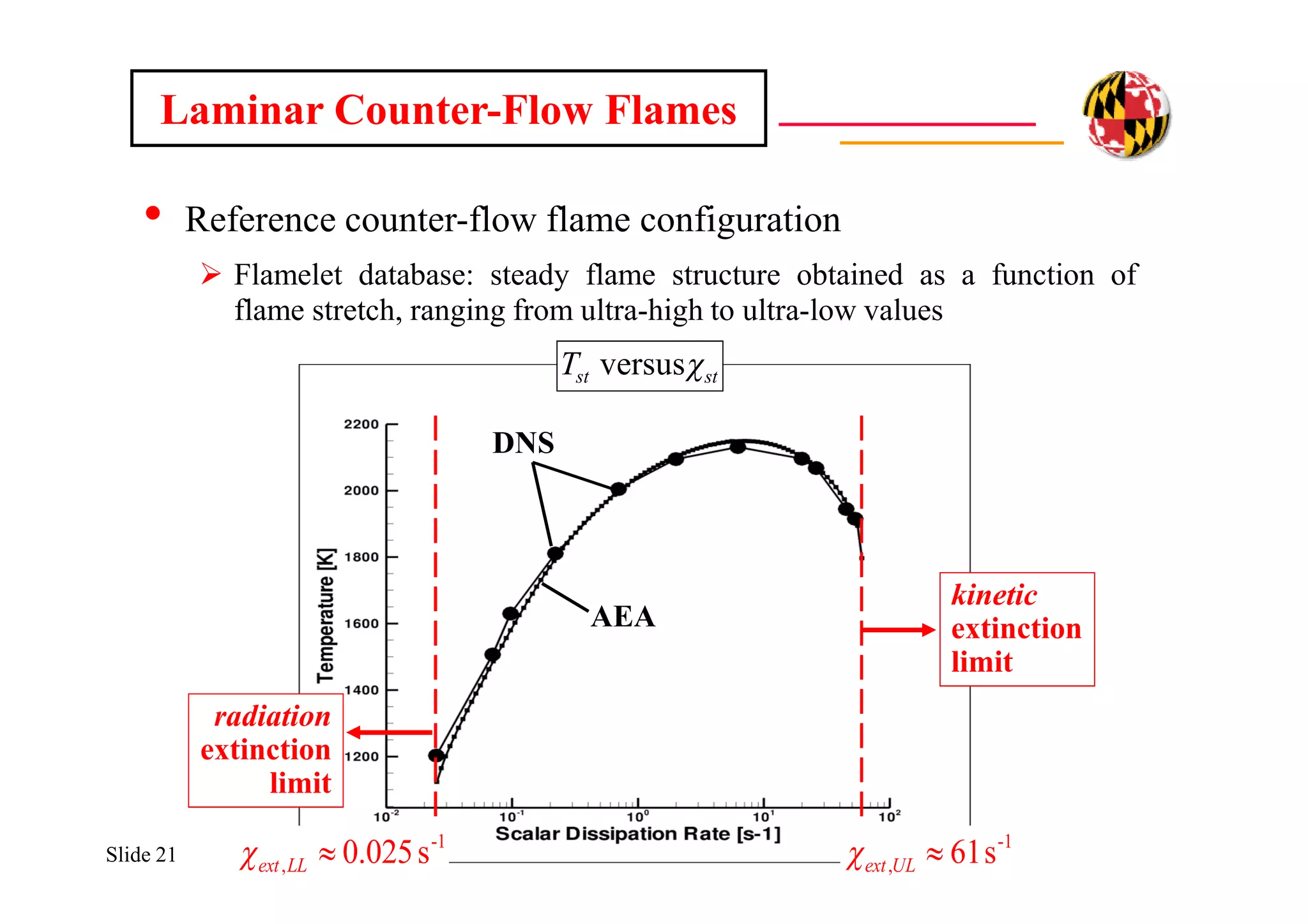
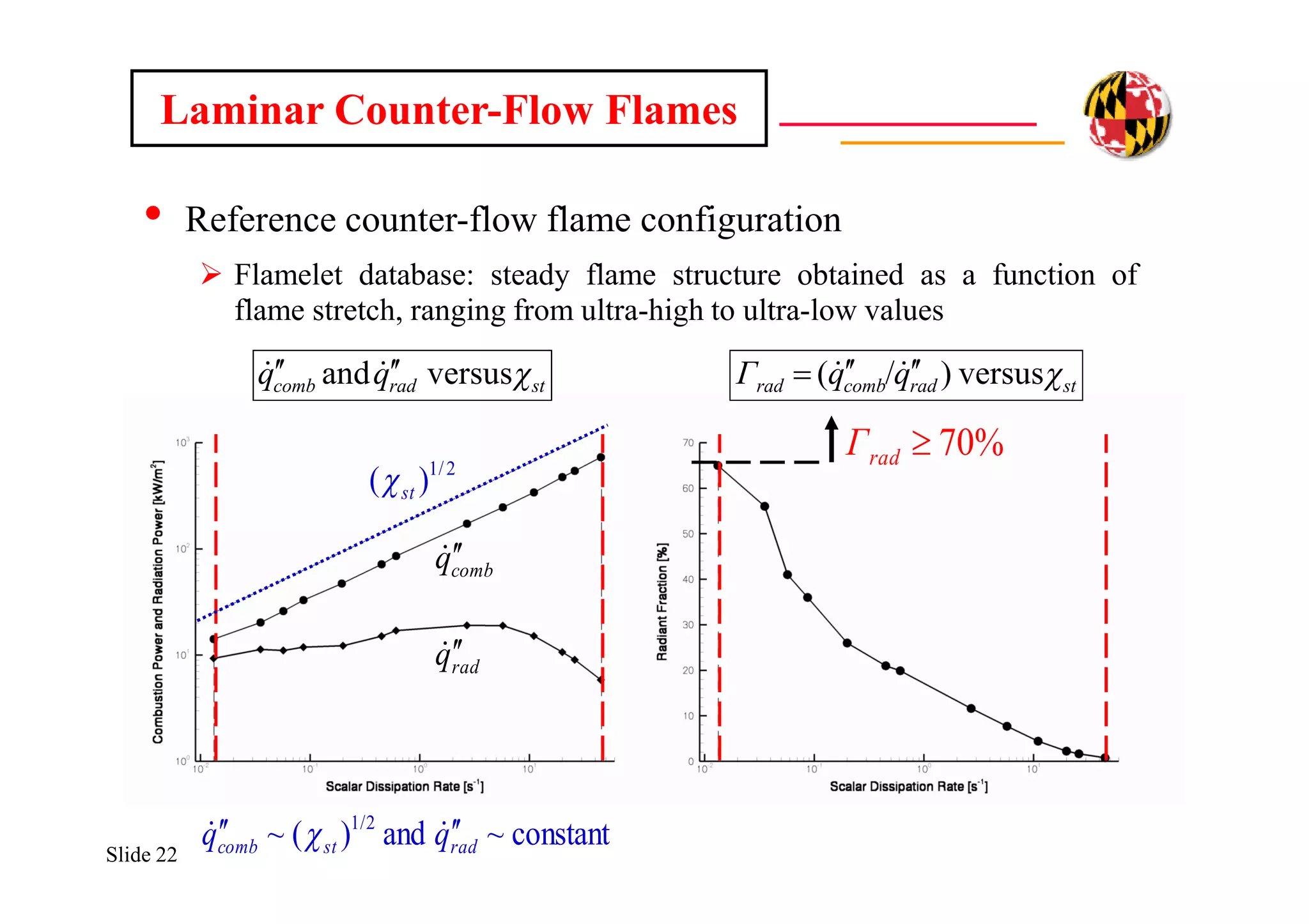
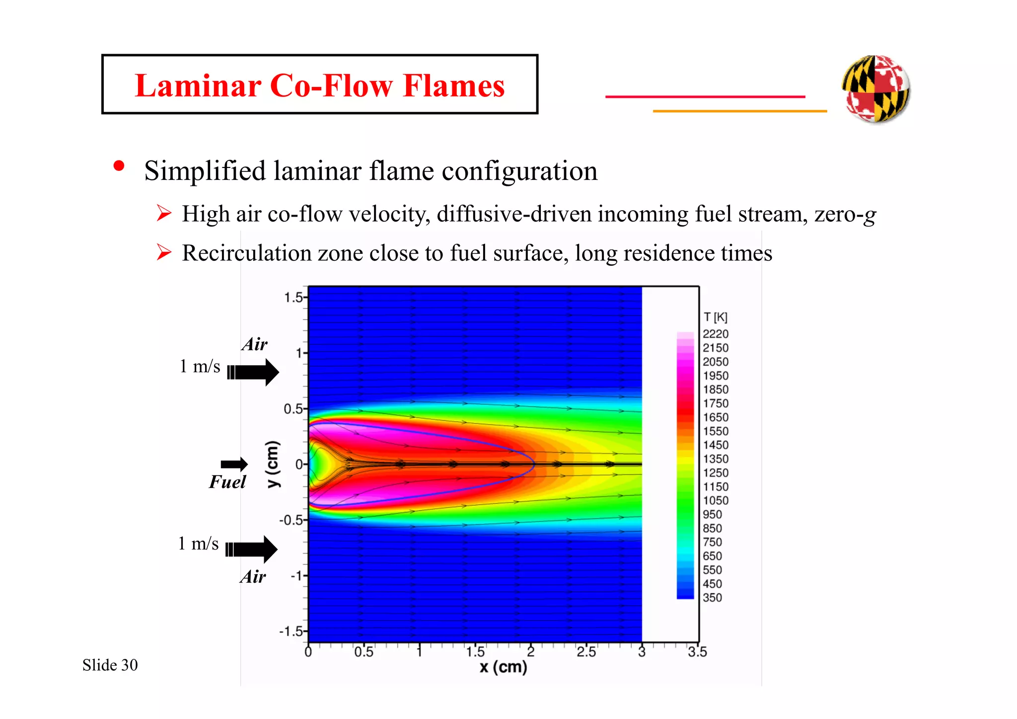
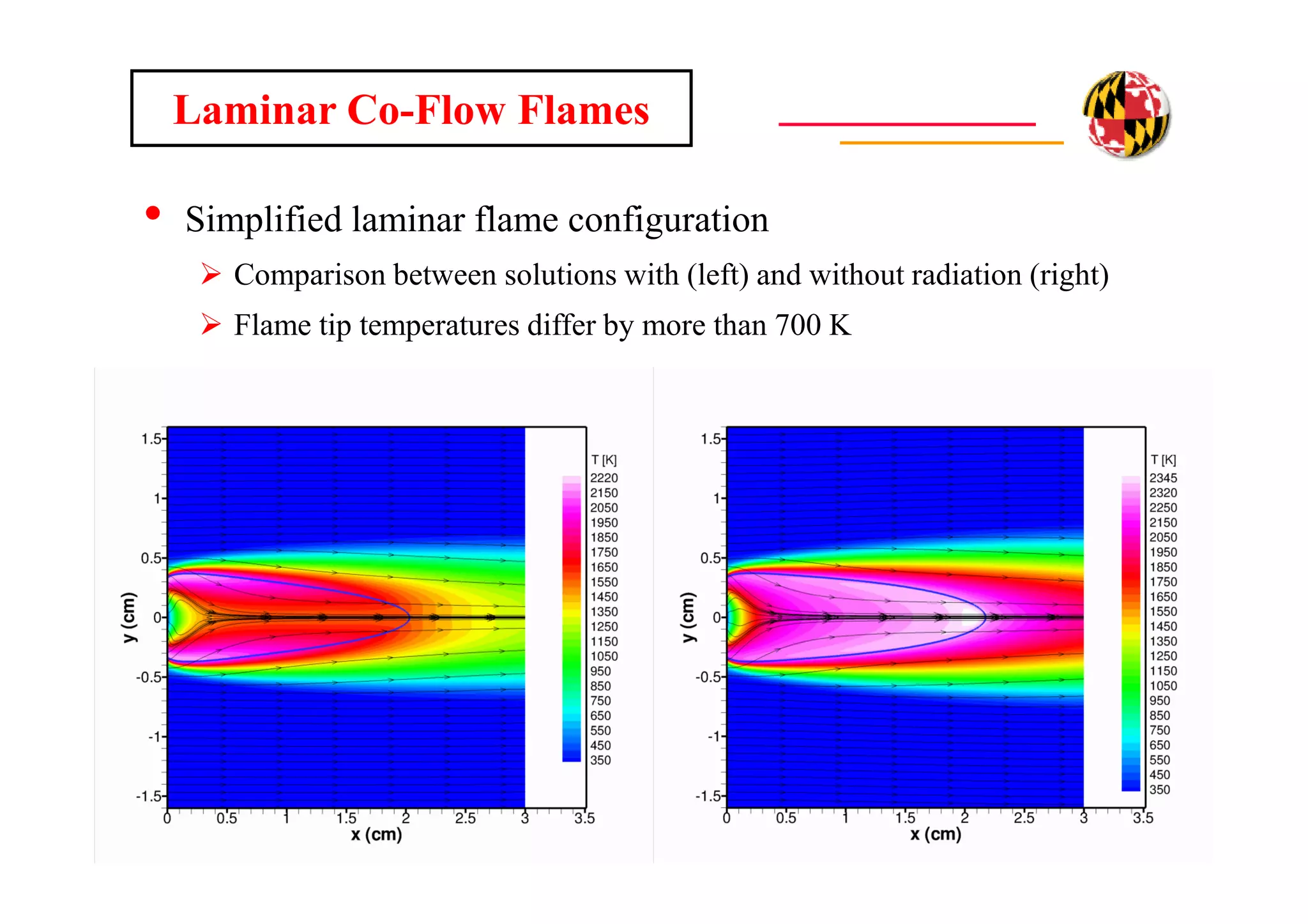
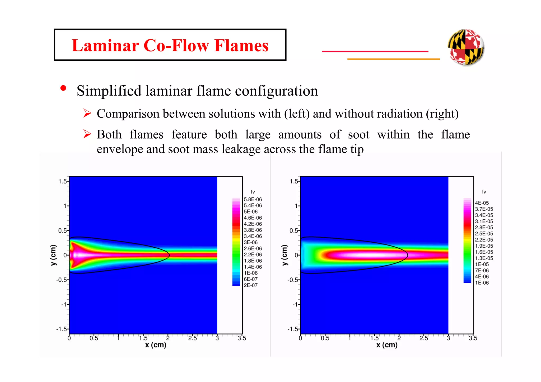
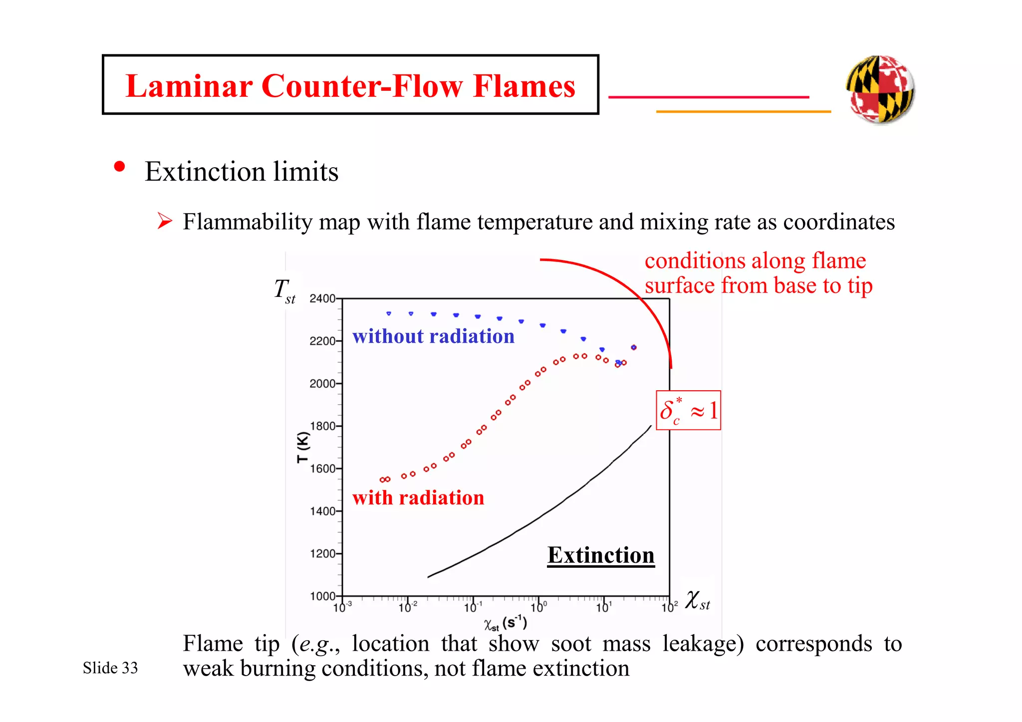
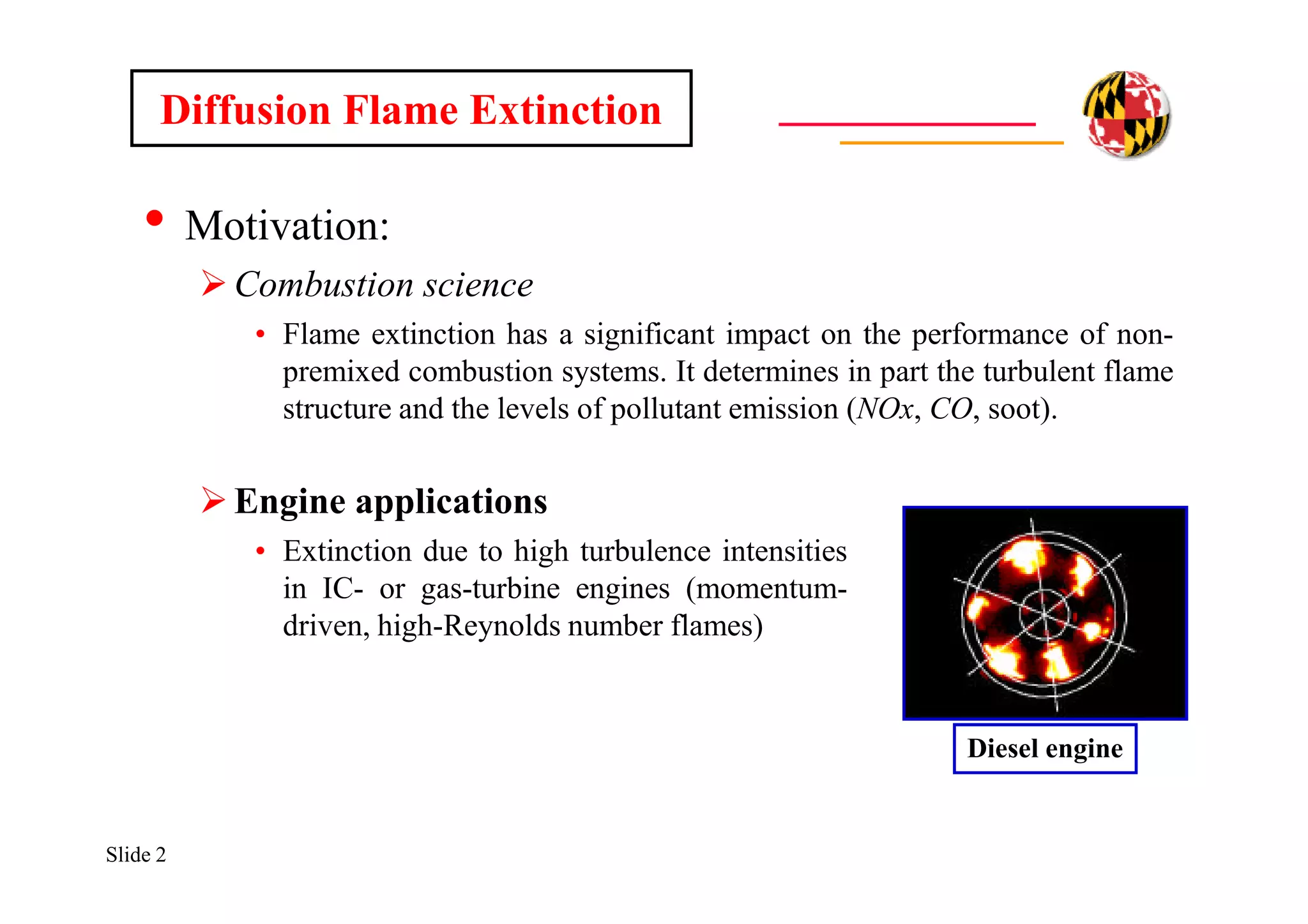
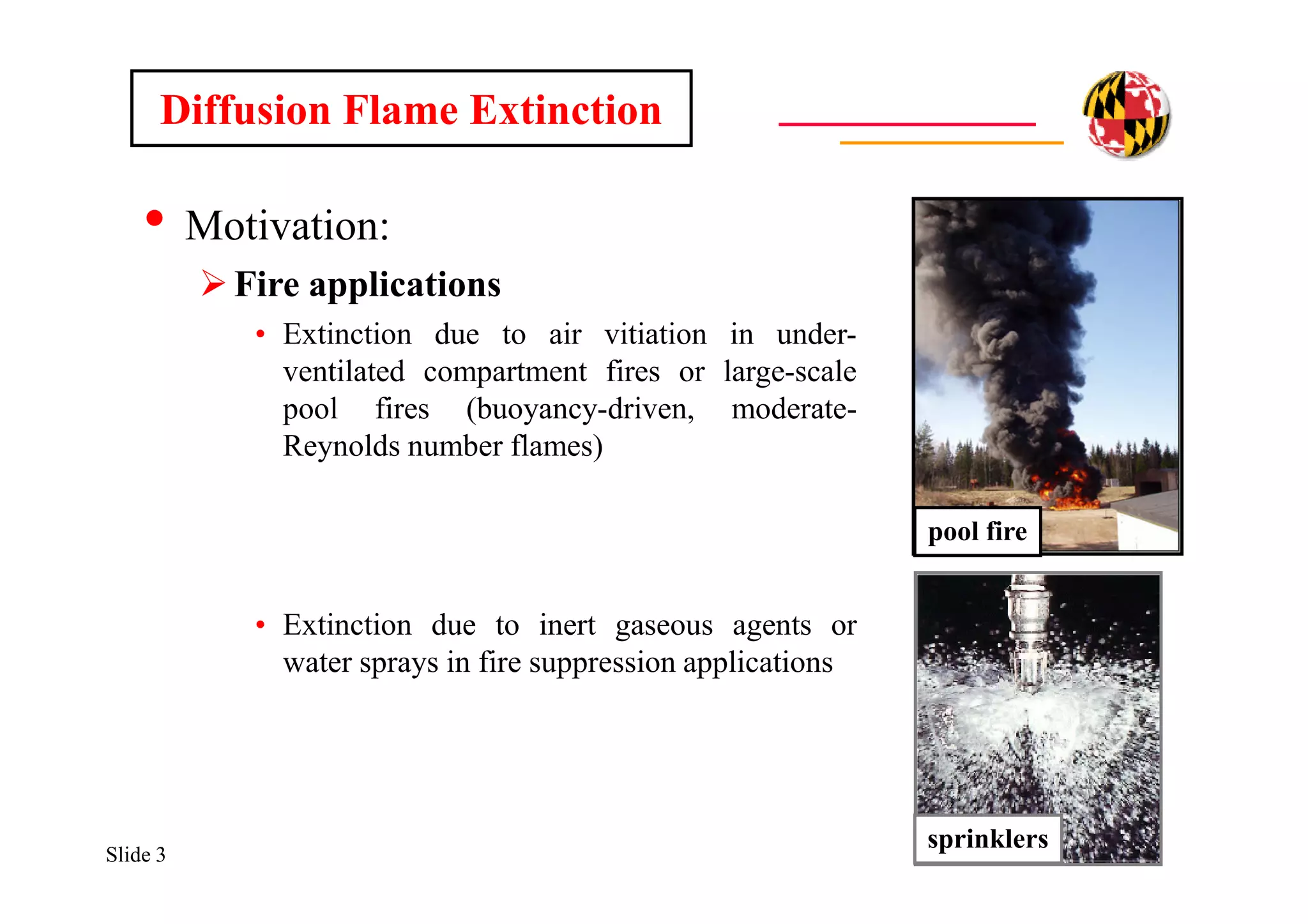
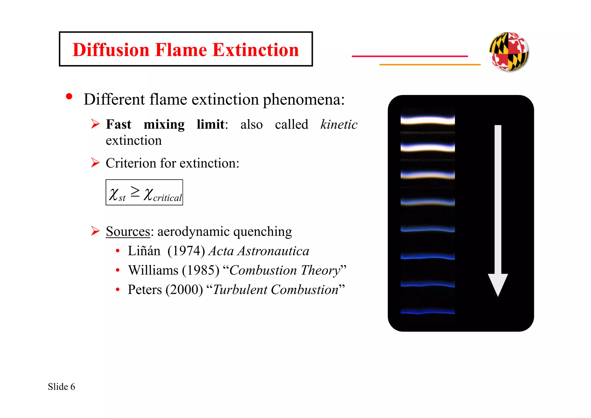
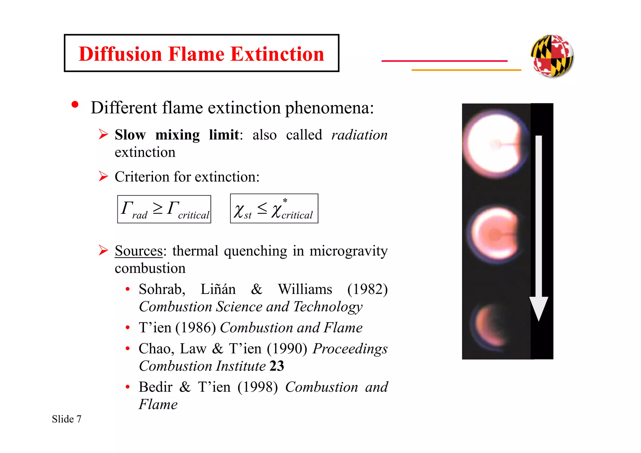
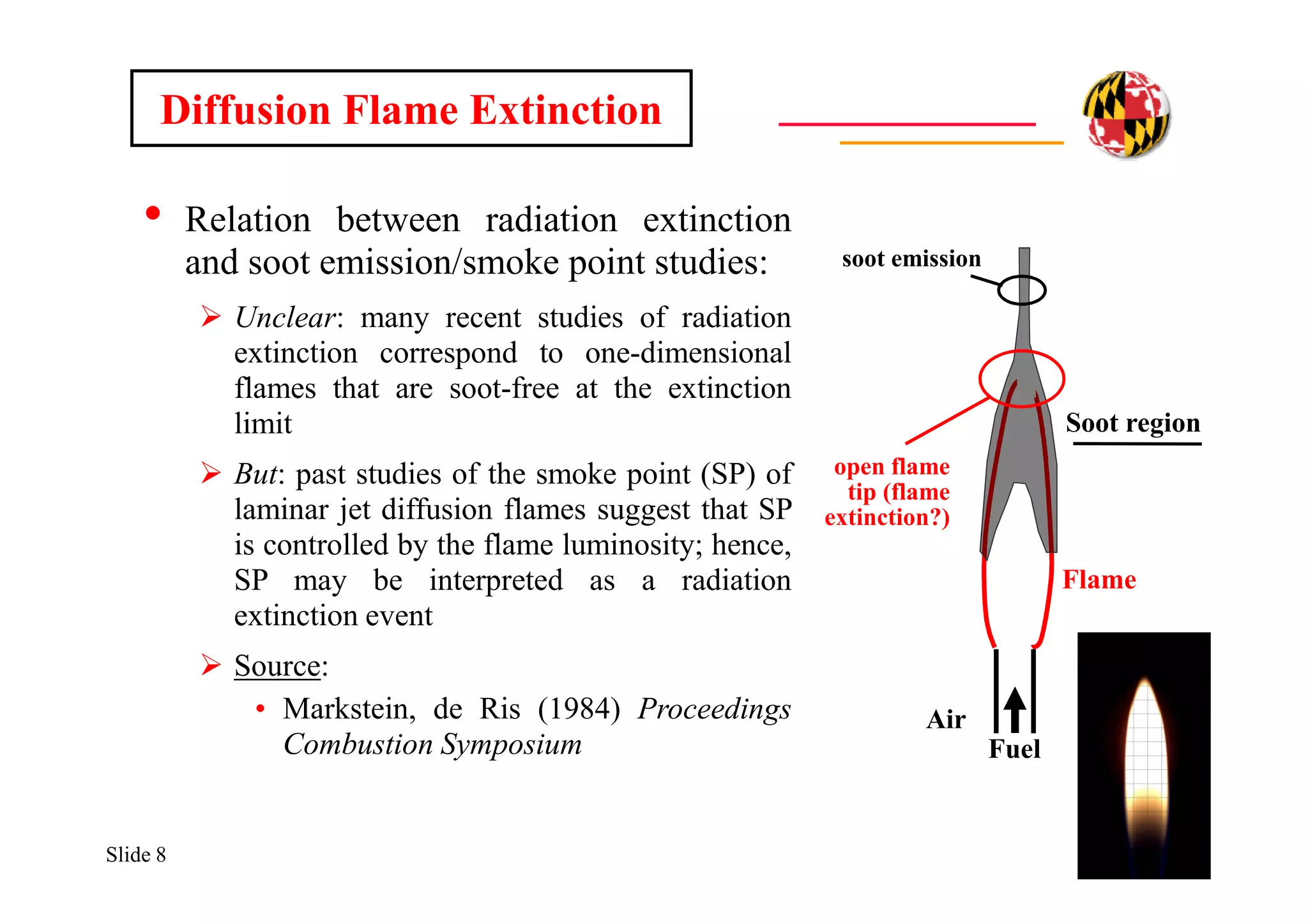
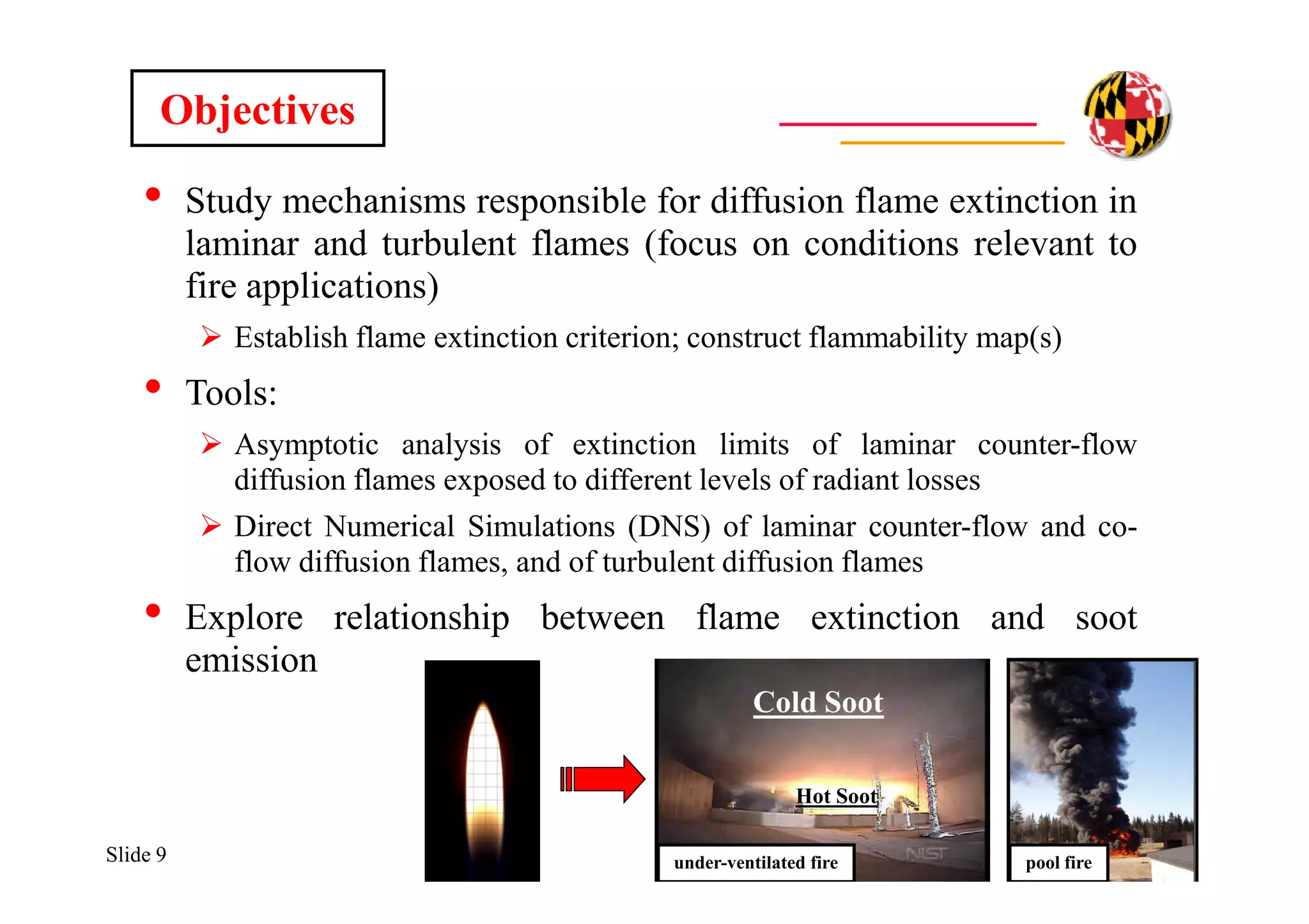
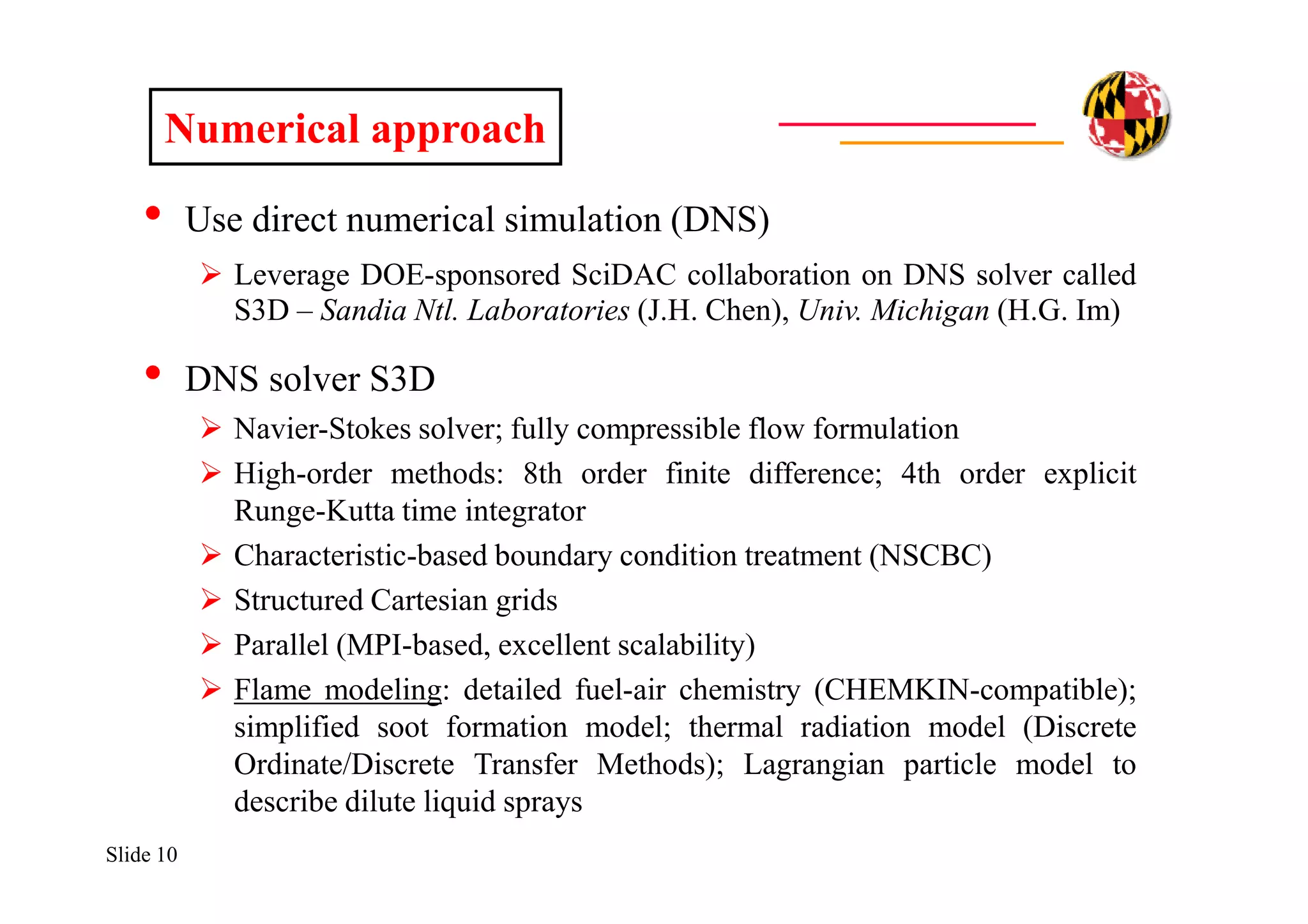
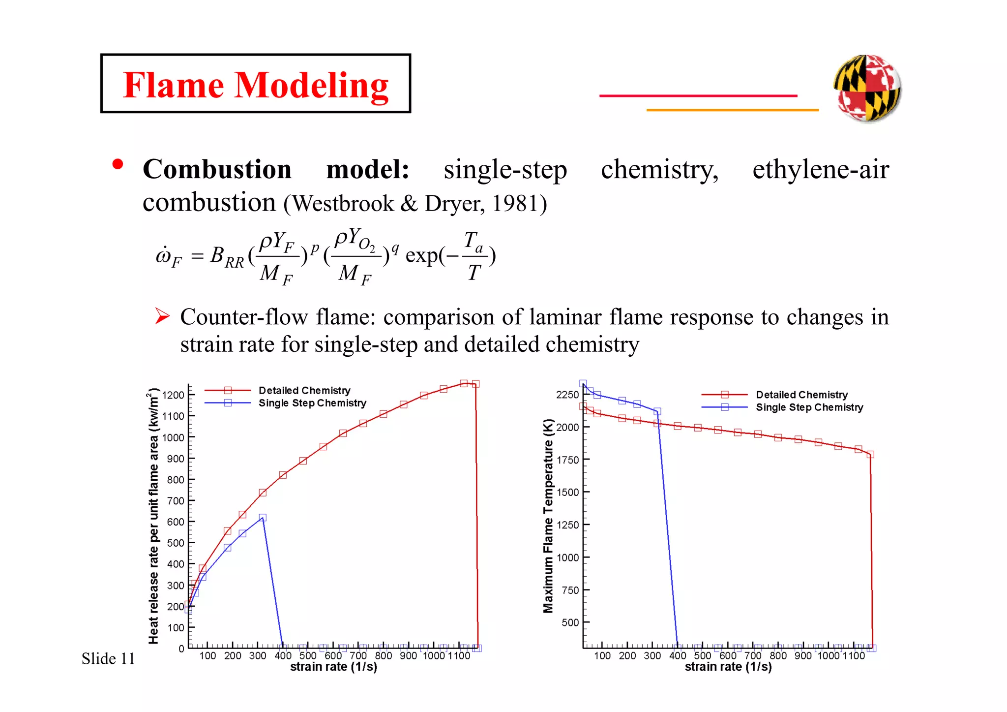
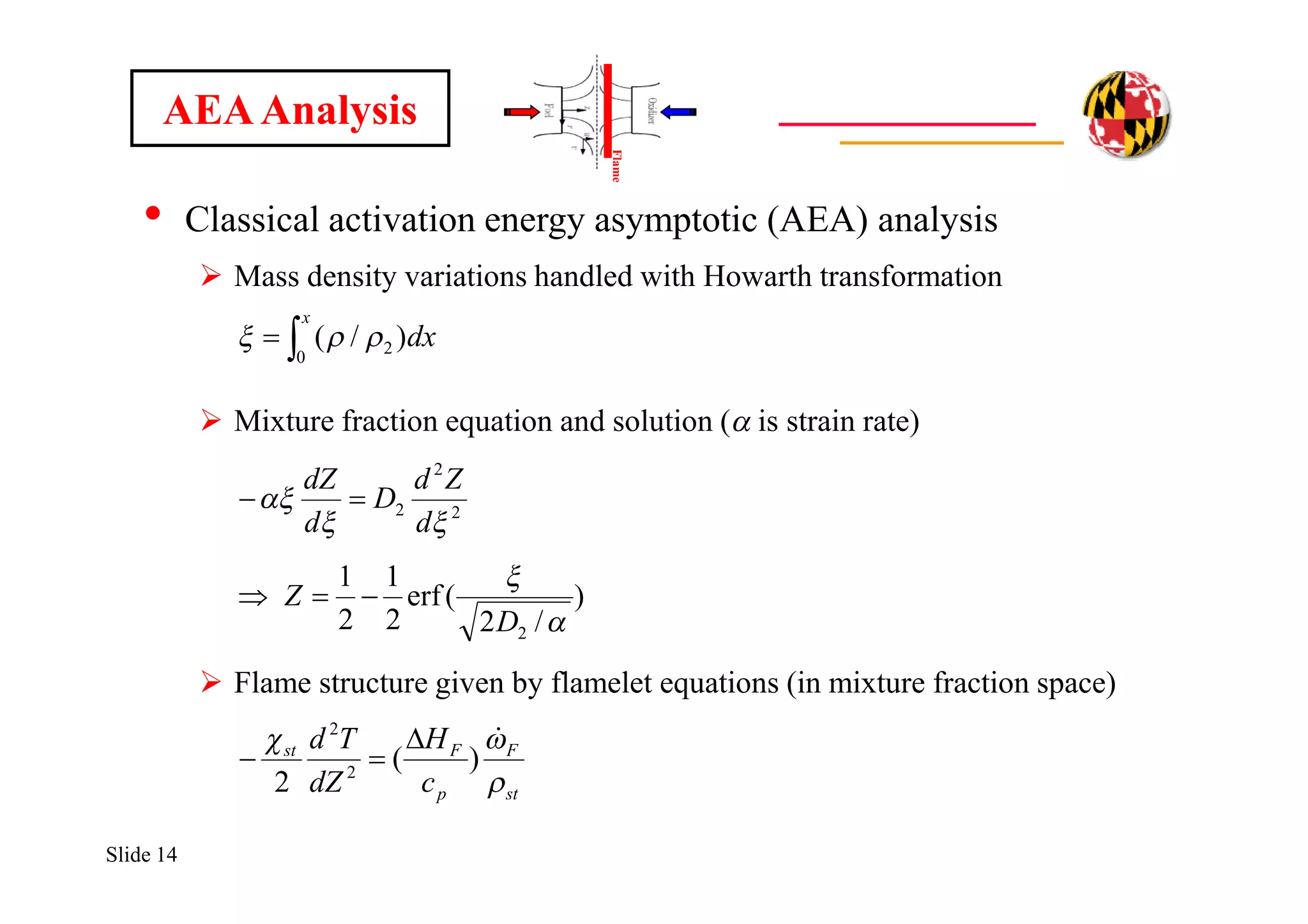
The document discusses using direct numerical simulation to study radiation-driven flame extinction in fires. It motivates the study by explaining how flame extinction impacts combustion systems and fire applications. It outlines the objectives to establish flame extinction criteria, construct flammability maps, and explore the relationship between extinction and soot emission. It describes the numerical approach using a DNS solver and models for chemistry, soot formation, and thermal radiation transport. Classical asymptotic analysis is also discussed for analyzing flame structure with and without radiation and soot. Laminar counter-flow flames will be used to obtain flame structure as a function of stretch from ultra-high to ultra-low values.
![Slide 13
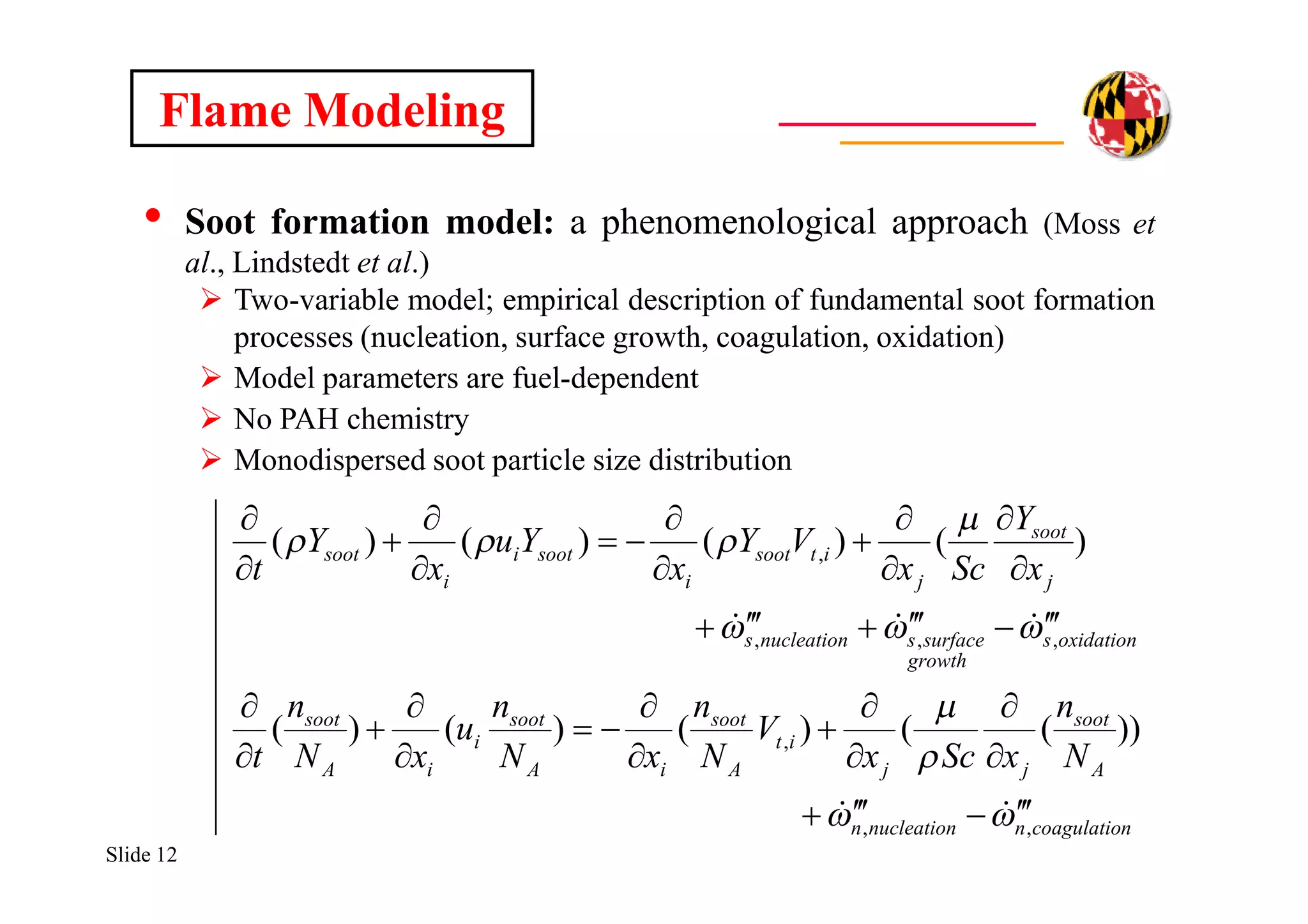
Flame Modeling
• Thermal radiation transport model: non-scattering, gray gas
assumption; Discrete Transfer Method (Lockwood & Shah, 1981)
Radiative transfer equation
Mean absorption coefficient [m-1]
• ap,i is the Planck mean absorption coefficient for species i [m-1 atm-1]
and is obtained from tabulated data (TNF Workshop web site)
• ksoot is the soot mean absorption coefficient [m-1]
AbsorptionEmission
4
)/( IT
ds
dI
sootCOCOOHOH axaxp )( 2222
-1-1
Km1817sootCTYCTfC sootsootsootvsootsoot )/( ](https://image.slidesharecdn.com/86fce12d-ad8e-4a58-a233-dac2bfcb6758-161023180038/75/RadiationDrivenExtinctionInFires-13-2048.jpg)
![Slide 15
• Classical decomposition into inner/outer layers
Perform asymptotic expansion in terms of small parameter e
Inner layer problem
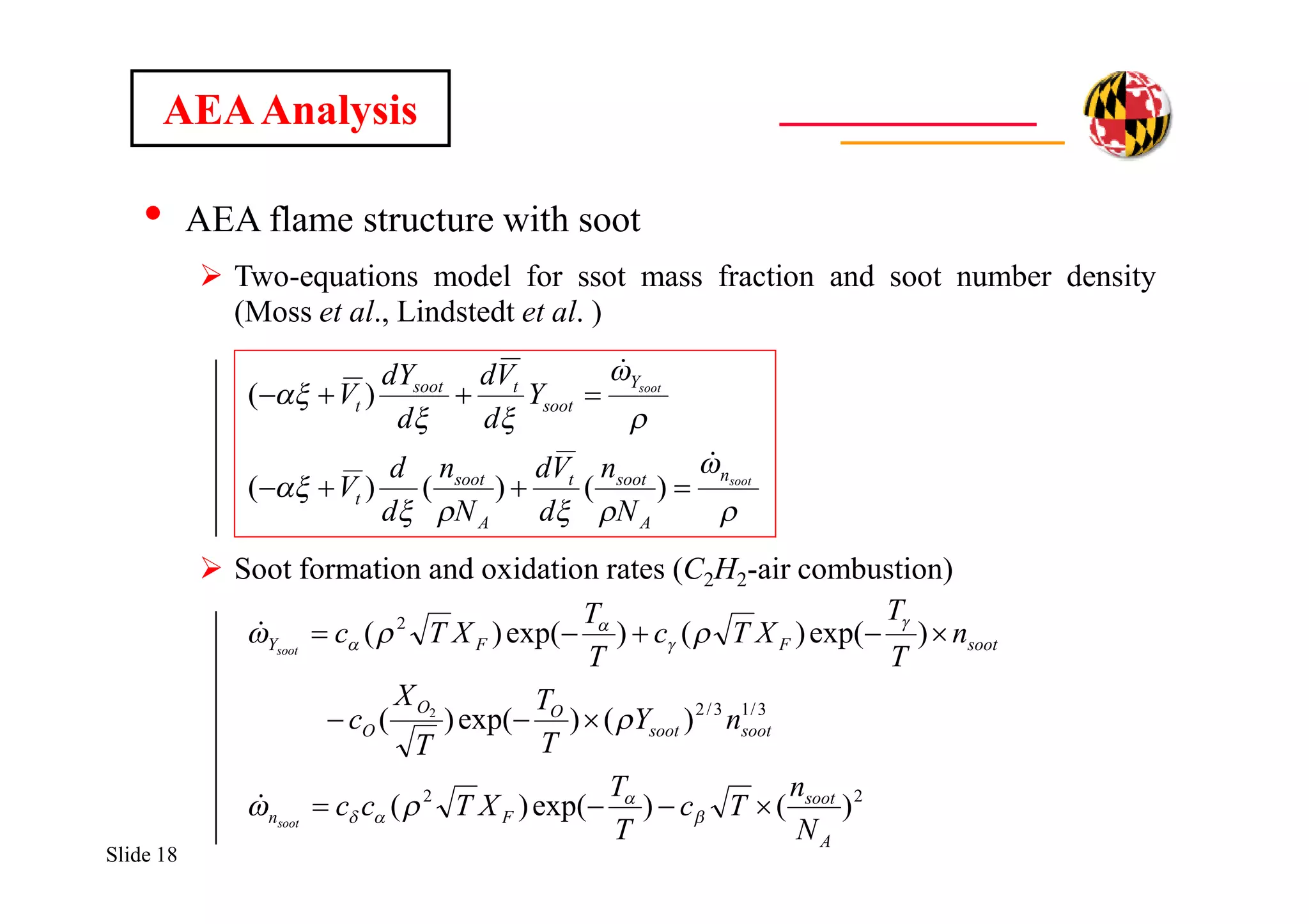
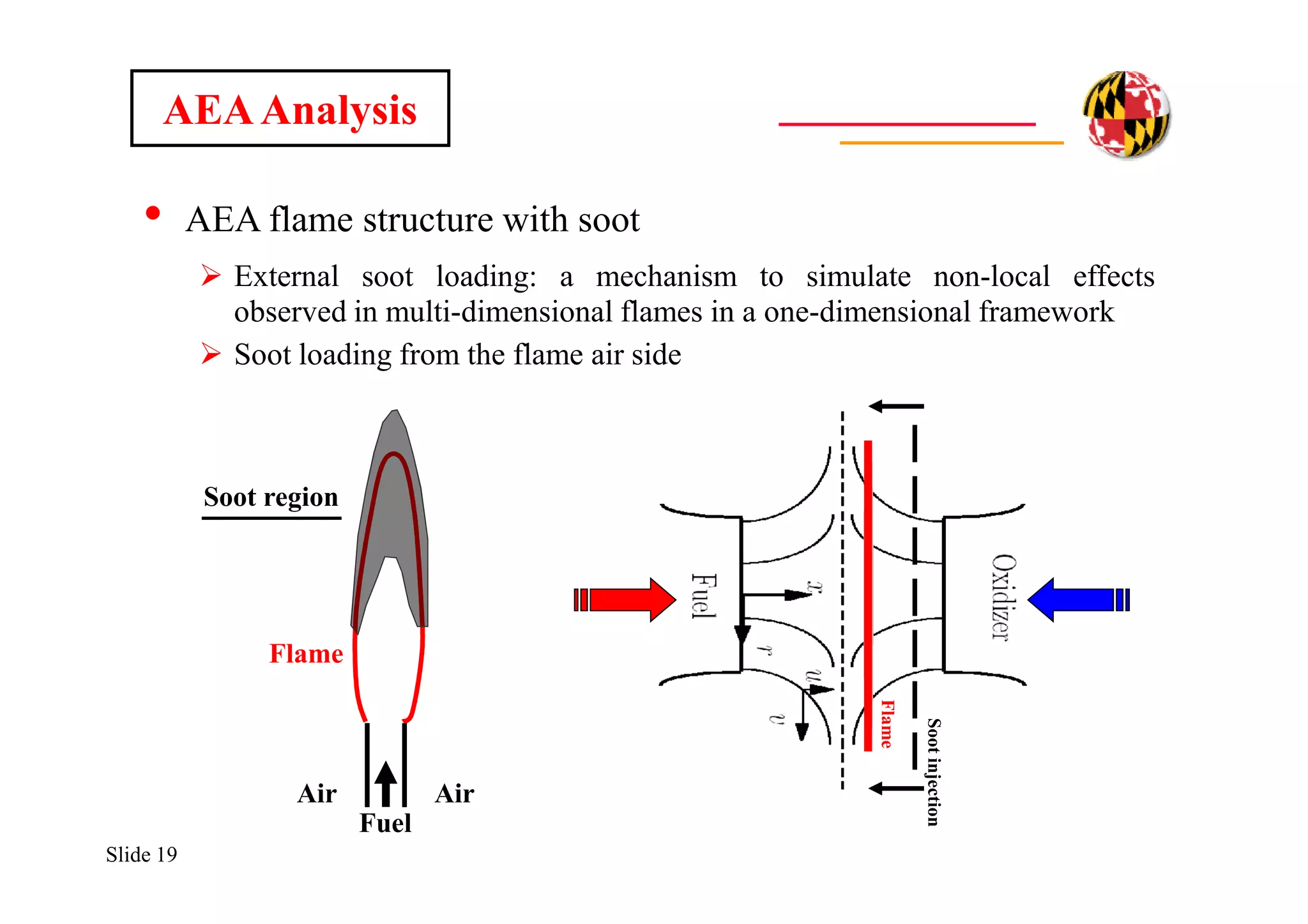
AEAAnalysis
)exp(]
)1(
[][
)(;)()(
2
2
221,
q
st
stp
st
p
FF
st
Z
Z
d
d
OZZO
c
YH
TT
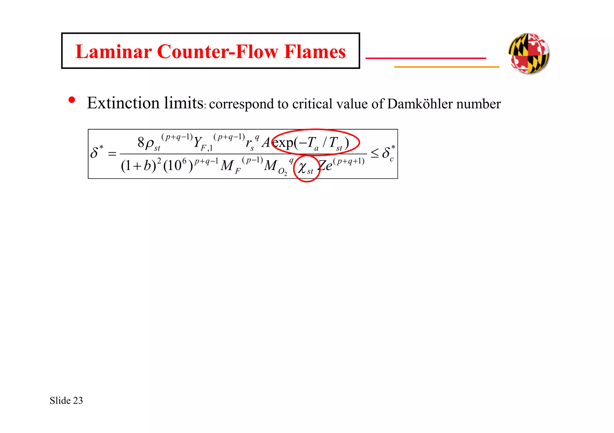
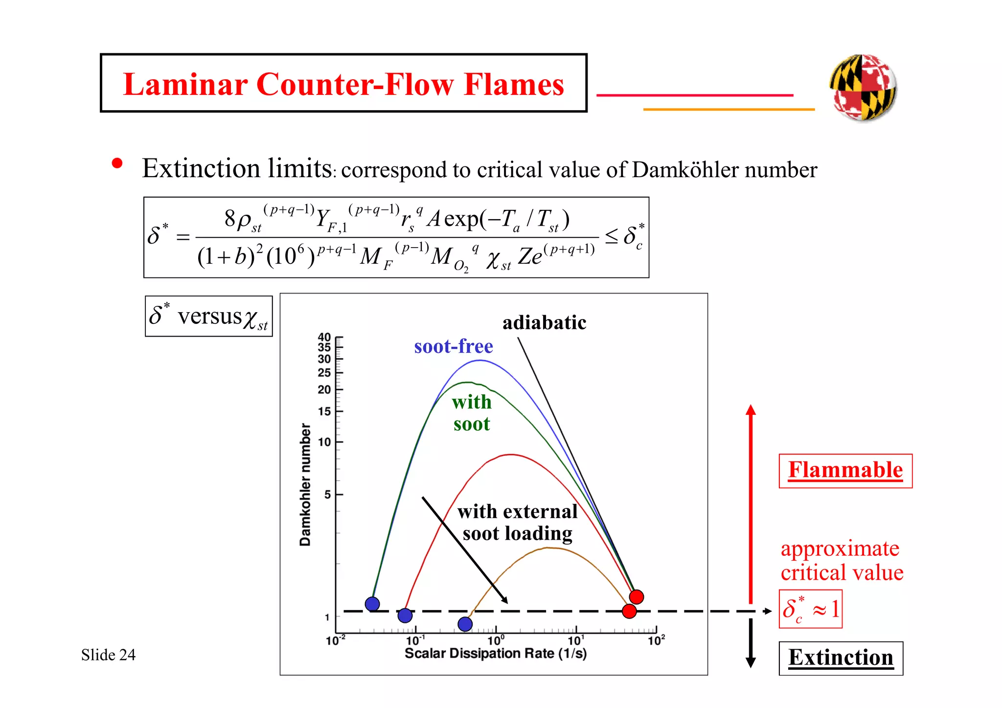
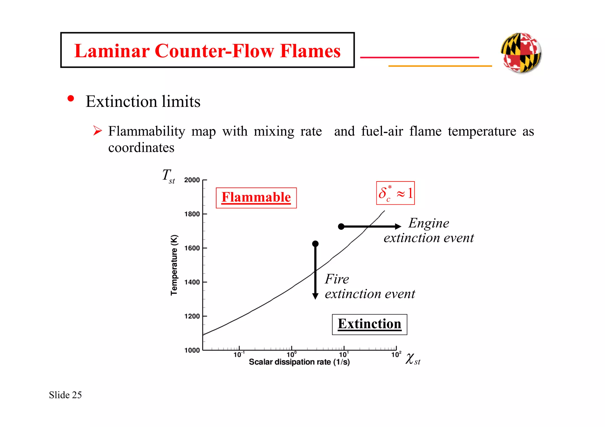
(d is a reduced Damkohler number)
)(
)(1
1,
2
FF
p
a
st
YH
c
T
T
Ze
)1/()/(;1)/( stst ZZdddd ](https://image.slidesharecdn.com/86fce12d-ad8e-4a58-a233-dac2bfcb6758-161023180038/75/RadiationDrivenExtinctionInFires-15-2048.jpg)
![Slide 17
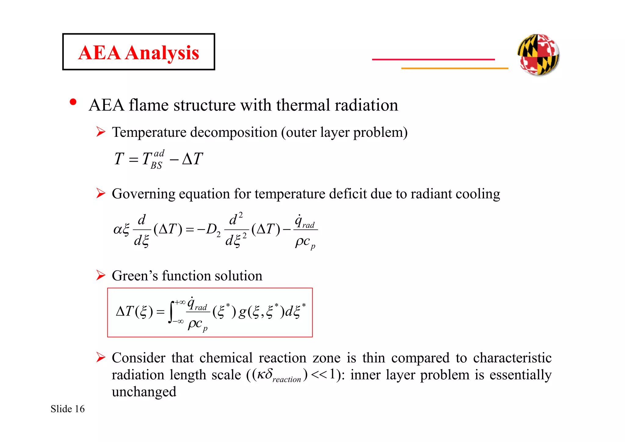
• AEA flame structure with thermal radiation
Green’s function solution
Emitting/absorbing medium (spectrally-averaged gray)
Planck mean aborption coefficient:
Analytical expression for G (as a function of optical depth t):
AEAAnalysis
)4( 4
GTqrad
***
),()()(
dg
c
q
T
p
rad
TfCaxaxp vsootOHOHCOCO )( 2222
]')'()'(')'()'(
)()([2
1
0
1
22,21,
R
dEIdEI
EIEIG
bb
Rbb
](https://image.slidesharecdn.com/86fce12d-ad8e-4a58-a233-dac2bfcb6758-161023180038/75/RadiationDrivenExtinctionInFires-17-2048.jpg)