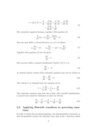
1. The document analyzes the effect of radiation on flame structure and extinction in a one-dimensional planar diffusion flame. A simplified configuration is adopted where quantities depend on the flame normal direction only. 2. The governing equations are transformed to a mass-weighted coordinate system using the Howarth transformation to simplify the treatment of density. Radiation is incorporated as a small perturbation using a dimensionless parameter defined as the product of the radiation absorption coefficient and a characteristic length scale. 3. Radiation lowers the flame temperature, affecting the reaction rate. The radiation absorption term in the energy equation is obtained from the radiation transport equation, appearing as a non-local integral that is treated using Green's functions.

1. Asymptotic analysis of radiative extinction in
a one-dimensional planar di↵usion flame
Praveen Narayanan
January 28, 2009
1 Introduction
In this study, the role of radiation is analysed to understand its e↵ect on
flame structure and extinction. A simplified, one dimensional configuration
is adopted, in which pertinent quantities are all one-dimensional, with the ex-
ception of the velocity field. The two dimensional Howarth transformation is
used to transform the governing equations into mass weighted coordinates in
order to simplify the treatment of density. The chemical reaction source term
is handled in conventional fashion as a singularity, resolved using matched
asymptotic expansions. The manifestation of radiation is in lowering the
flame temperature which then a↵ects the reaction rate significantly. The
form of the inner expansions is not a↵ected by radiation, and is described by
a purely reactive-di↵usive structure. However, the strength of the reaction
term is dictated by reduction in temperature brought about by radiation.
The treatment of the radiatively active outer layer is achieved by observing
that radiative length scale, as dictated by the inverse of the absorption co-
e cient is large compared to the di↵usion length scales. Thus radiation can
be incorporated as a small perturbation, the functional form of which may
be su ciently described by the leading order (or unperturbed) temperatures
in the respective emission and absorption terms. The outer region can then
be solved using a Green function as a convolution. The radiation terms may
also be treated equivalently using a regular perturbation expansion using the
small parameter identified above.
The radiation absorption term in the energy equation is obtained from the
radiation transport equation, with use being made of there being azimuthal
symmetry about the polar axis formed by the flame normal in spherical co-
ordinates. As mentioned above, absorption is accommodated in the current
1

2. framework from the leading order temperatures, and requires no special treat-
ment. However, being a non-local quantity, it appears as a non-local integral
over space. It is mentioned in passing (perhaps naively) that the utility of
Green’s functions is especially apparent in this case with non-singular (and
non-local) radiation terms. From the author’s cursory perusal of Mathemat-
ical Physics literature, the use of Green’s functions is a common procedure
(notable examples are in electromagnetism, quantum mechanics, and astro-
physics) to solve di↵erential equations with source terms.
2 Governing equations
2.1 Howarth transformation
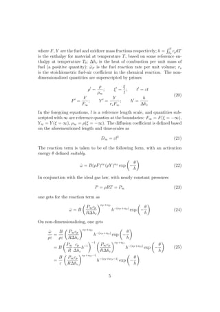
Density weighted coordinates are used, in conformity with Carrier, Fendell
and Marble [1] that greatly simplifies the analysis. The transformation is
described here in brief. For more extensive notes, Dr. Howard Baum’s [3]
document may be referred to.
Consider a two dimensional planar flame configuration in which the flame
normal is along the x direction; u and v being the velocities in the x and y
directions and ⇢ being the density. The equation of continuity is
@⇢
@t
+
@(⇢u)
@x
+
@(⇢v)
@y
= 0 (1)
A mass weighted coordinate is defined as
⇠ =
Z x
1
⇢
⇢1
dx (2)
where ⇢1 = ⇢(x = 1, y) = ⇢(x = 1) because of one-dimensionality in
this planar configuration. Transform the equations into this coordinate sys-
tem comprised of X = ⇠,Y = ⌘ and T = t with the following transformation
rules
x = x(⇠, Y, T) )
@
@x
=
@
@⇠
@⇠
@x
+
@
@Y
@Y
@x
+
@
@T
@T
@x
=
@
@⇠
@⇠
@x
=
⇢
⇢1
@
@⇠
(3)
y = y(⇠, Y, t) )
@
@y
=
@
@⇠
@⇠
@y
+
@
@Y
@Y
@y
+
@
@t
@y
@t
=
@
@⇠
@⇠
@y
+
@
@Y
(4)
2

3. t = t(⇠, Y, T) )
@
@t
=
@
@⇠
@⇠
@t
+
@
@Y
@Y
@t
+
@
@T
@T
@t
=
@
@⇠
@⇠
@t
+
@
@T
(5)
The continuity equation becomes, together with equation (2)
@
@x
(⇢u + ⇢1
@⇠
@t
) +
@(⇢v)
@y
= 0 (6)
Now one may define a stream function (x, y, t) as follows
⇢1
@
@x
= ⇢v; ⇢1
@
@x
= (⇢u + ⇢1
@⇠
@t
) (7)
Together with equation (2) the this gives
@
@⇠
= v (8)
One can now define a normal transformed velocity U(⇠, Y, t) as
@
@Y
= U (9)
A constant density version of the continuity equation may now be written as
@v
@Y
+
@U
@⌘
= 0 (10)
The velocity U is obtained from the equation (7) as
U =
1
⇢1
@⇠
@t
+
⇢
⇢1
u + v
@⇠
@y
(11)
The continuity equation may now into a form, after suitable manipulation,
to preseve the convective derivative so that one obtains
D
Dt
=
@
@T
+ U
@
@⇠
+ v
@
@Y
⌘
˜D
˜DT
(12)
2.2 Applying Howarth transform to governing equa-
tions
In order to obtain the governing equations, one-dimensionality is assumed, so
that all quantities (except the velocities) vary only in the x direction, which
3

4. is normal to the flame. The velocity in the direction normal to the flame in
this new coordinate system is obtained from the equation (10) as
U =
Z ⇠
0
@v
@Y
d⇠ (13)
If a constant strain @v/@Y = ", together with a reference velocity of zero at
⇠ = 0 is assumed (which are perfectly reasonable assumptions), one gets
U =
Z ⇠
0
@v
@Y
d⇠ = "⇠ (14)
In the undermentioned, T and Y are replaced later by t and y to retain
the usual notation. The transport operator is now transformed into mass
weighted coordinates.As mentioned in the foregoing, quantities of interest
are only assumed to depend on x and t. Furthermore, unity Lewis numbers
are assumed so that the di↵usion coe cient may be denoted by a quantity
D. The untransformed transport operator is
⇢L ⌘ ⇢
@
@t
+ ⇢u
@
@x
@
@x
✓
D⇢
@
@x
◆
@
@y
✓
D⇢
@
@y
◆
(15)
Upon introducing the transformation, and ignoring Y dependence, one gets
⇢
@
@t
+ ⇢u
@
@x
= ⇢
✓
@
@T
"⇠
@
@⇠
◆
(16)
The di↵usion terms are manipulated, using the transformation (2) as follows
@
@x
✓
⇢D
@
@x
◆
=
⇢
⇢1
@
@⇠
✓
D⇢
⇢
⇢1
@
@⇠
◆
=
⇢
⇢2
1
@
@⇠
✓
D⇢2 @
@⇠
◆ (17)
Now, if one makes the simplification that D⇢2
is nearly constant in flows of
interest, one may pull out this quantity as D⇢2
= D1⇢2
1. One may replace
T with t to obtain
L ⌘
@
@t
"⇠
@
@⇠
D1
@2
@⇠2
(18)
2.3 Non-dimensionalization
The governing equations for species mass and energy are
L(F) = ⇢ 1
˙!F
⇢L(Y ) = ⇢ 1
rs ˙!F
⇢L(h) = ⇢ 1
hc ˙!F + ⇢ 1
5 ·~qR
(19)
4

5. where F, Y are the fuel and oxidizer mass fractions respectively; h =
R T
T0
cpdT
is the enthalpy for material at temperature T, based on some reference en-
thalpy at temperature T0; hc is the heat of combustion per unit mass of
fuel (a positive quantity); ˙!F is the fuel reaction rate per unit volume; rs
is the stoichiometric fuel-air coe cient in the chemical reaction. The non-
dimensionalized quantities are superscripted by primes
⇢0
=
⇢
⇢1
; ⇠0
=
⇠
l
; t0
= "t
F0
=
F
F1
; Y 0
=
Y
rsF1
; h0
=
h
hc
(20)
In the foregoing equations, l is a reference length scale, and quantities sub-
scripted with 1 are reference quanties at the boundaries: F1 = F(⇠ = 1),
Y1 = Y (⇠ = 1), ⇢1 = ⇢(⇠ = 1). The di↵usion coe cient is defined based
on the aforementioned length and time-scales as
D1 = "l2
(21)
The reaction term is taken to be of the following form, with an activation
energy ✓ defined suitably.
˙! = B(⇢F)⌫F
(⇢Y )⌫O
exp
✓
✓
h
◆
(22)
In conjunction with the ideal gas law, with nearly constant pressures
P = ⇢RT = P1 (23)
one gets for the reaction term as
˙! = B
✓
P1cp
R hc
◆⌫F +⌫O
h (⌫F +⌫O)
exp
✓
✓
h
◆
(24)
On non-dimensionalizing, one gets
˙!
⇢"
=
B
⇢"
✓
P1cp
R hc
◆⌫F +⌫O
h (⌫F +⌫O)
exp
✓
✓
h
◆
= B
✓
P1
R
cp
hc
h 1
◆ 1 ✓
P1cp
R hc
◆⌫F +⌫O
h (⌫F +⌫O)
exp
✓
✓
h
◆
=
B
"
✓
P1cp
R hc
◆⌫F +⌫O 1
h (⌫F +⌫O 1)
exp
✓
✓
h
◆
(25)
5

6. From the above, one may identify the multiplying quantities on the right hand
side as the first Damk¨ohler number D1 (notation consistent with Carrier,
Fendell and Marble).
D1 =
B
"
✓
P1cp
R hc
◆⌫F +⌫O 1
(26)
The small parameters for the reaction zone may either be taken as the inverse
of the first Damk¨ohler number D1 for large Damk¨ohler number expansions
or as h2
⇤/✓ where h⇤ is the flame temperature in a large activation energy
expansion. The treatment is postponed until later. In either case, it will
be seen that the form of the inner expansion is not a↵ected by the presence
of radiation. The radiation terms are non-dimensionalized with a reference
absorption coe cient ¯ and a reference radiation intensity ¯I. This, in fact,
furnishes a small parameter for the radiation source term.
5 · ~qR ⇠ ¯¯Ib
⇤
⇠ ¯ T4
⇤ (27)
where the subscript ⇤ denotes quantities at the flame, located at ⇠⇤; Ib(⇠) =
⇡ T(⇠)4
is the black body radiation intensity. The emission term is inspected
to provide a suitable small quantity for radiation.
5 · qR ⇠ ¯ T4
⇤
Or
5 · qR
⇢ hc"
⇠
¯ T4
⇤
⇢⇤ hc"
= ¯l
T4
⇤
⇢⇤ hcl"
(28)
Plugging in typical values taken as T⇤ = 2000 K, ⇢⇤ = 0.2 kg/m3
, hc =
32 MJ/kg, one gets
5 · qR
⇢ hc"
⇠
¯l
l"
(5.67 ⇥ 10 8)(2000)4
0.2 ⇥ (32 ⇥ 106)
=
✓
0.14
"l
◆
l
(29)
In the current problem, l is a small number because the radiation length
scale (⇠ 1/) is expected to be much larger than the di↵usion length scale
(⇠ l). Thus one can now define a small parameter ✏ such that
✏ = l ⌧ 1 (30)
Furthermore, the quantity multiplying l in the equation (29) is assumed to
be O(1). This is a reasonable assumption for small flames, and large strain
rates. The intent is to demonstrate that the product
✓
0.14
"l
◆
¯l ⌧ 1 (31)
6

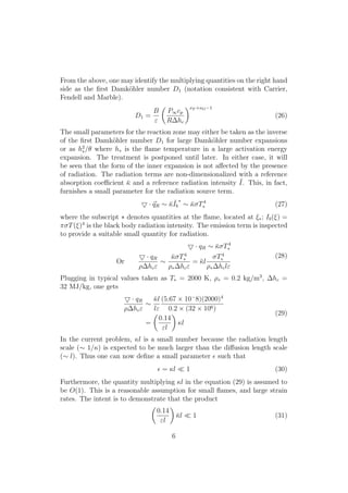
7. and not per se, that 0.14/("l) ⇠ O(1) in that one wants to be able to show
that the non-dimensionalized radiation source term is much smaller than
unity so that the unperturbed (or radiation free) temperatures may be used
as a first approximation for these terms. Radiation is then a known field and
may be used in calculating the flame temperature.
To get back to the main discussion it therefore transpires that in the
non-dimensional equations the radiation term is multiplied by a quantity of
O(✏). This will be used in the analysis later. In order to make the notation
consistent, the radiation term is now scaled in terms of enthalpy instead of
temperature. If one were to non-dimensionalize 
0
=

¯
(32)
and drop the prime symbol in the equations, one gets for the emission term
qR,E
5 · qR,E
⇢" hc
= ¯l
✓
T4
hc"⇢
◆
= (¯l)
✓
hc"l
h4
c
c4
p
h4
⇢
◆
= (¯l)
✓
hc"l
◆ ✓
h4
ch4
c4
p
◆ ✓
RT
P1
◆

= (¯l)
✓
hc"l
◆ ✓
h4
ch4
c4
p
◆ ✓
RcpT
hc
hc
cpP1
◆

= (¯l)
✓
hc"l
◆ ✓
h4
ch4
c4
p
◆ ✓
h
hcR
cpP1
◆

= (¯l)
"✓
hc"l
◆ ✓
hc
cp
◆5 ✓
R
P1
◆
h5
#
⇠ O(¯l)
(33)
The absorption term is obtained in the document [2].
One may then write the radiation terms (which will now include both
emission and absorption) as
5 · ~qR
⇢" hc
= (¯l)f(h(⇠), (⇠)) = (¯l)g(⇠) ⇠ O(¯l) (34)
The energy equation becomes
L(h) = D1h (⌫F +⌫O 1)
F⌫F
Y ⌫O
exp
✓
✓
h
◆
+ (¯l)g(⇠) (35)
7

8. The equations for fuel and oxidizer mass fractions are obtained from Scwhab-
Zeldovich relationships.
L(h + F) = (¯l)g(⇠) (36)
L(h + Y ) = (¯l)g(⇠) (37)
3 Inner expansions
The inner expansions may be carried out either with a large Activation En-
ergy expansion, or a large Damk¨ohler number expansion. For purposes of
illustration, a large Damk¨ohler number expansion is chosen. The large acti-
vation energy expansion is explored later, and is handled analogously to that
of numerous previous investigations. Consider the steady energy equation
⇠
dh
d⇠
d2
h
d⇠2
= D1h (⌫F +⌫O 1)
F⌫F
Y⌫O
exp
✓
✓
h
◆
+ (¯l)g(⇠) (38)
As in Carrier, Fendell and Marble, one takes the the inverse of the first
Damk¨ohler number = D 1
1 as the small parameter. Propose a stretched
inner coordinate for the boundary layer as
⌘ =
⇠ ⇠⇤
b
(39)
where ⇠⇤ is the flame location and b is a number to be determined shortly.
One writes
F(⇠) = F(⌘)
Y (⇠) = Y (⌘)
h(⇠) = H (⌘)
(40)
All pertinent quantities are now expanded as a power series of b
to first
order. Note that fuel and oxidizer are vanishing in the inner layer to leading
order.
F = 0 + b
F1
Y = 0 + b
Y1
H = H⇤
b
H1
(41)
Upon inserting the expansion (41) into equation (38) and rearranging (with
higher order terms included only where deemed useful for illustration), one
8

9. gets
⇠⇤
b
d
d⌘
(H⇤
b
H1)
1
2b
d2
d⌘2
(H⇤
b
H1)
= 1 b(⌫F +⌫O)
h (⌫F +⌫O 1)
⇤ F⌫F
1 Y ⌫O
1 exp
✓
✓
h⇤
◆
+ (¯l)g(⇠⇤)
(42)
It emerges from the above on multiplying throughout by b
and rearranging,
that the radiation term will be O( b
(¯l) and is negligible compared to the
reaction term, which is O(1). Also, the convective term may be neglected
compared to the di↵usion term. It transpires that the inner equation does
not feature the radiation term to leading order. Matching O(1) terms gives
b =
1
⌫F + ⌫O + 1
(43)
and the inner equation becomes
d2
H1
d⌘2
= h (⌫F +⌫O 1)
⇤ exp
✓
✓
h⇤
◆
F⌫F
1 Y ⌫O
1 (44)
One may notice that although the form of the inner equation is unaltered,
compared to the radiation free case, the strength of the reaction is reduced
because of a drop in temperature in the term
h (⌫F +⌫O 1)
⇤ exp
✓
✓
h⇤
◆
(45)
Notably, a small decrease in the temperature will lead to a large drop in the
chemical reaction rate because of exponential behavior of the function. The
exercise therefore boils down to determining the flame temperature given by
h⇤ with radiation. This is obtained from the outer solutions. The flame
location ⇤ is also obtained from the outer solutions. To leading order, this is
unaltered from the case with no radiation.
4 Outer solutions
The outer solutions may be postulated as a perturbation from the solution
obtained without radiation. To that end, it the species mass concentrations
are una↵ected, but the presence of the radiation source term will see an al-
teration in the flame temperature. One may propose the following expansion
for the enthalpy
h(⇠) = h0
(⇠; a
) + (¯l)h1
(46)
9

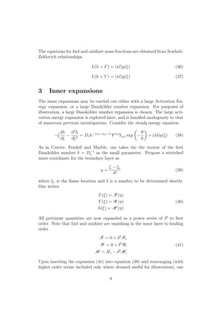
10. where h0
(⇠; a
) is the solution obtained without radiation (and is a known
function), and a is a quantity that is to be determined accordingly for the
fuel and oxidizer sides of the flame (also known). It can be seen that insofar
as radiation is concerned, one only needs the leading order behavior of h in
the expansion proposed above. This may be inserted in the outer equations
to obtain the flame temperature in the outer region. The equations may then
be solved using a regular perturbation expansion with ¯l as the expansion
parameter, or, more elegantly, by the use of Green’s functions.
4.1 Flame location
The flame location is the same as without radiation, because one can match
leading order solutions from the local Schwab-Zeldovich expansions. The
procedure is identical to that described in Carrier, Fendell and Marble. For
the local Schwab-Zeldovich relations one uses
L(F0
+ h0
) = 0
L(Y 0
+ h0
) = 0
(47)
This gives an expression for the flame location as
erf
✓
⇠⇤
p
2
◆
=
F1 Y1
F1 + Y1
(48)
4.2 Obtaining the flame temperature
4.2.1 Regular Perturbation
The flame temperature, as mentioned in the foregoing, may be determined
from a regular perturbation expansion for the temperature as follows
h(⇠) = h0
(⇠; a
) + (¯l)h1
(⇠) (49)
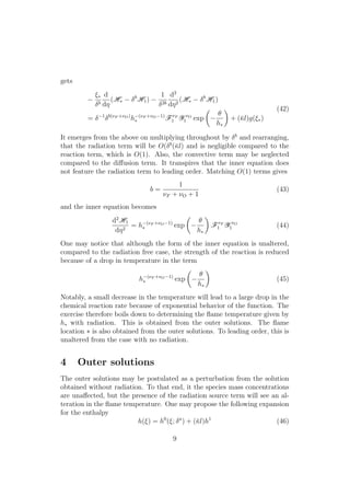
In the foregoing, h1
is a function that is smooth upto its first derivative so
that
[h1
]⇠⇤ = [h1
]⇠⇤+
✓
dh
d⇠
◆
⇠⇤
=
✓
dh
d⇠
◆
⇠⇤+
(50)
The function g(⇠) is entirely known because it only contains leading order
terms. One can then obtain for the O(¯kl) terms
L(h1
) = g0 (51)
10

11. with boundary conditions
h1
⇠= 1 = 0
✓
dh1
d⇠
◆
⇠= 1
= 0
h1
⇠=1 = 0
✓
dh1
d⇠
◆
⇠=1
= 0
(52)
In the aforementioned equation, it is expected that the conditions on the
derivatives should hold trivially.
4.2.2 Green’s function
As an alternative to regular perturbation, one may also use a Green’s function
approach to solve for the relevant quantities in the outer layers. One of the
advantages with this formalism is that it is easy to set up, and involves
much less labor than a regular perturbation. It is noted that the approach
works because the governing equations are linear. The procedure is briefly
illustrated below. For a more elaborate discussion Carrier and Pearson [4] or
any other text on ordinary di↵erential equations may be referred to. Consider
a linear di↵erential equation with the operator L
L =
d
d⇠
✓
p(⇠)
d
d⇠
◆
+ q(⇠) (53)
acting on the variable y to give the inhomogeneous problem
L y = f(⇠) (54)
If one were to find a Green’s function G(⇠, s), which is continuous in ⇠ and
di↵erentiable at all points except ⇠ = s, satisfying the boundary conditions
of the inhomogeneous problem (54) so that
L G = (⇠ s) (55)
where (⇠ s) is the Dirac Delta function, then upon multiplying both sides
by f(⇠) (a known function) and integrating with respect to s one gets
Z 1
1
L Gf(⇠)ds =
Z 1
1
f(⇠) (s ⇠)ds
= f(⇠)
(56)
11

12. Since the operator L is linear one can take it out of the integral to obtain
L
Z 1
1
G(⇠, s)f(⇠)ds = f(⇠) (57)
Inspection of equation (57) reveals that the integral in the LHS is the sought
solution.
y =
Z 1
1
G(⇠, s)f(⇠)ds (58)
One only needs to find a Green’s function, which can be done without much
di culty, as is shown in the forthcoming.
4.2.3 Application of Green’s function to find outer solutions
In this problem, the function f in the foregoing is replaced by the known
function g(⇠). Thus, one can determine the outer solution from the convolu-
tion
h =
Z 1
1
G(⇠, s)(¯l)g(⇠)ds (59)
Since this has known boundary conditions, the problem can be solved. One
may therefore obtain h⇤ for use in the inner equations (which has the same
boundary conditions as the case without radiation) and solve for the inner
temperature H. Extinction analysis can then be carried out by increasing the
radiation losses, which translates to a parametric variation of the coe cient
l.
4.2.4 Obtaining Green’s function for given problem
The Green’s function for this problem is obtained by solving the equivalent
homogeneous problem, defined as
L(G(⇠, s)) = (⇠ s) (60)
satisfying the boundary conditions
G( 1, s) = h 1
G(1, s) = h1
(61)
It may be added, superfluously, that the Green’s function is constructed so
as to satisfy the boundary conditions of the original inhomogeneous prob-
lem. One is referred to the text by Carrier and Pearson [4] for details. The
12

13. Green’s function constructed above is continuous over the domain, but has
a discontinuous derivative at ⇠ = s. Rewrite the di↵erential equation as
d
d⇠
✓
p(⇠)
dG
d⇠
◆
= 0 (62)
where
p(⇠) = exp
✓
⇠2
2
◆
(63)
Integrate (62) to get
G(⇠, s) = h 1 + A(s)
Z ⇠
1
exp
✓
µ2
2
◆
dµ 1 < ⇠ < s
= h1 + B(s)
Z 1
⇠
exp
✓
µ2
2
◆
dµ s < ⇠ < 1
(64)
Call the linearly independent solutions obtained above, on either side of ⇠ = s
as 1 and 2.
A(s) 1(⇠) = G(⇠, s) h 1; 1 < ⇠ < s
B(s) 2(⇠) = G(⇠, s) h1; s < ⇠ < 1
(65)
The constants A(s) and B(s) (invariant with respect to ⇠) may be deter-
mined by imposing continuity of the Green’s function, and discontinuity of
its derivative at ⇠ = s. Imposing continuity of G at ⇠ = s one gets
h 1 + A(s) 1(s) = h1 + B(s) 2(s) (66)
The jump condition for the derivative at ⇠ = s is given by
G⇠(s+, s) G⇠(s , s) =
1
p(s)
= exp
✓
s2
2
◆
(67)
where the subscript ⇠ refers to di↵erentiation with respect to ⇠. Equations
(66) and (67) may be solved to give A(s) and B(s) as follows
A(s) =
h 1 h1 + 2(s+)
p
2⇡
B(s) =
h 1 h1 1(s )
p
2⇡
(68)
The outer solution to the energy equation may now be written in terms of
the Green’s function
h(⇠) =
Z 1
1
G(⇠, s)f(⇠)ds
=
Z ⇠
1
[h1 + B(s) 2(⇠)]f(⇠)ds +
Z 1
⇠
[h 1 + A(s) 1(⇠)]f(⇠)ds
(69)
13

14. 5 Conclusions
A tentative framework has been laid out for the asymptotic analysis of the
radiating flame. The problem extends upon the work by Carrier, Fendell
and Marble by adding radiation as a small perturbation. The resulting small
decrease in flame temperature is expected to lead to a more drastic decrease
in reaction rate, and eventually cause flame extinction. The formulation is
general insofar as to account for both emission and absorption. As further
work, the details will be worked out for the regular perturbations and the
Green’s functions, so as to subsequently perform an analysis of extinction.
Large activation energy asymptotic expansions will also be explored to
obtain an extinction criterion. Since only the inner equations are relevant for
the extinction analysis, one may see that it is readily amenable to the form
proposed by Li˜nan from which can be extracted a criterion as reported in
other investigations. However, it is critical to obtain the flame temperature
from the outer expansions in this case as well.
References
[1] Carrier, G., F., Fendell, F., E., Marble, F., E., “The e↵ect of
strain rate on di↵usion flames”, SIAM Journal of Applied Math-
ematics, 28, No. 2, March 1975.
[2] Narayanan, P., “Expression for radiant energy absorption for use
in energy equation”, Internal document.
[3] Baum, H. R., “Notes on the Howarth Transformation”, “Internal
document.
[4] Carrier, G. F., Pearson, C. E. “Ordinary Di↵erential Equations,
Theory and Practice”, SIAM Classics in Applied Mathematics,
1992.
14