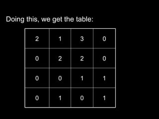
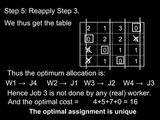
The Hungarian method is an algorithm that solves assignment problems in polynomial time. It was developed by Harold Kuhn in 1955. The method finds the optimal assignment between two equally sized sets that maximizes the total value of assignments. It works by constructing and updating a cost matrix through row and column reductions until the optimal assignment is revealed.

1. Assignment Problems
Compiled By: Group c
Sandeep Amin

2. The Hungarian method is a
combinatorial optimization algorithm which
solves the assignment problem in
polynomial time and which anticipated later
primal-dual methods. It was developed and
published by Harold Kuhn in 1955, who gave
the name "Hungarian method" because the
algorithm was largely based on the earlier
works of two Hungarian mathematicians:
Dénes Kőnig and Jenő Egerváry.

3. Suppose there are two machines in the press and two
operators are engaged at different rates to operate
them. Which operator should operate which machine for
maximizing profit?
Similarly, if there are n machines available and n
persons are engaged at different rates to operate them.
Which operator should be assigned to which machine to
ensure maximum efficiency?
While answering the above questions we have to think
about the interest of the press, so we have to find such
an assignment by which the press gets maximum profit
on minimum investment.
Such problems are known as "assignment problems"

4. Phase 1: Row and column
reductions
Step 0: Consider the given cost matrix
Step 1: Subtract the minimum value of each
row from the entries of that row, to obtain
the next matrix.
Step 2: Subtract the minimum value of each
column from the entries of that column , to
obtain the next matrix.
Treat the resulting matrix as the input for
phase 2.

6. The Hungarian Method
Consider the assignment problem:
Row
Job
Min
1 2 3 4
1 8 6 5 7 p1 = 5
2 6 5 3 4 p2 = 3
Worker
3 7 8 4 6 p3 = 4
4 6 7 5 6 p4 = 5

7. Step 1: From each entry of a row, we subtract
the minimum value in that row and get the
following reduced cost matrix:
3 1 0 2
3 2 0 1
3 4 0 2
1 2 0 1
Column q1=1 q2=1 q3=0 q4=1
Minimum

8. Step 2: From each entry of a column, we
subtract the minimum value in that column
and get the following reduced cost matrix:
2 0 0 1
2 1 0 0
2 3 0 1
0 1 0 0

9. Step 3: Now we test whether an assignment
can be made as follows. If such an assignment
is possible, it is the optimal assignment.
•Examine the first row. If there is only one zero
in that row, then make an ( ) and cross ( )
all the other zeros in the column passing
through the surrounded zero and draw a
vertical line on that column
•Then starting with the first column if there is
one zero then make an ( ) cross all the zero
in that row & draw horizontal line on that row
cont till all zero are crossed or even assignment

10. Step 3(a) gives the following table.
2 0 0 1
2 1 0 0
2 3 0 1
0 1 0 0
Step 3(b): Now repeat the above procedure for
columns. (Remember to interchange row and
column in that step.)

11. Step 3(b) gives the following table.
2 0 0 1
2 1 0 0
2 3 0 1
0 1 0 0

12. If there is now a surrounded zero in each row
and each column, the optimal assignment is
obtained.
In our example, there is a surrounded zero in
each row and each column and so the optimal
assignment is: Hrs
Worker 1 is assigned to Job 2 = 6
Worker 2 is assigned to Job 4 = 4
Worker 3 is assigned to Job 3 = 4
Worker 4 is assigned to Job 1 = 6
Minimum total time = 20 hrs
The optimal solution is unique

13. If the final stage is reached (that is all the
zeros are either surrounded or crossed) and
if there is no surrounded zero in each row
and column, it is not possible to get the
optimal solution at this stage. We have to do
some more work. Again we illustrate with a
numerical example.
Solve the following unbalanced assignment
problem (Only one job to one man and only
one man to one job): 7 5 8 4
5 6 7 4
8 7 9 8

14. Since the problem is unbalanced, we add a
dummy worker 4 with cost 0 and get the
following starting cost matrix:
Job Row Min
7 5 8 4 p1=4
Worker 5 6 7 4 p2=4
8 7 9 8 p3=7
0 0 0 0 p4=0 Dummy
Applying Step 1, we get the reduced cost
matrix

15. 3 1 4 0
1 2 3 0
1 0 2 1
0 0 0 0
Now Step 2 is Not needed. We now apply
Step 3(a) and get the following table.

16. 3 1 4 0
1 2 3 0
1 0 2 1
0 0 0 0
Now all the zeros are either surrounded or
crossed but there is no surrounded zero in
Row 2. Hence assignment is NOT possible.
We go to Step 4.

17. Step 4(b) Select the smallest element, say, u, from
among all elements uncovered by all the lines.
In our example, u = 1
Step 4(c) Now subtract this u from all uncovered
elements but add this to all elements that lie at the
intersection of two lines
3 1 4 0
1 2 3 0
1 0 2 1
0 0 0 0

18. Doing this, we get the table:
2 1 3 0
0 2 2 0
0 0 1 1
0 1 0 1

19. Step 5: Reapply Step 3.
We thus get the table
2 1 3 0
0 2 2 0
0 0 1 1
0 1 0 1
Thus the optimum allocation is:
W1 → J4 W2 → J1 W3 → J2 W4 → J3
Hence Job 3 is not done by any (real) worker.
And the optimal cost = 4+5+7+0 = 16
The optimal assignment is unique

20. MAXIMIZATION TYPE
•Hungarian method is valid for balanced &
minimization type
•The assignment problem can be converted
to minimization by finding the opportunity
loss
•The opportunity loss matrix is found by
subtracting all the element of the matrix from
the largest element

21. Consider the assignment problem
•Efficiencyof each professor to teach each
subject as follow :
SUBJECT
1 2 3 4
10 5 9 15
A
Professor 6 - 3 12
B
C 16 8 5 9
Find which professor to be assigned to which subject so
that total efficiency can be maximize . (-) indicates that
professor b cannot be assigned to sub 2 also find sub for
which we do not have professor

22. Since the problem is unbalanced, we add a
dummy professor D with cost 0 and get the
following starting cost matrix:
SUBJECT
1 2 3
4
10 5 9 15
A
Professor B 6 - 3 12
C 16 8 5 9
0 0 0 0 Dummy
D

23. OPPORTUNITY LOSS MATRIX
•Subtracting all the element of the matrix
from the largest element that is 16
•We get this table SUBJECT
1 2 3 4
6 11 7 1
A
Professor 10 - 13 4
B
C 0 8 11 7
D 16 16 16 16

24. APPLY HUNGARIAN METHOD
Apply Step 1 ,step 2 is not needed
Doing this, we get the table:
SUBJECT
1 2 3 4
A 5 10 6 0
Professor B 6 - 6 0
C 0 8 11 7
0 0 0 0
D
Complete assignment is not formed

25. NOW SUBTRACT MINIMUM ELEMENT FROM ALL
UNCOVERED ELEMENTS BUT ADD THIS TO ALL
ELEMENTS THAT LIE AT THE INTERSECTION OF
TWO LINES
SUBJECT
1 2 3 4
A 5 10 6 0
Professor B 6 - 6 0
C 0 8 11 7
0 0 0 0
D

26. Doing this, we get the table:
SUBJECT
1 2 3 4
5 4 0 0
A
6 - 3 0
Professor B
0 2 5 7
C
6 0 0 6
D
Complete assignment is formed

27. •The Optimal assignment is
• Professor Subject Efficiency
• A 3 9
• B 4 12
• C 1 16
• D 2 0
•Maximum total efficiency 37
•The optimal assignment is unique
•Subject 2 is not assigned to any professor

28. THANK YOU