Downloaded 40 times


![1
0.08
Optimal policy
0.07
0.06
Q learning - Steps towards an algorithm 0
0.05
0.04
0.03
0.02
0.01
−1
−1 0 1
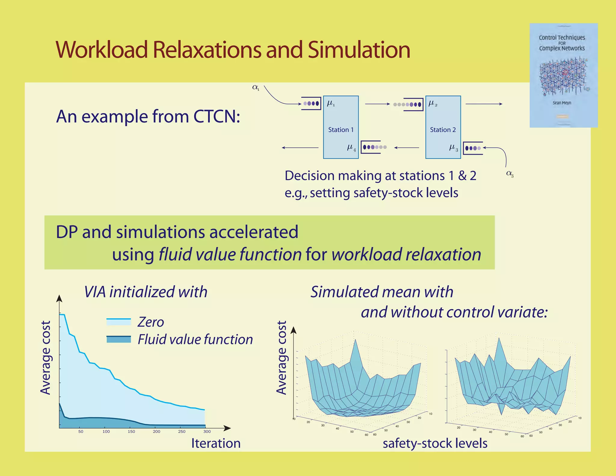
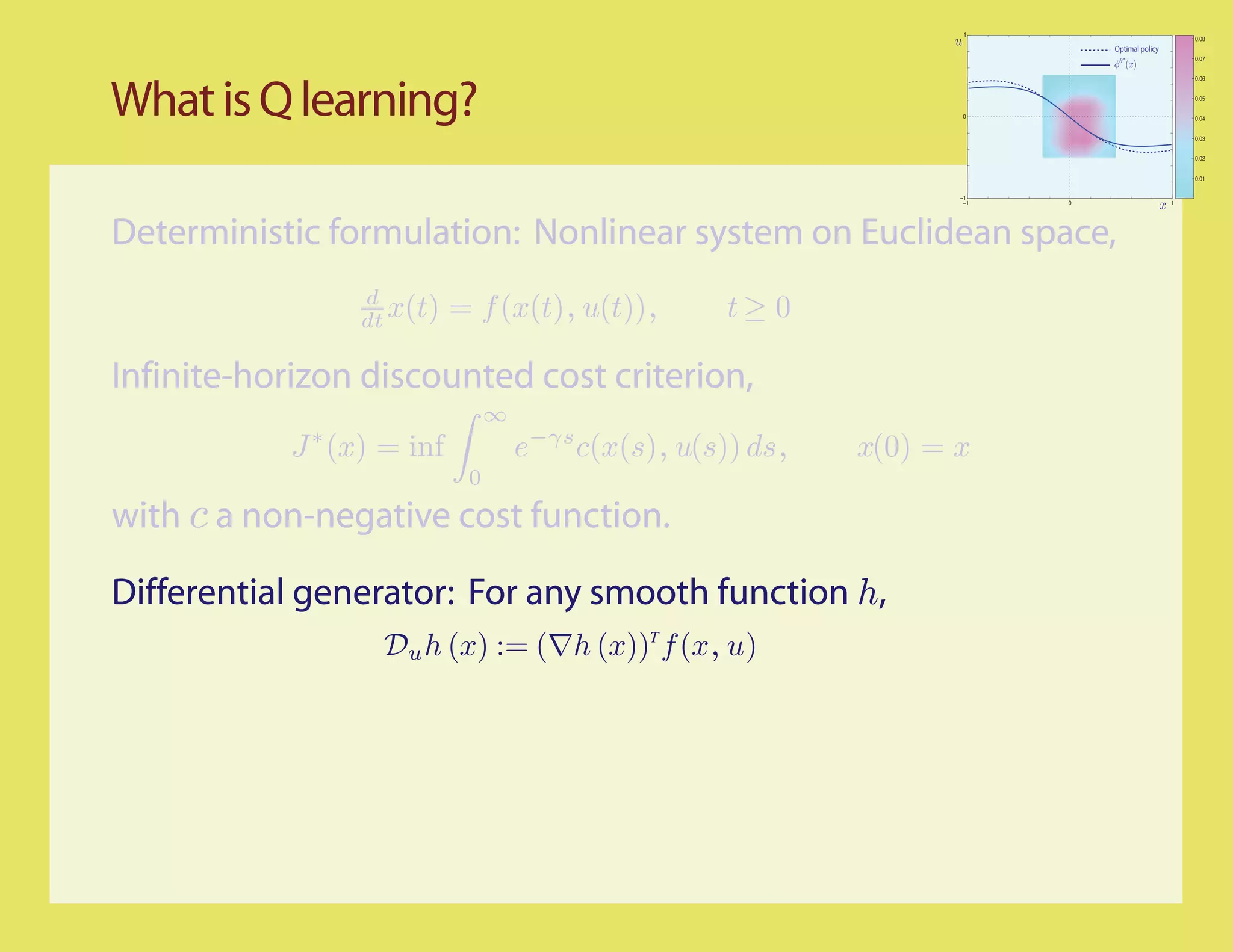
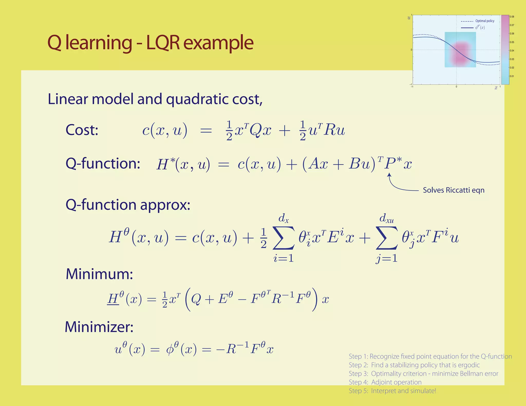
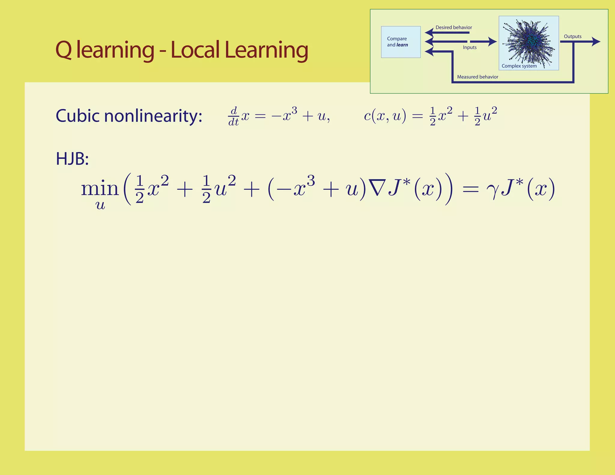
Step 2: Stationary policy that is ergodic?
Suppose for example the input is scalar, and the system is stable
[Bounded-input/Bounded-state]
Can try a linear
combination
of sinusouids
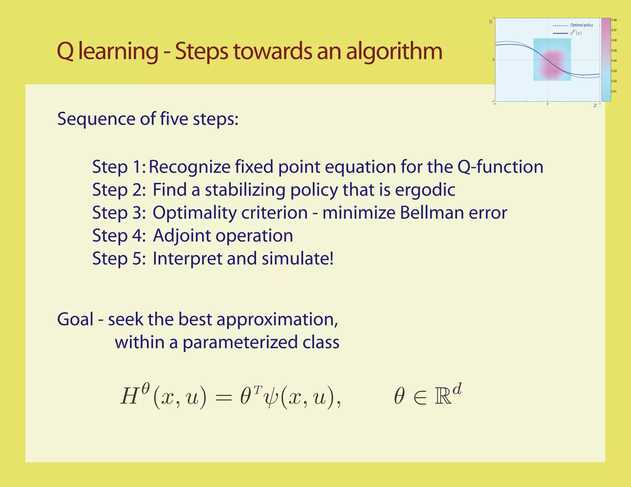
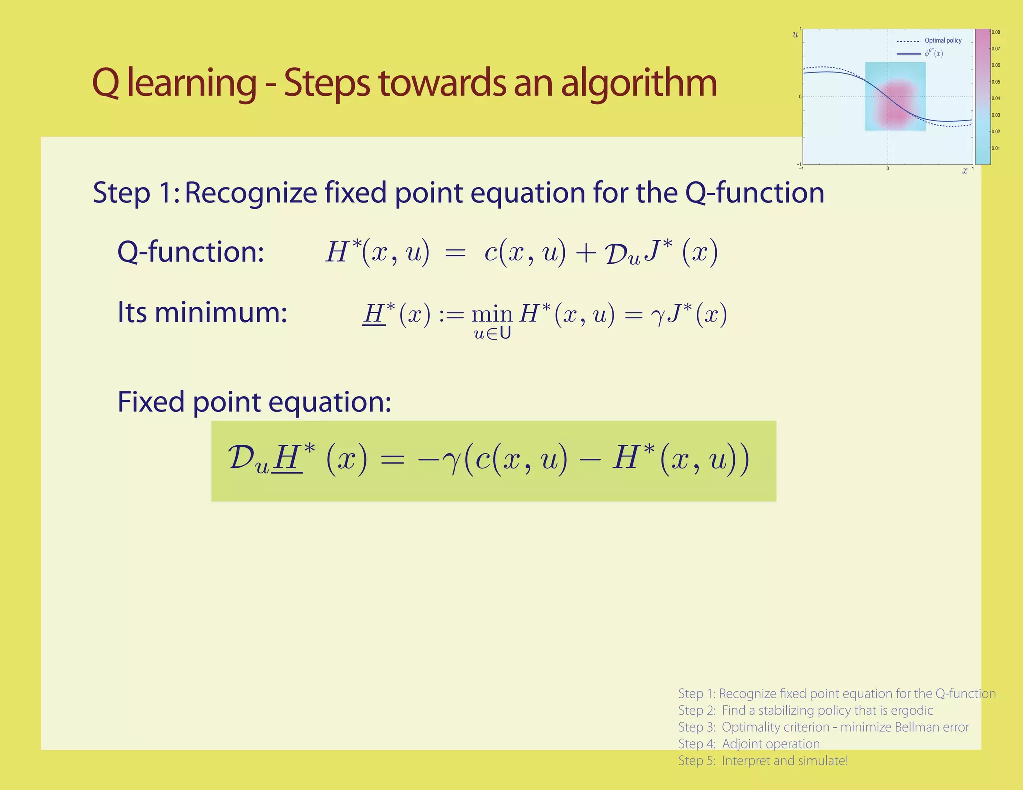
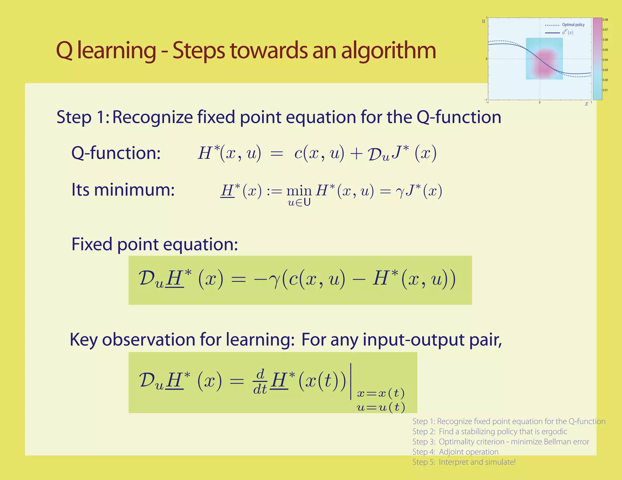
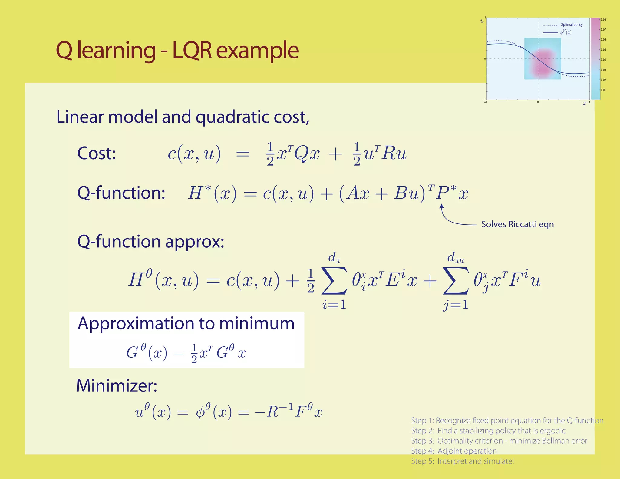
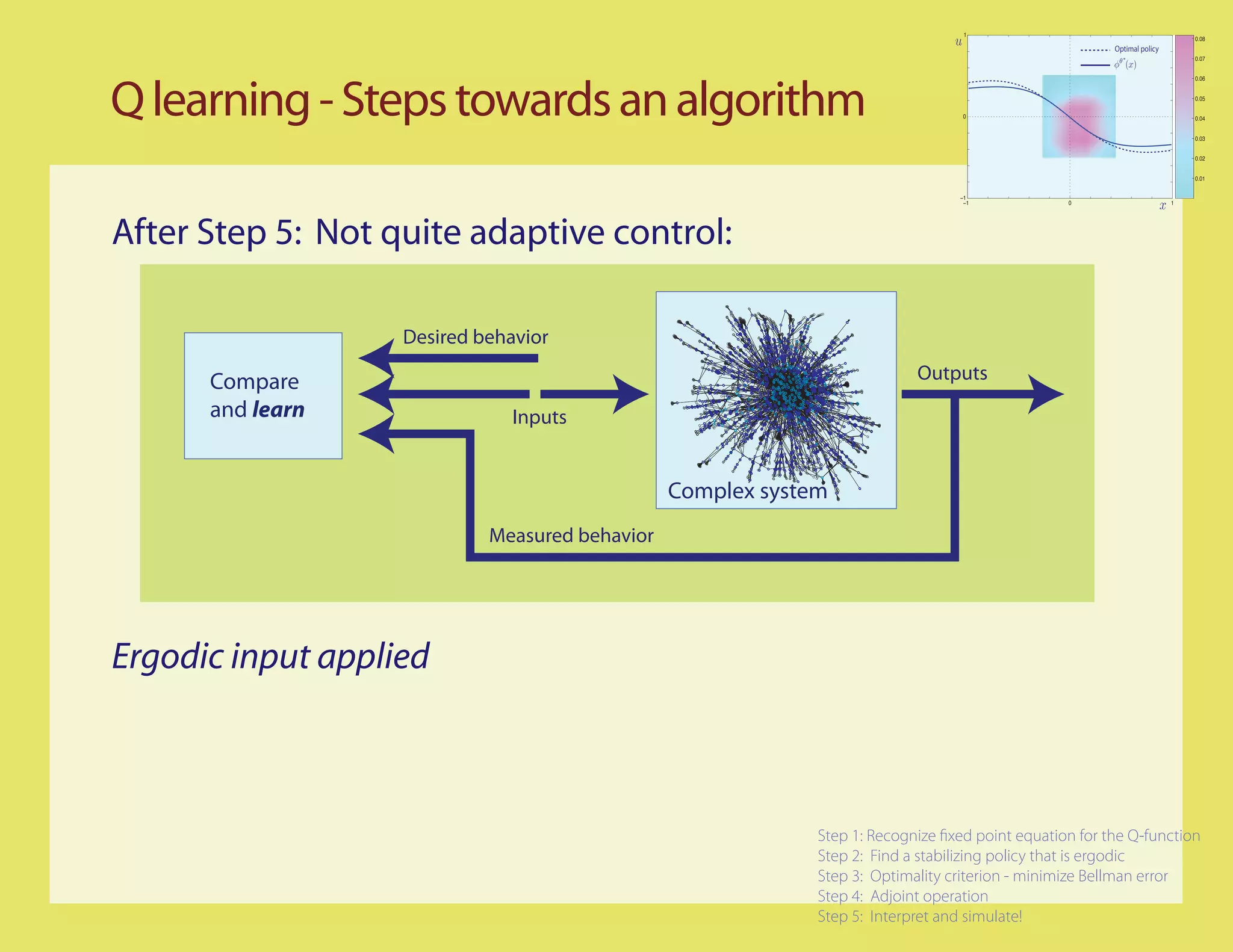
Step 1: Recognize xed point equation for the Q-function
Step 2: Find a stabilizing policy that is ergodic
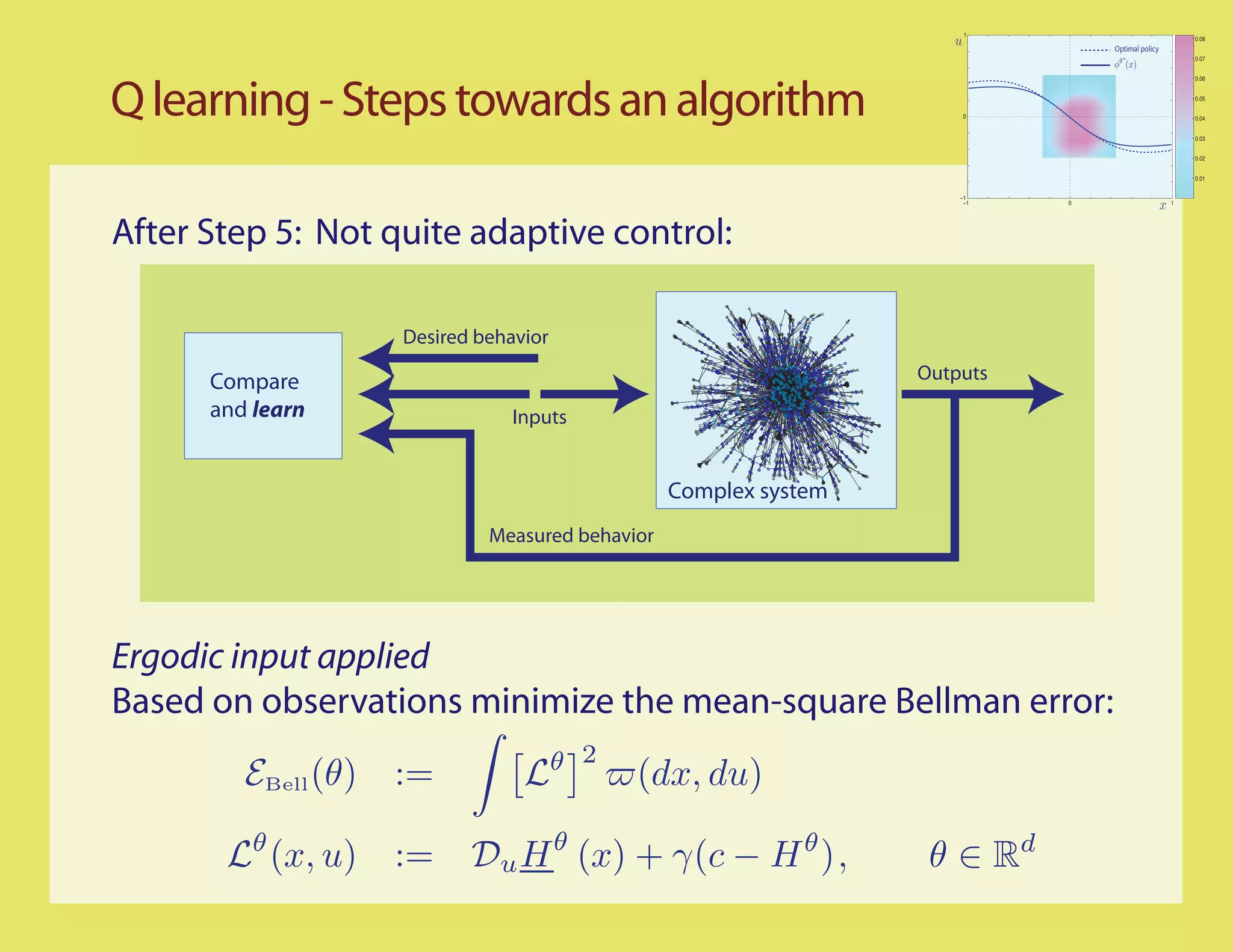
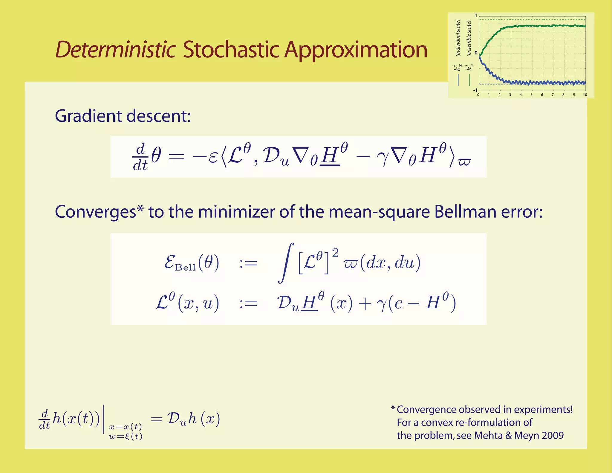
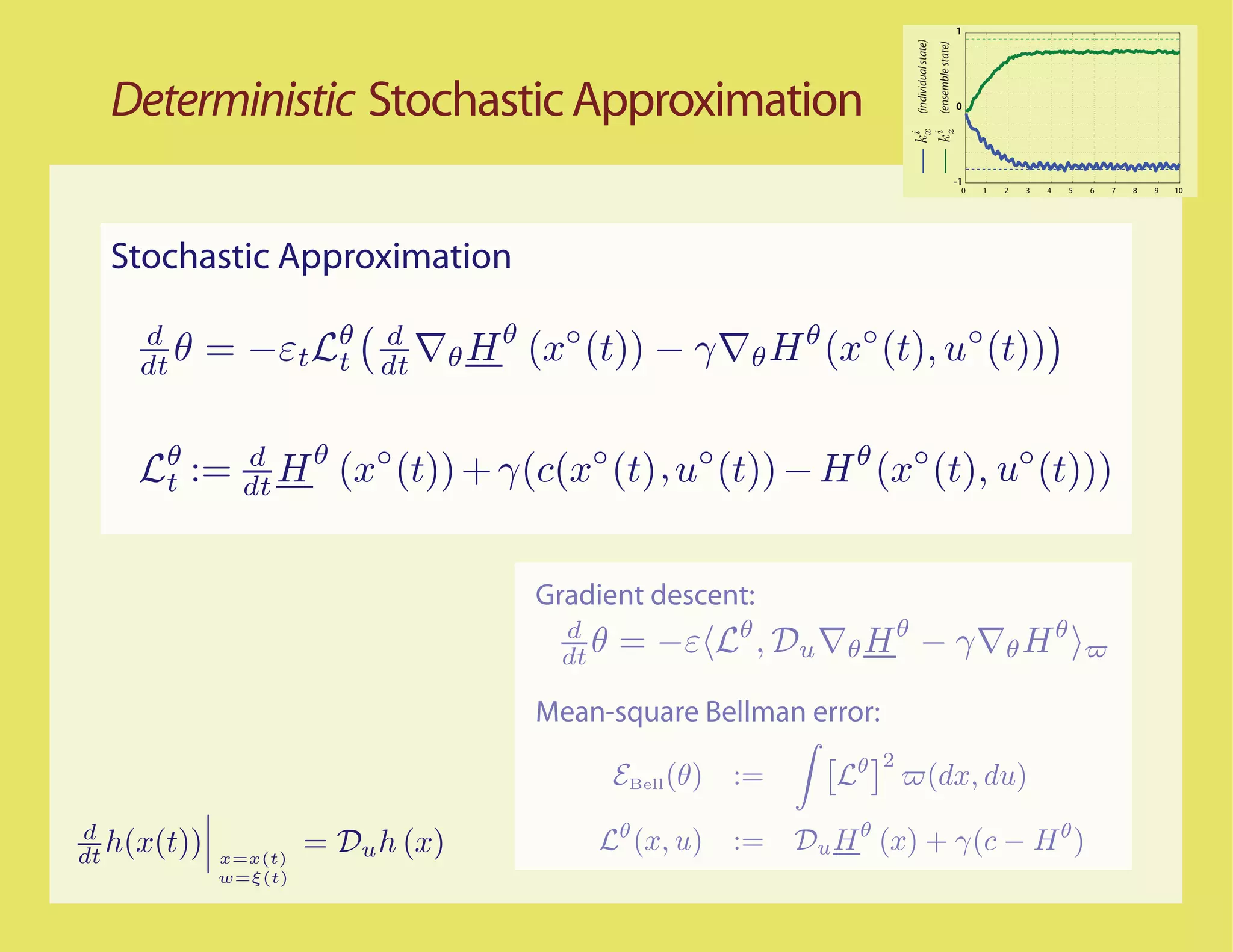
Step 3: Optimality criterion - minimize Bellman error
Step 4: Adjoint operation
Step 5: Interpret and simulate!](https://image.slidesharecdn.com/q-csl-may6-090919070038-phpapp01/75/Q-Learning-and-Pontryagin-s-Minimum-Principle-22-2048.jpg)
![1
0.08
Optimal policy
0.07
0.06
Q learning - Steps towards an algorithm 0
0.05
0.04
0.03
0.02
0.01
−1
−1 0 1
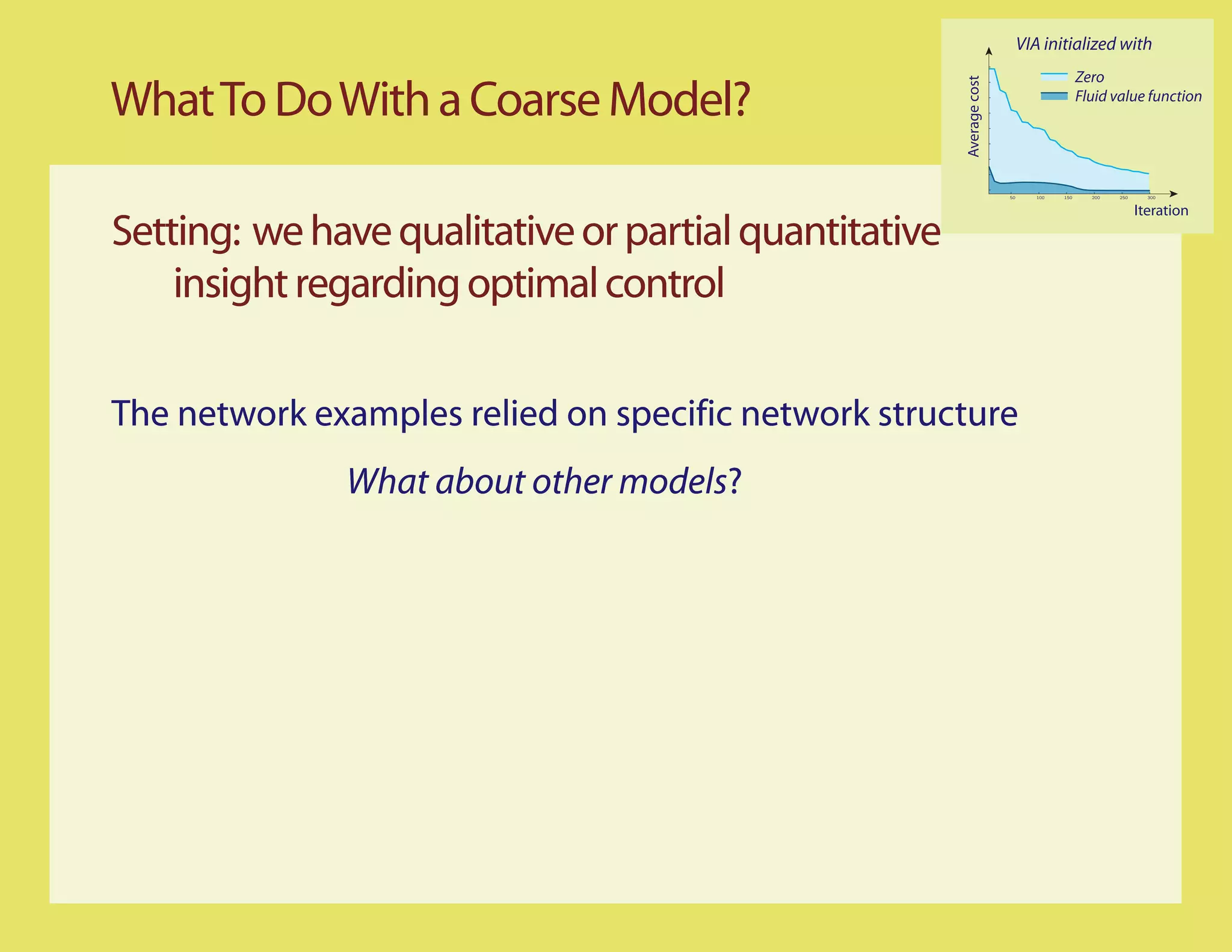
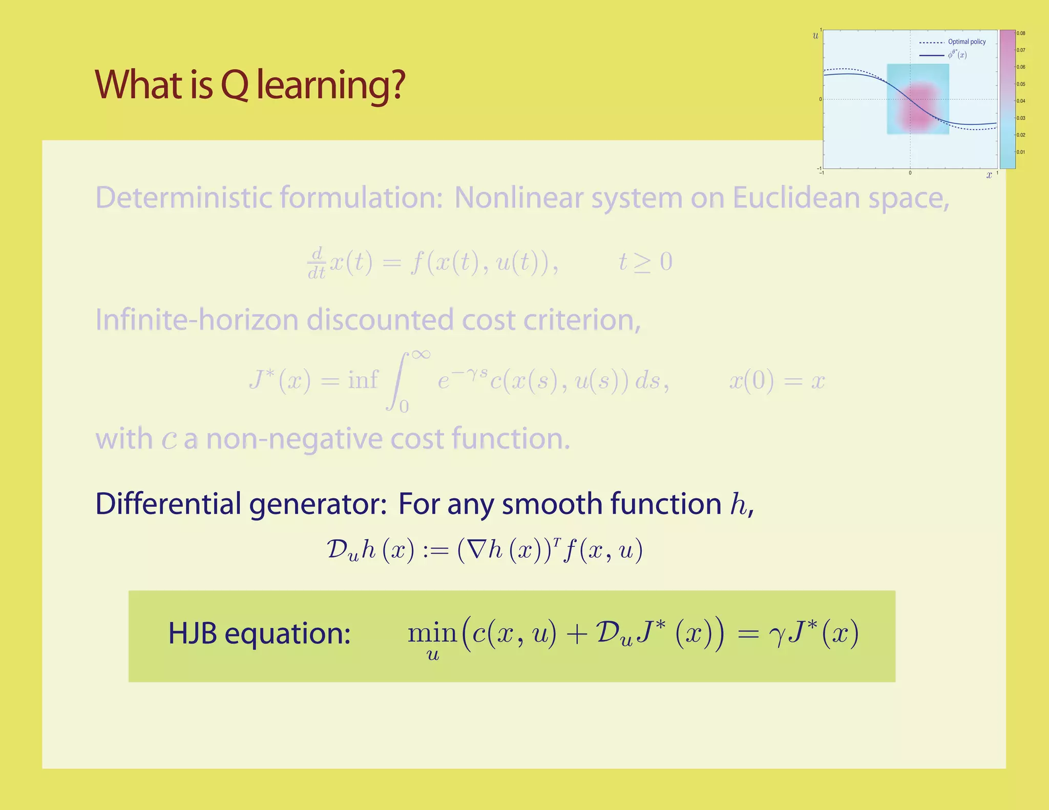
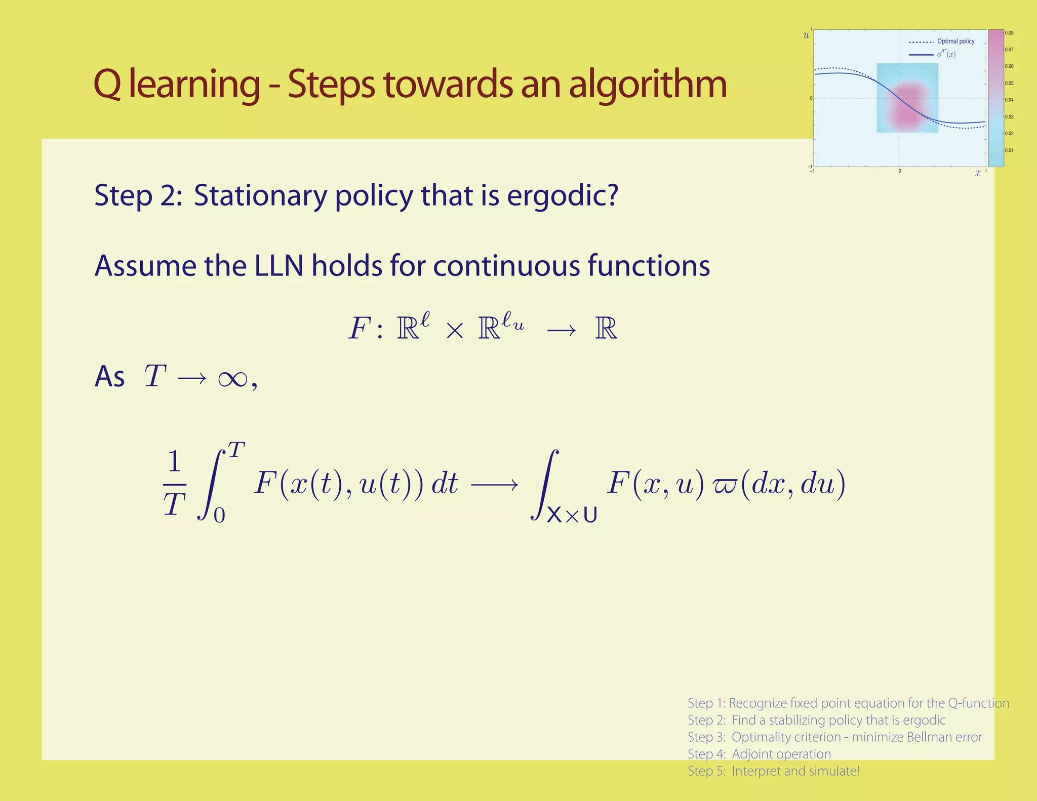
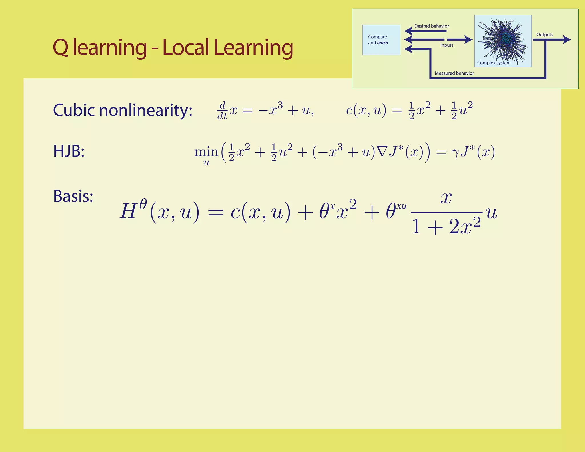
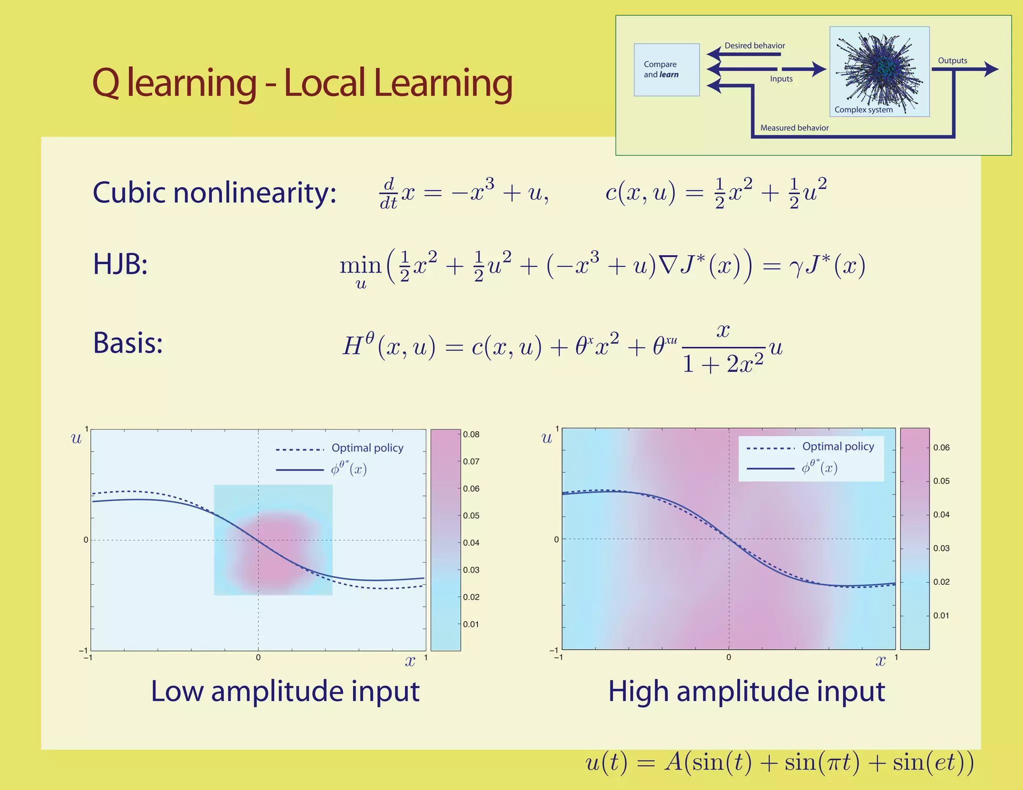
Step 2: Stationary policy that is ergodic?
Suppose for example the input is scalar, and the system is stable
[Bounded-input/Bounded-state]
0.08
0.07
0.06
0.05
Can try a linear
combination
0.04
of sinusouids
0.03
0.02
0.01
Step 1: Recognize xed point equation for the Q-function
u(t) = A(sin(t) + sin(πt) + sin(et)) Step 2: Find a stabilizing policy that is ergodic
Step 3: Optimality criterion - minimize Bellman error
Step 4: Adjoint operation
Step 5: Interpret and simulate!](https://image.slidesharecdn.com/q-csl-may6-090919070038-phpapp01/75/Q-Learning-and-Pontryagin-s-Minimum-Principle-23-2048.jpg)
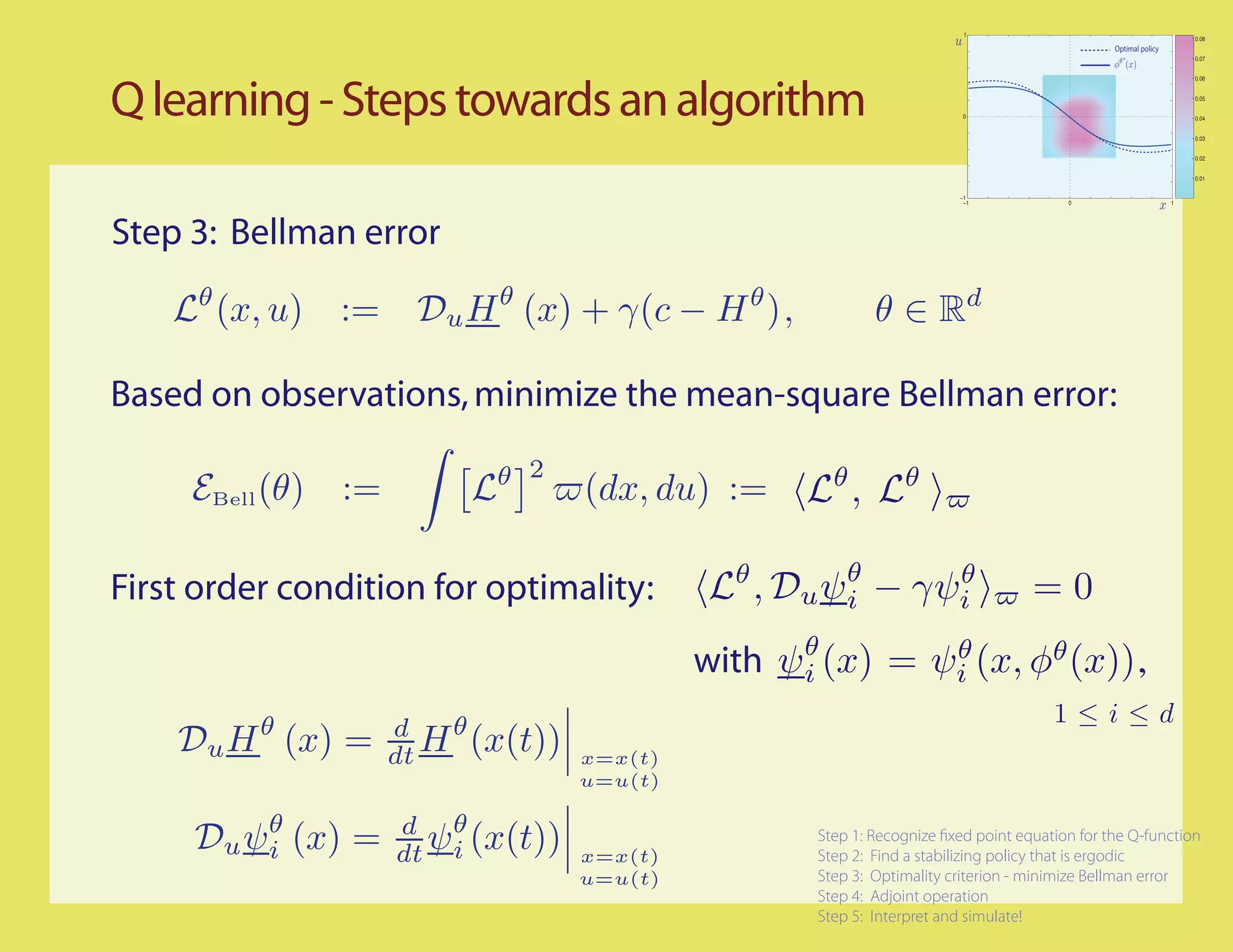
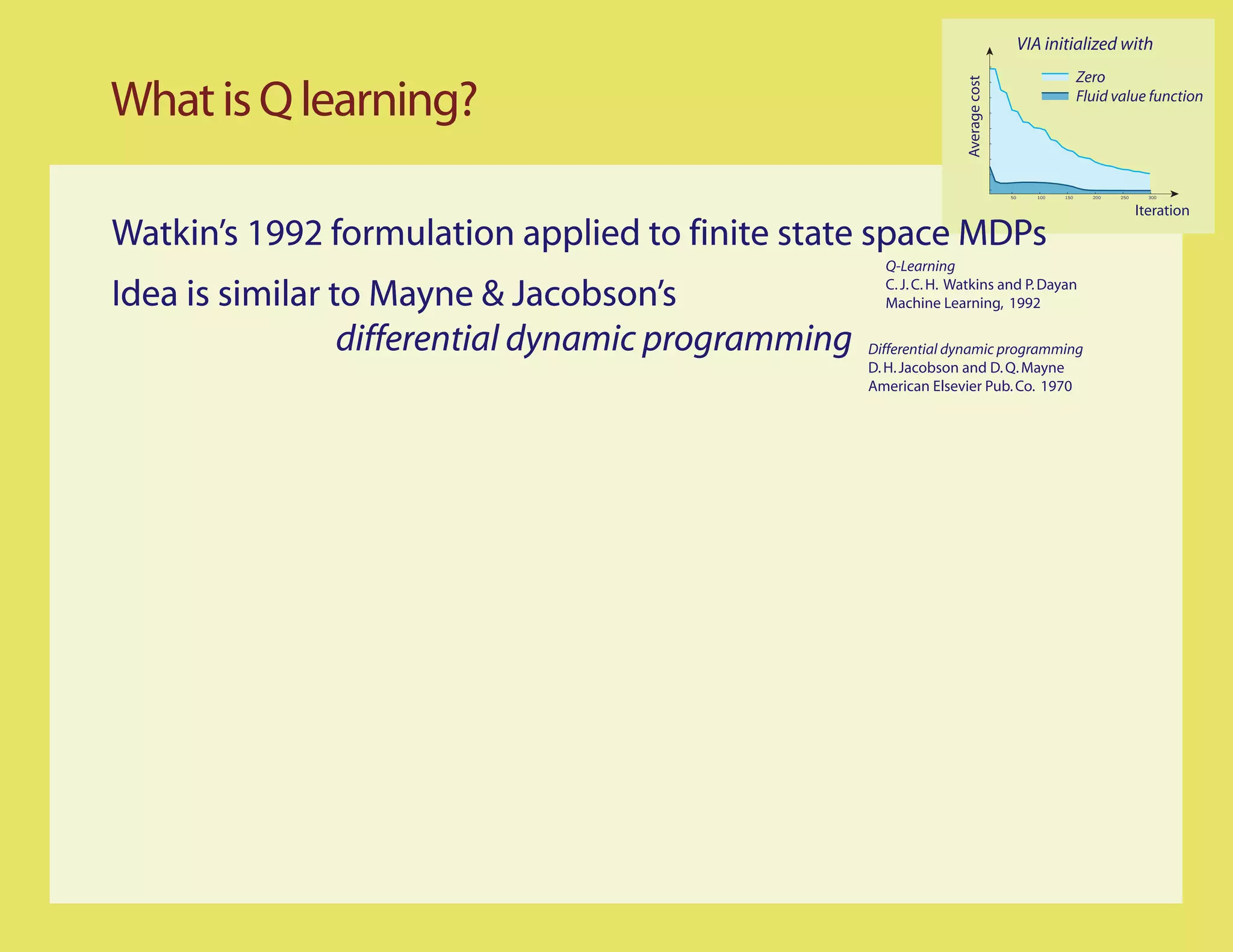
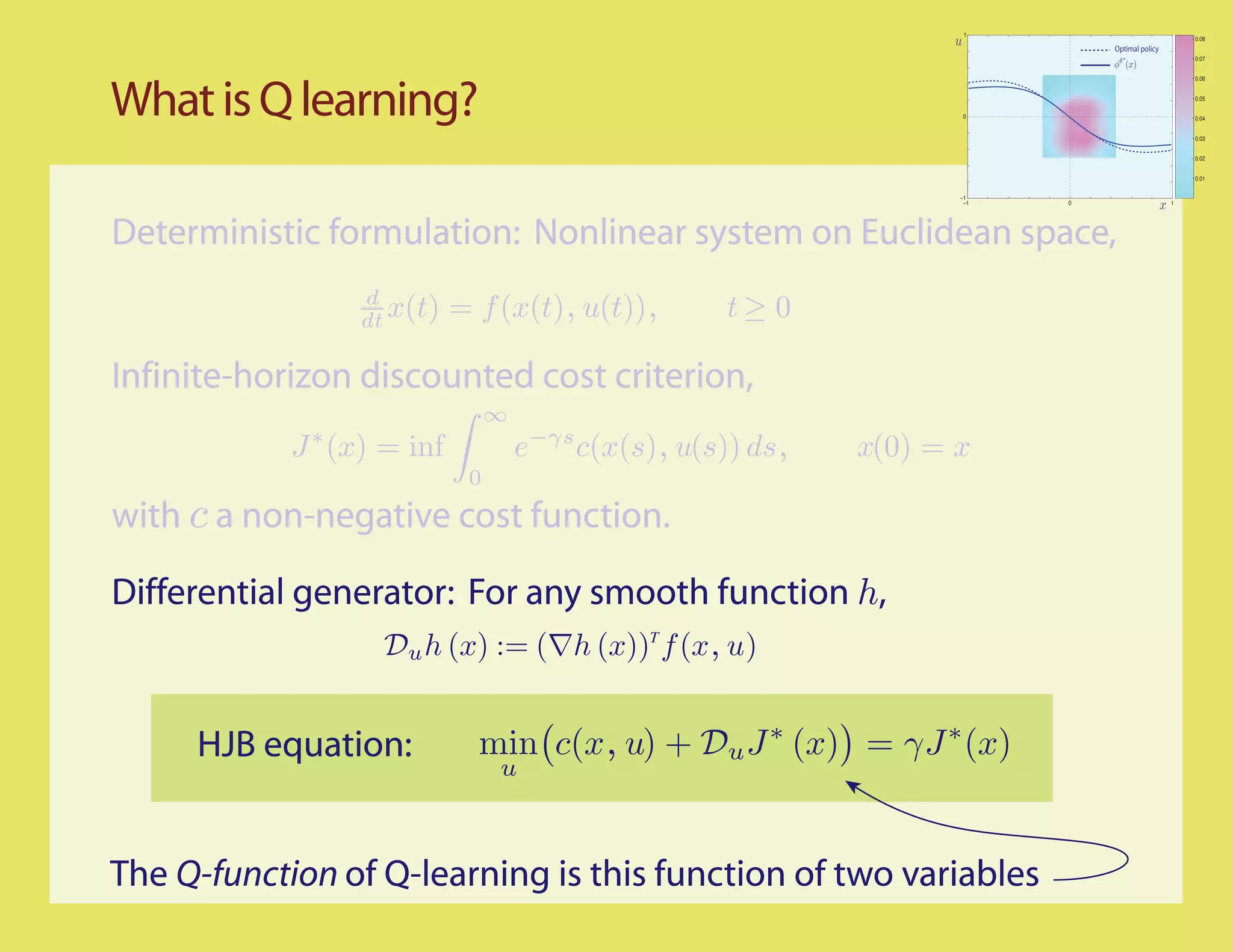
![Q learning - Steps towards an algorithm
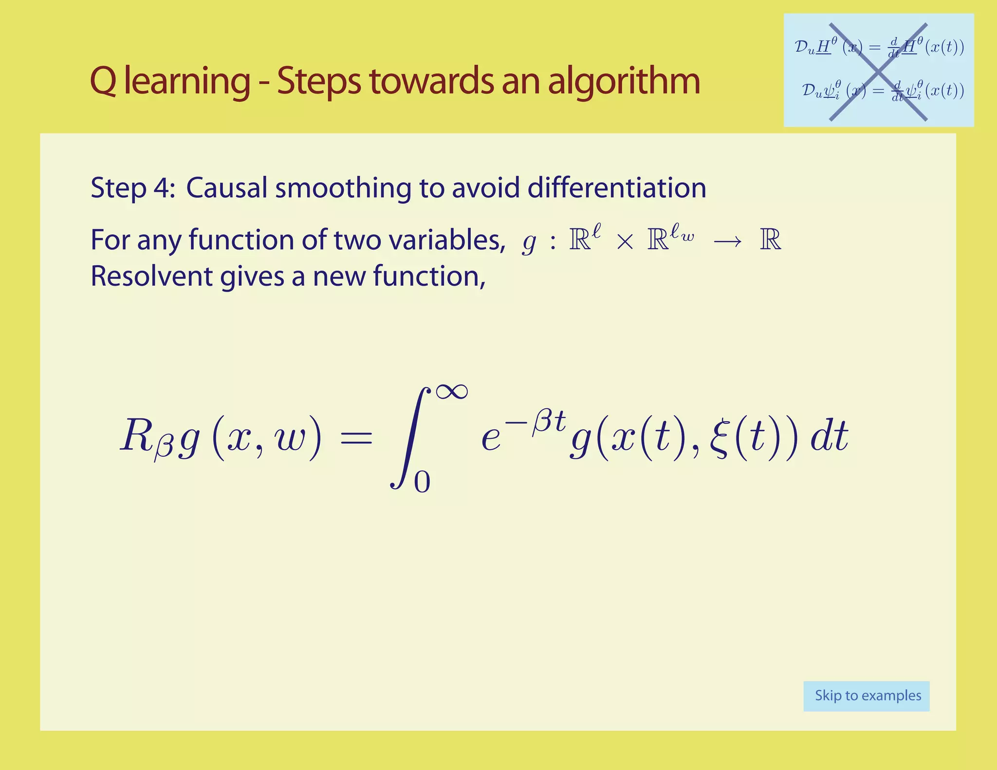
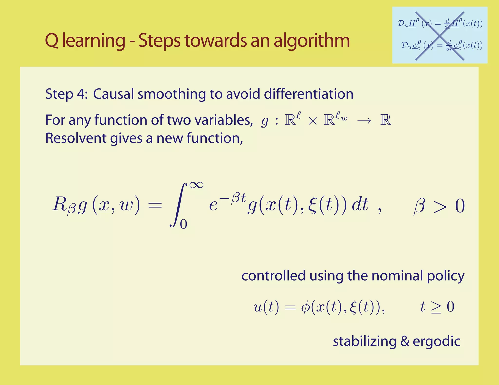
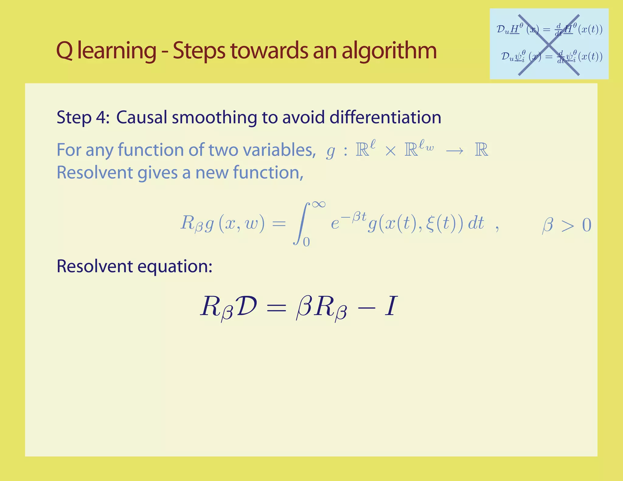
Step 4: Causal smoothing to avoid differentiation
For any function of two variables, g : R × R w
→ R
Resolvent gives a new function,
∞
Rβ g (x, w) = e−βt g(x(t), ξ (t)) dt , β>0
0
Resolvent equation:
Smoothed Bellman error:
Lθ,β = Rβ Lθ
θ θ
= [βRβ − I]H + γRβ (c − H )](https://image.slidesharecdn.com/q-csl-may6-090919070038-phpapp01/75/Q-Learning-and-Pontryagin-s-Minimum-Principle-30-2048.jpg)
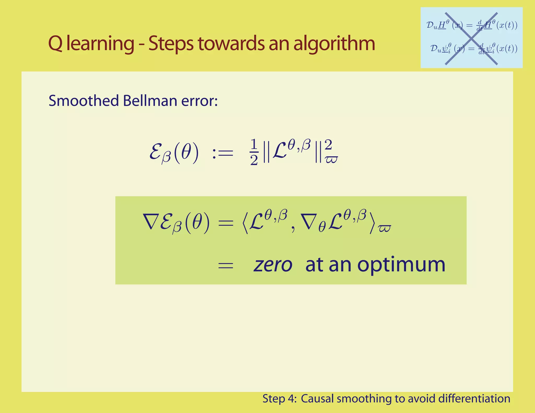
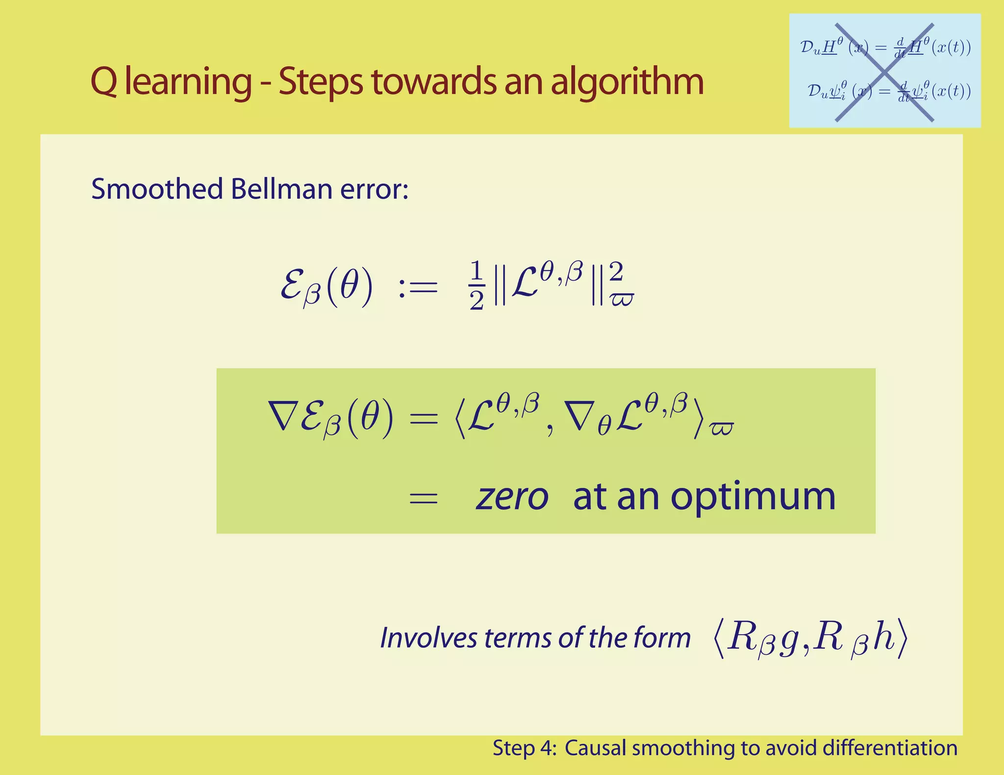
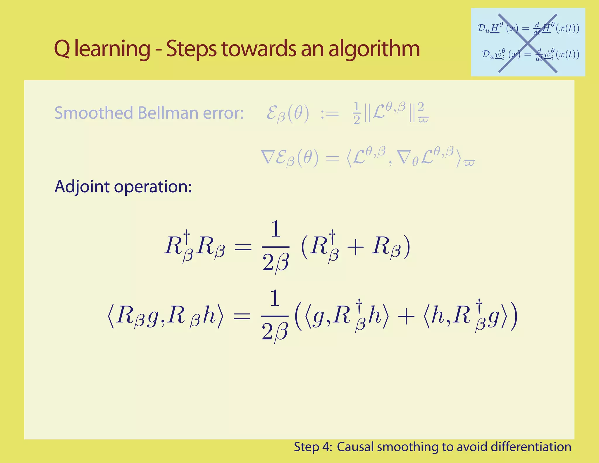
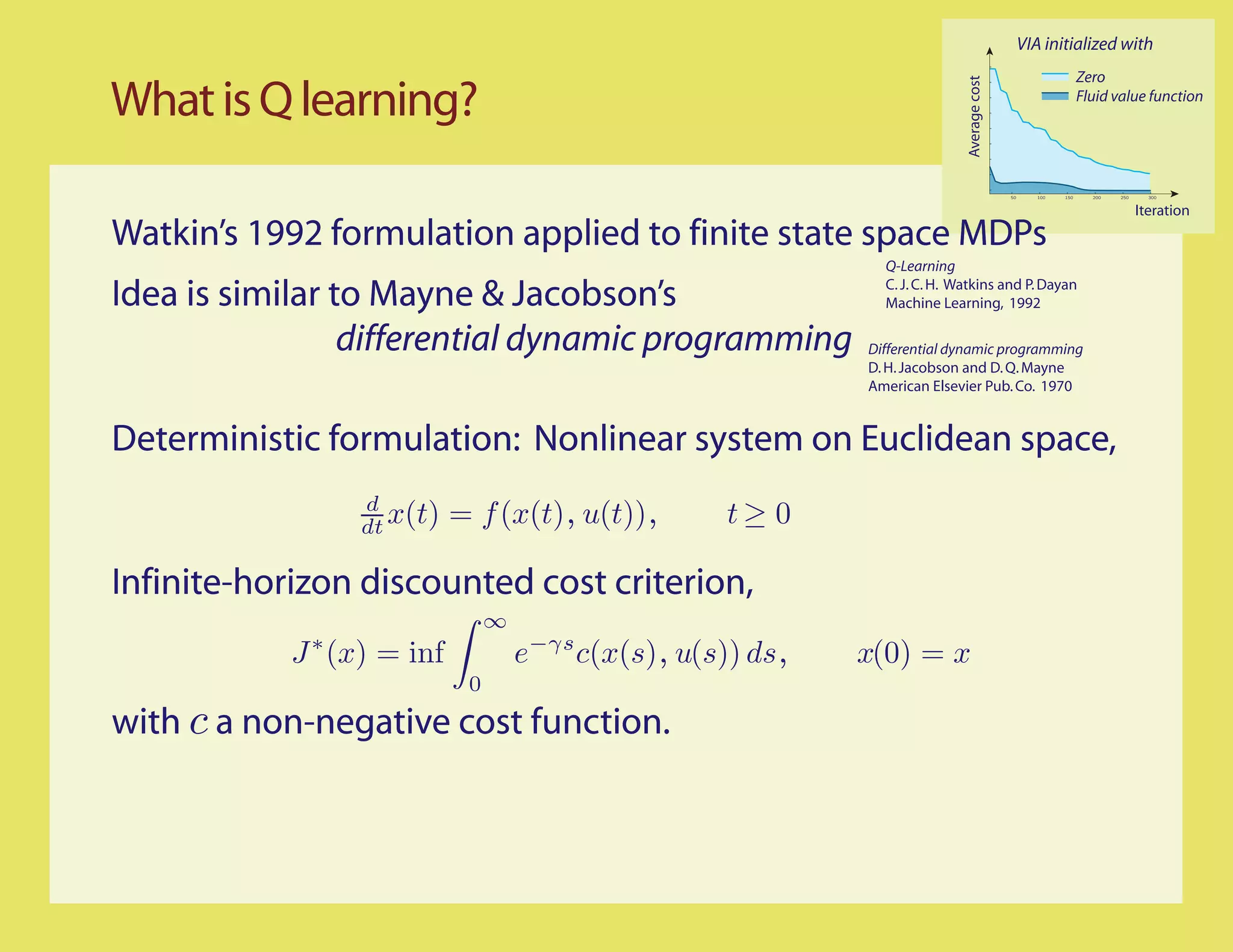
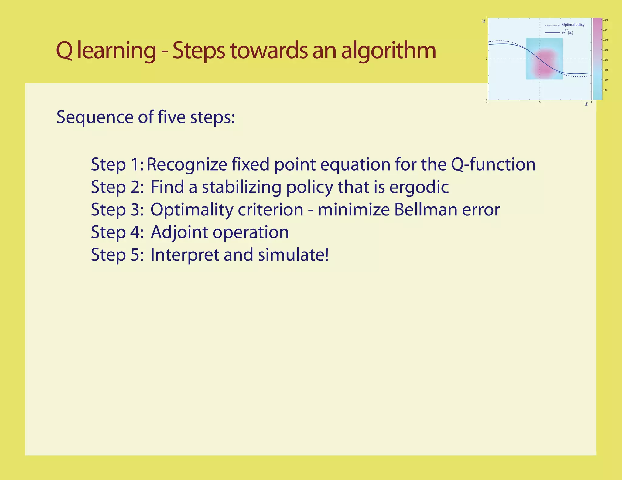
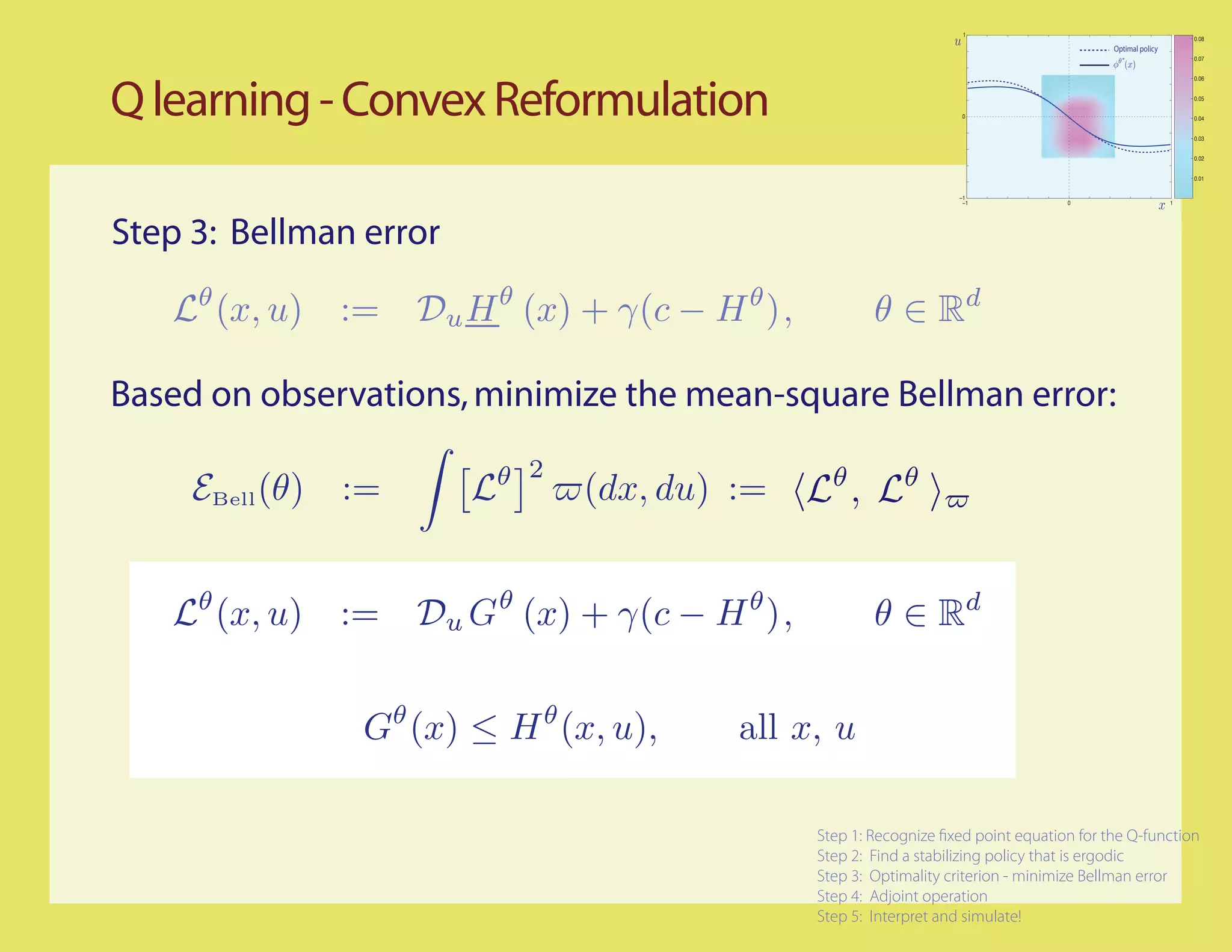
![Q learning - Steps towards an algorithm
1 θ,β 2
Smoothed Bellman error: Eβ (θ) := 2
θ,β θ,β
Eβ (θ) = , θL
Adjoint operation: 1
† †
Rβ Rβ = (Rβ + Rβ )
2β
1 † †
Rβ g,R β h = g,R β h + h,R β g
2β
Adjoint realization: time-reversal
∞
†
Rβ g (x, w) = e−βt Ex, w [g(x◦ (−t), ξ ◦ (−t))] dt
0
expectation conditional on x◦ (0) = x, ξ ◦ (0) = w.
Step 4: Causal smoothing to avoid differentiation](https://image.slidesharecdn.com/q-csl-may6-090919070038-phpapp01/75/Q-Learning-and-Pontryagin-s-Minimum-Principle-34-2048.jpg)


![References
.
PhD thesis, University of London, London, England, 1967.
. American Elsevier Pub. Co., New York, NY, 1970.
Learning from Delayed Rewards. PhD thesis, King’s College, Cambridge, UK, 1989.
Machine Learning, 8(3-4):279–292, 1992.
SIAM J. Control Optim., 38(2):447–469, 2000.
on policy iteration. Automatica, 45(2):477 – 484, 2009.
Submitted to the 48th IEEE Conference on Decision and Control, December 16-18 2009.
[9] C. Moallemi, S. Kumar, and B. Van Roy. Approximate and data-driven dynamic programming for queueing networks.
Preprint available at http://moallemi.com/ciamac/research-interests.php, 2008.](https://image.slidesharecdn.com/q-csl-may6-090919070038-phpapp01/75/Q-Learning-and-Pontryagin-s-Minimum-Principle-52-2048.jpg)

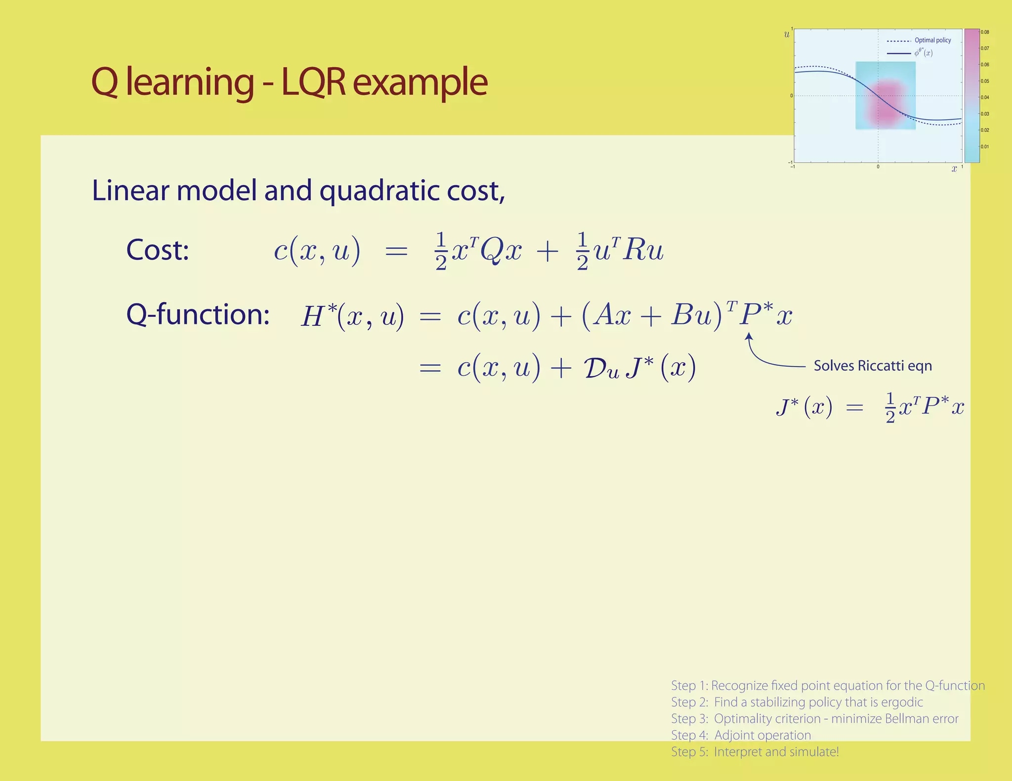
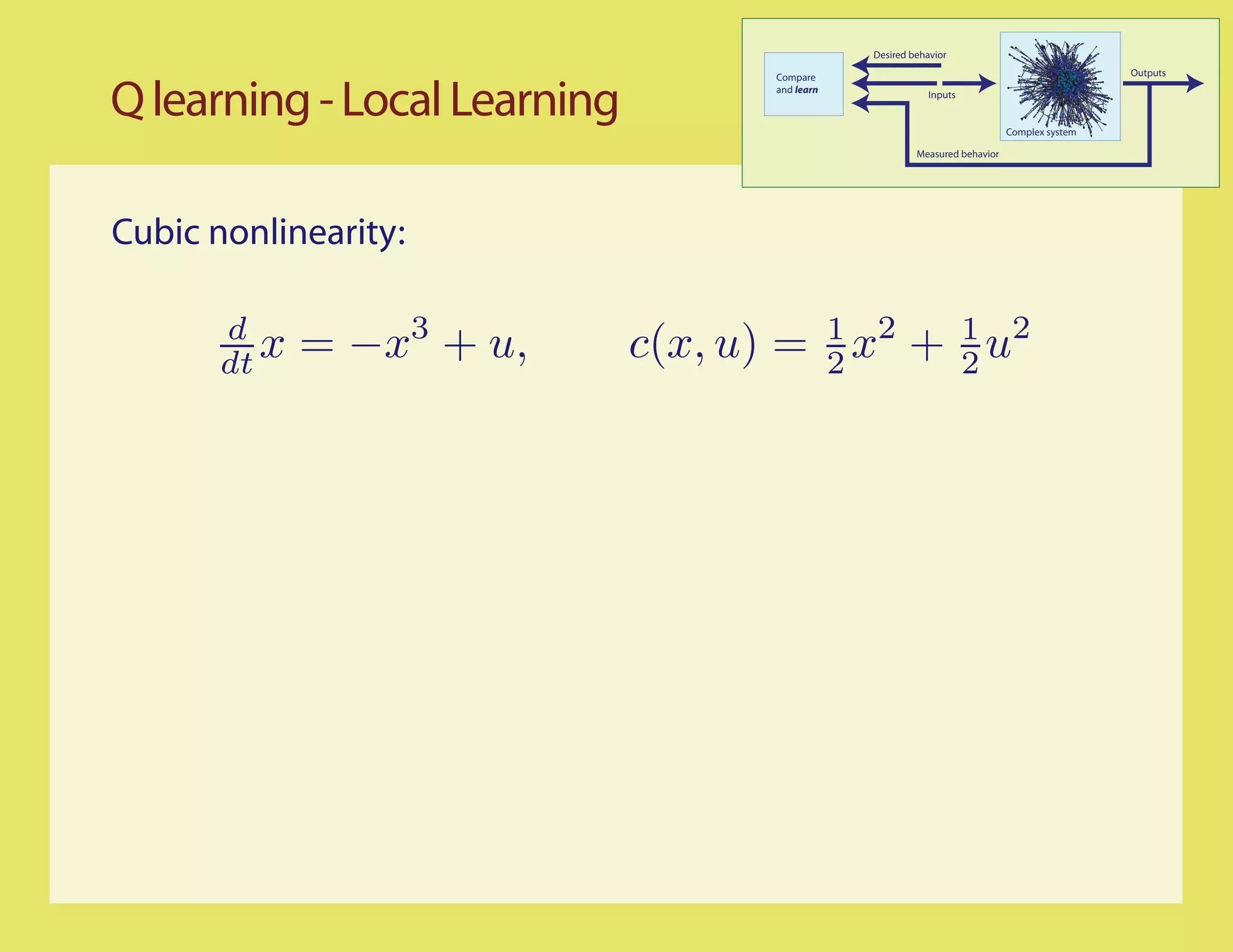
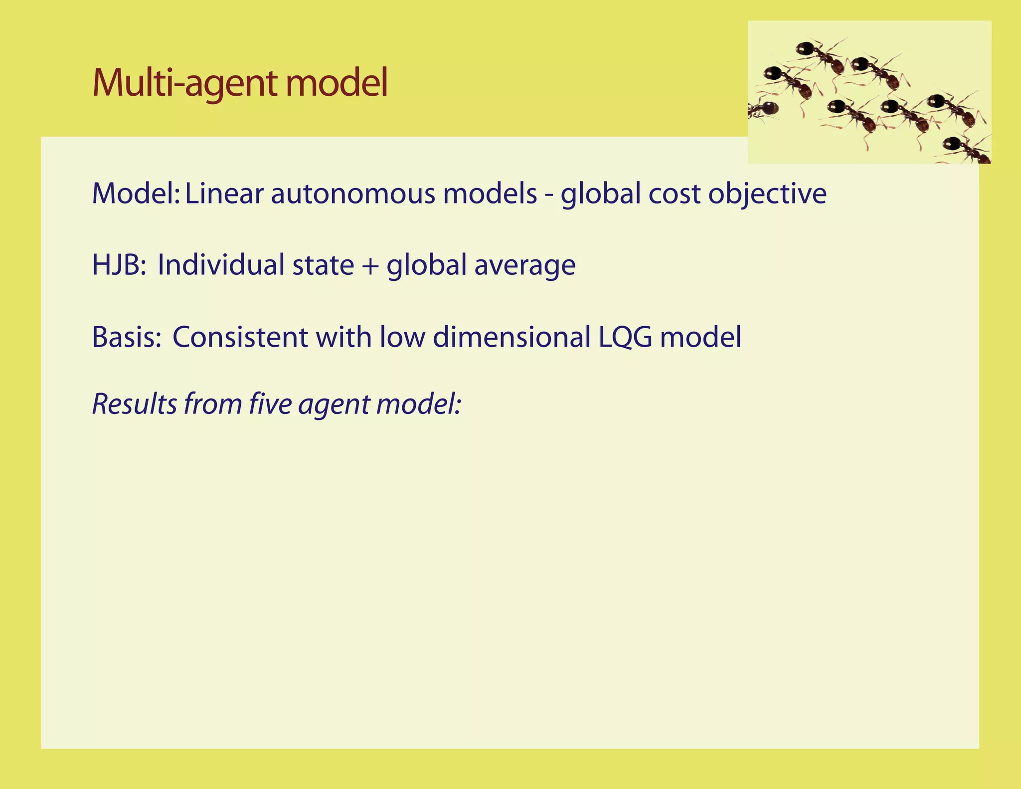
This document discusses using Q-learning to find optimal control policies for nonlinear systems with continuous state spaces. It outlines a 5-step approach: 1) Recognize the fixed point equation for the Q-function, 2) Find a stabilizing policy that is ergodic, 3) Use an optimality criterion to minimize the Bellman error, 4) Use an adjoint operation, and 5) Interpret and simulate the results. As an example, it applies these steps to the linear quadratic regulator (LQR) problem and approximates the Q-function. The goal is to seek the best approximation within a parameterized function class.