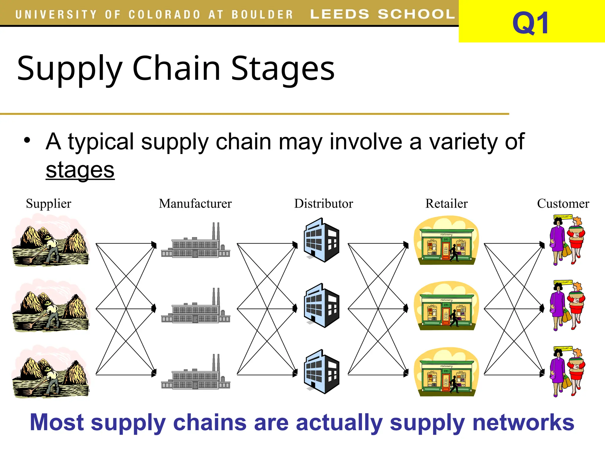
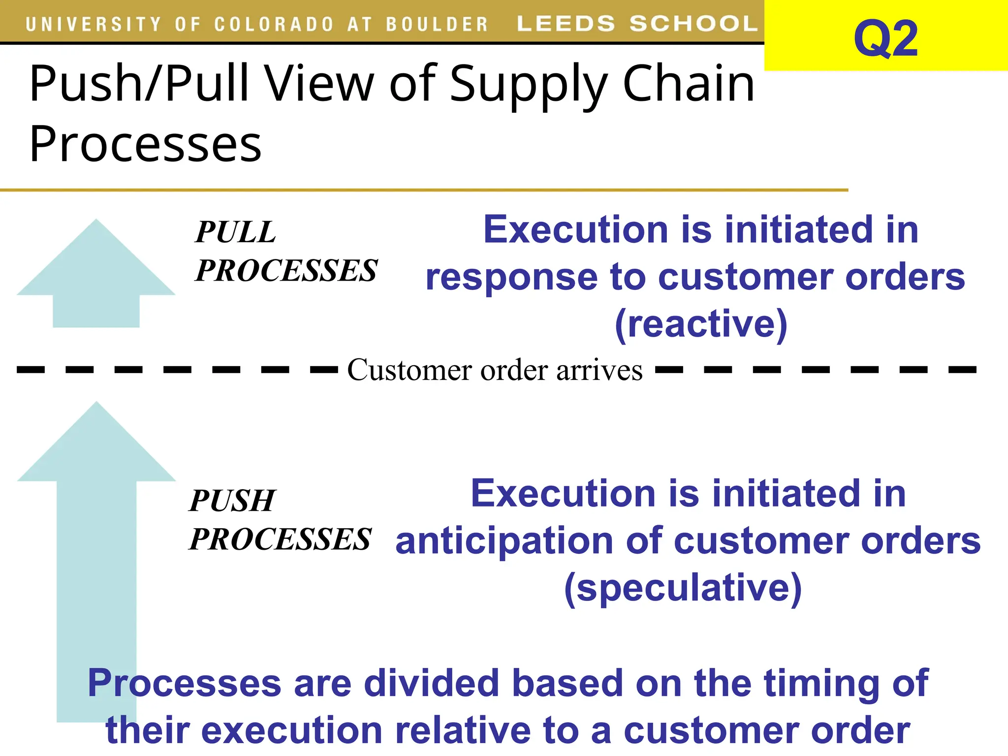
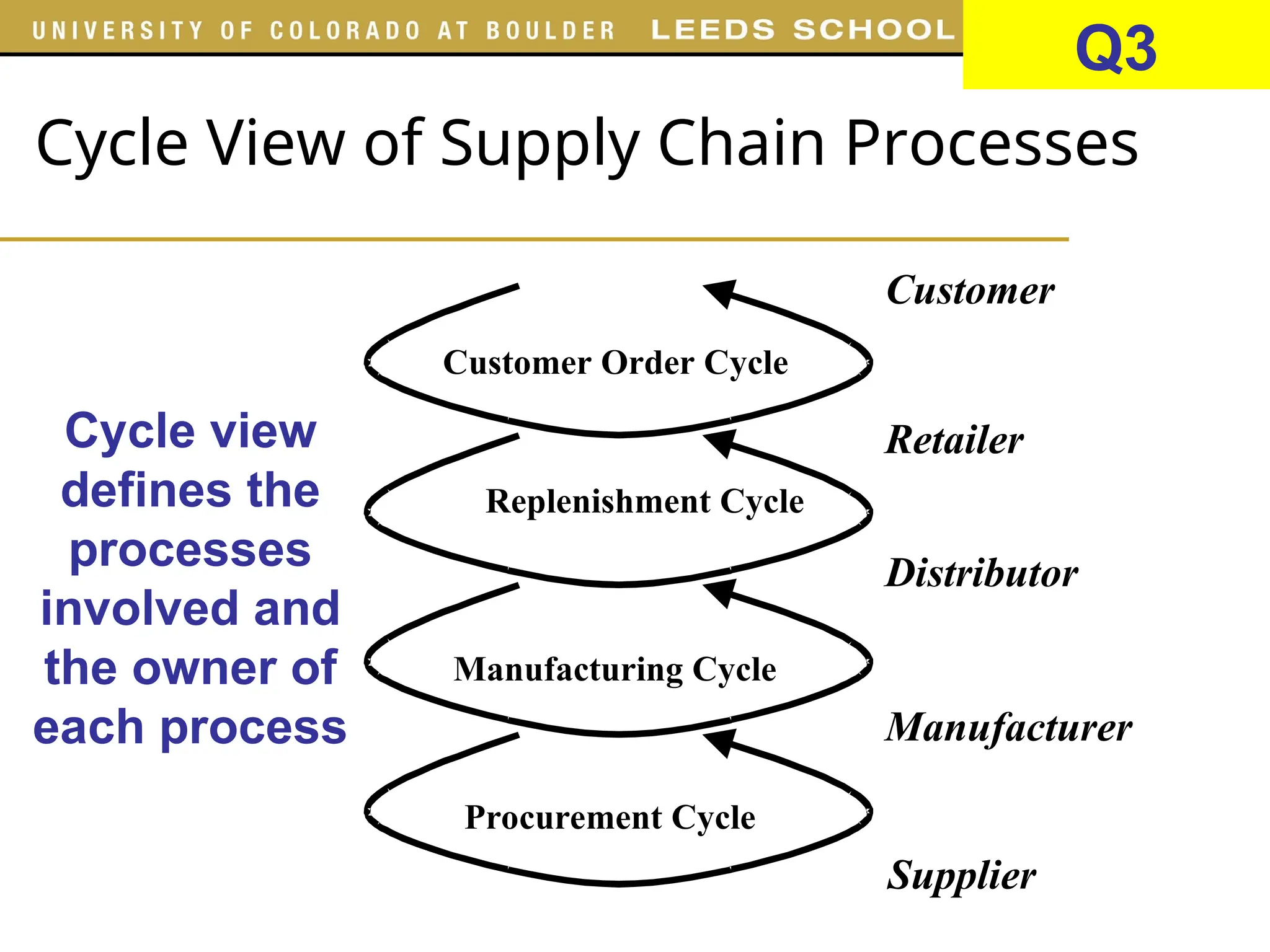
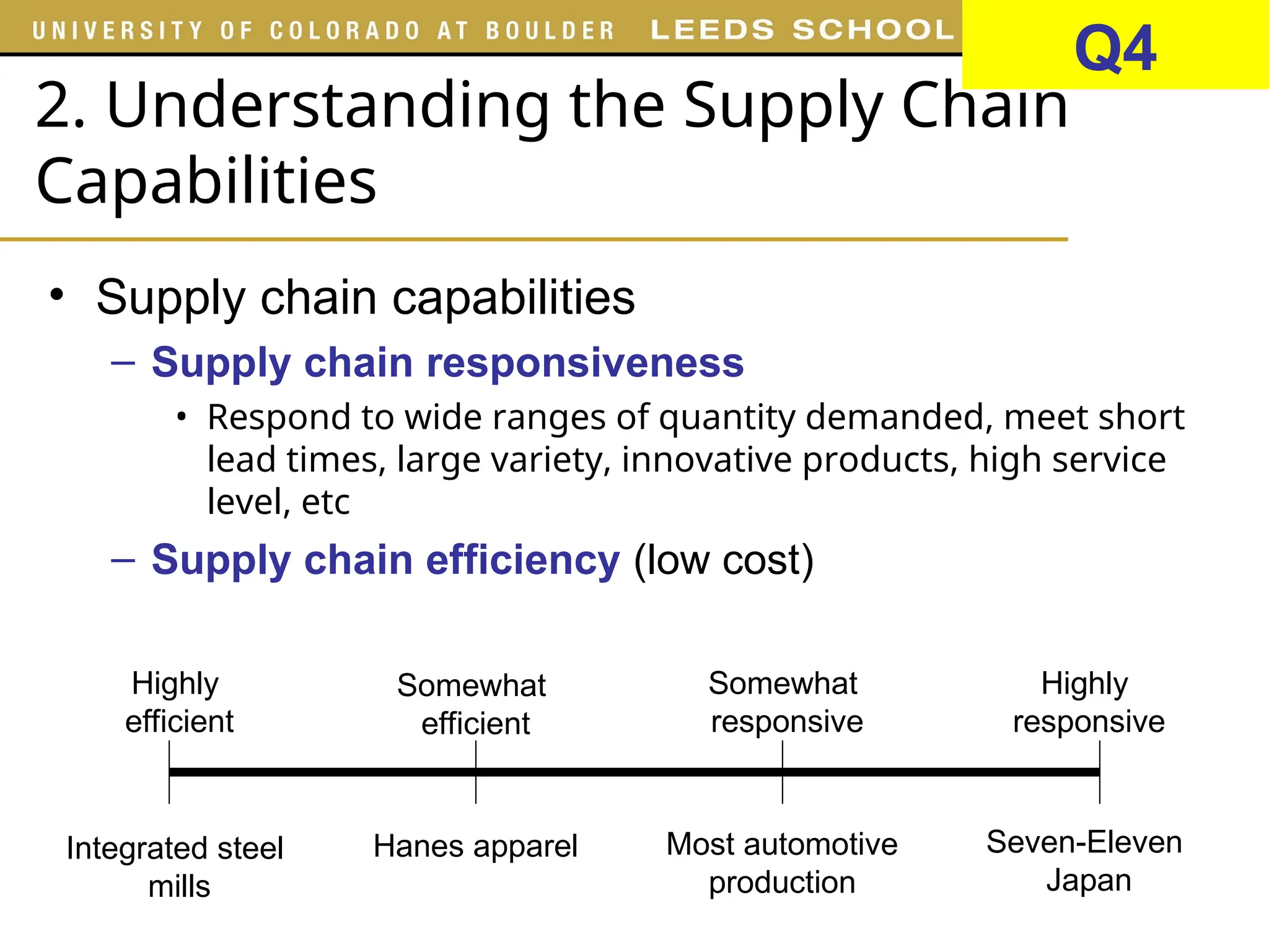
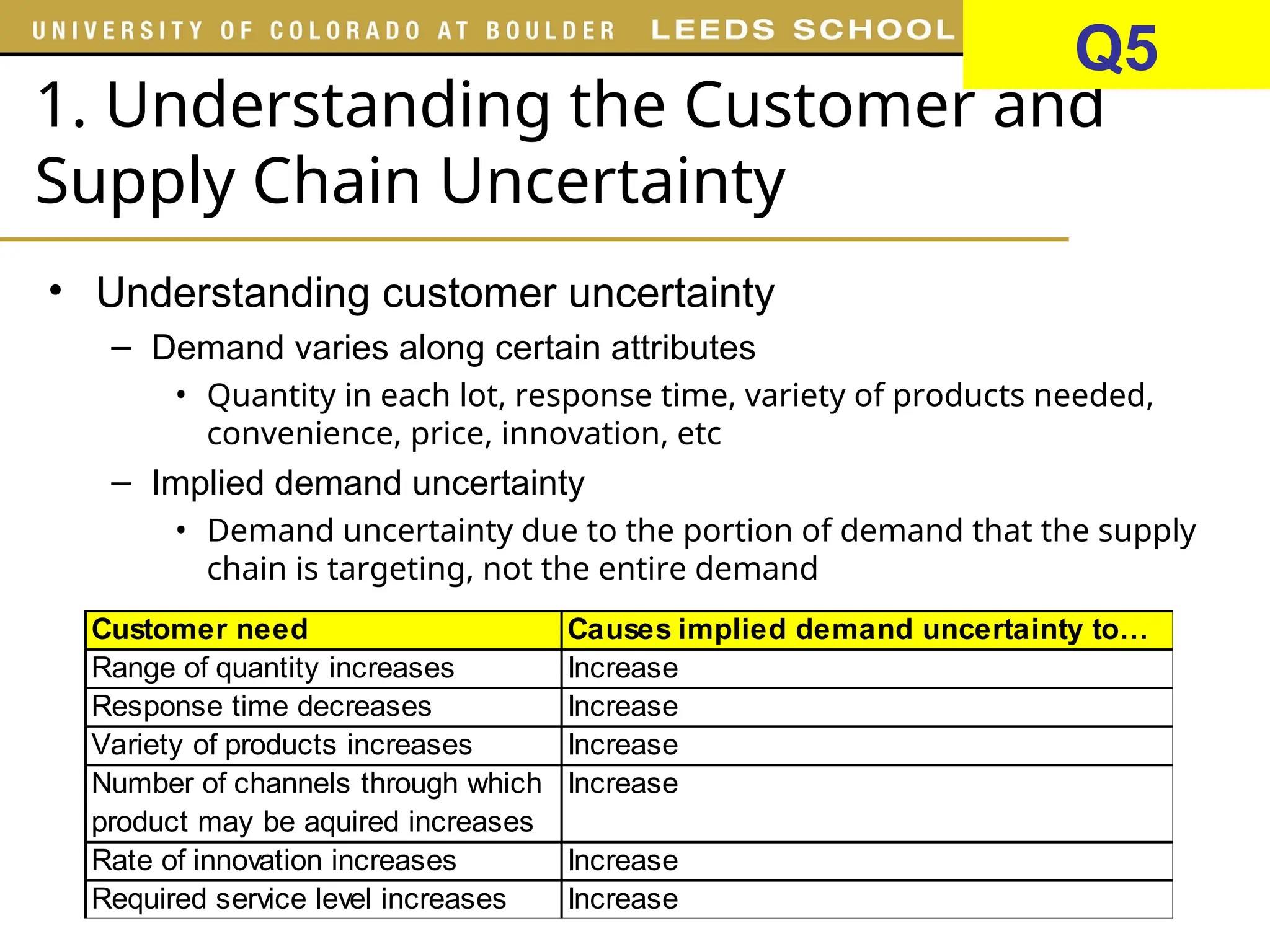
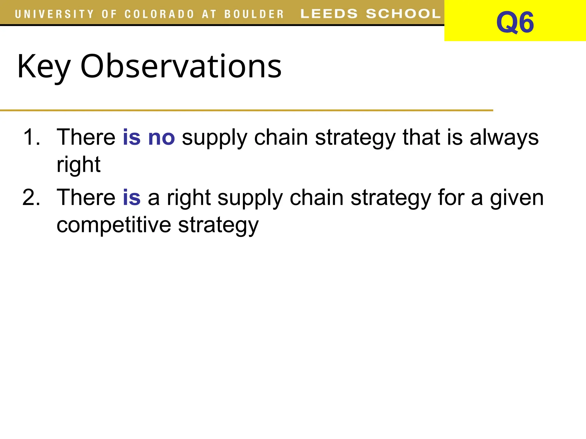
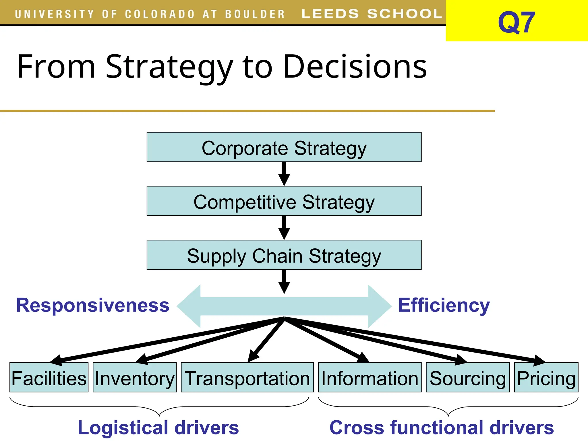
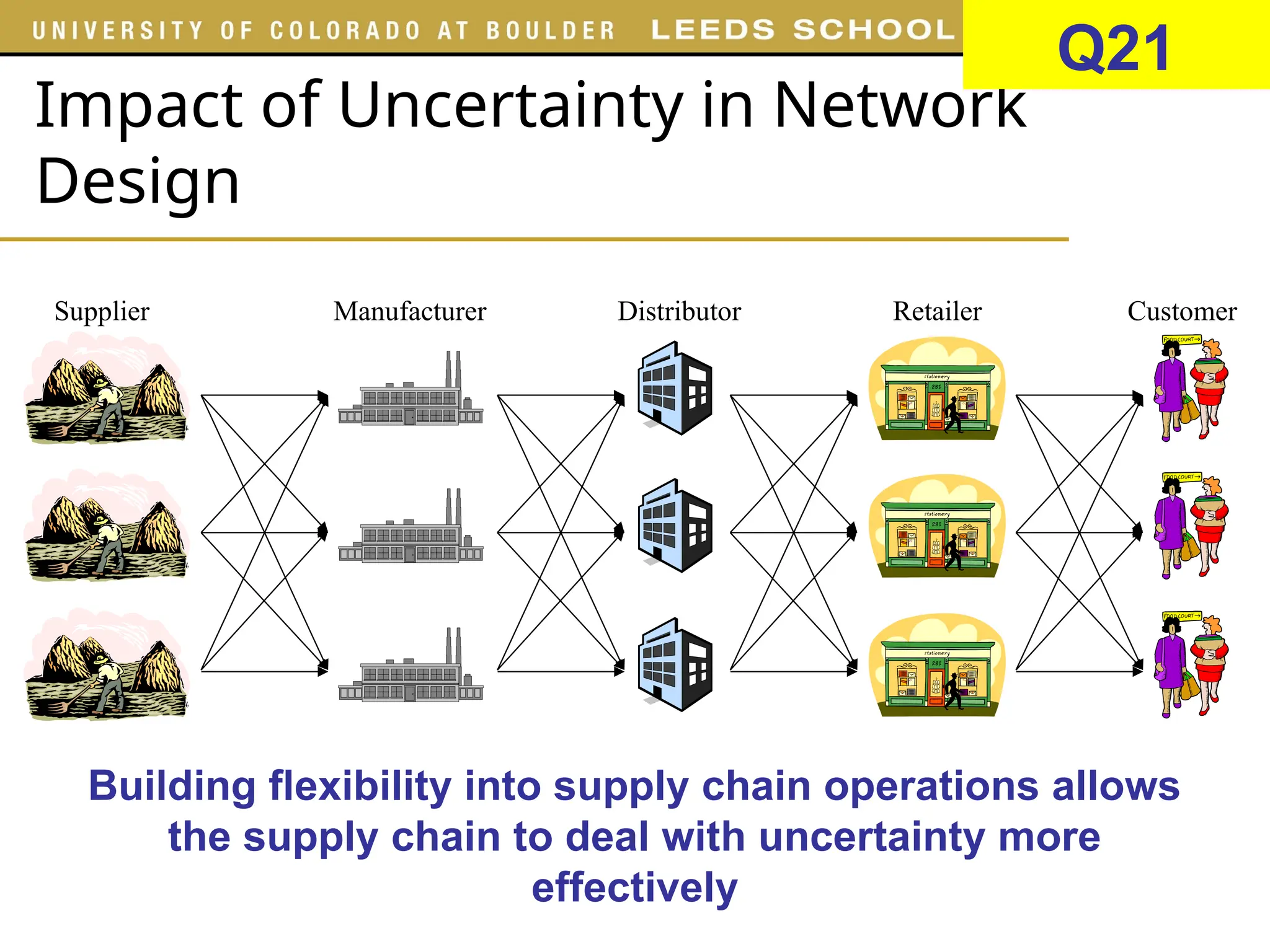
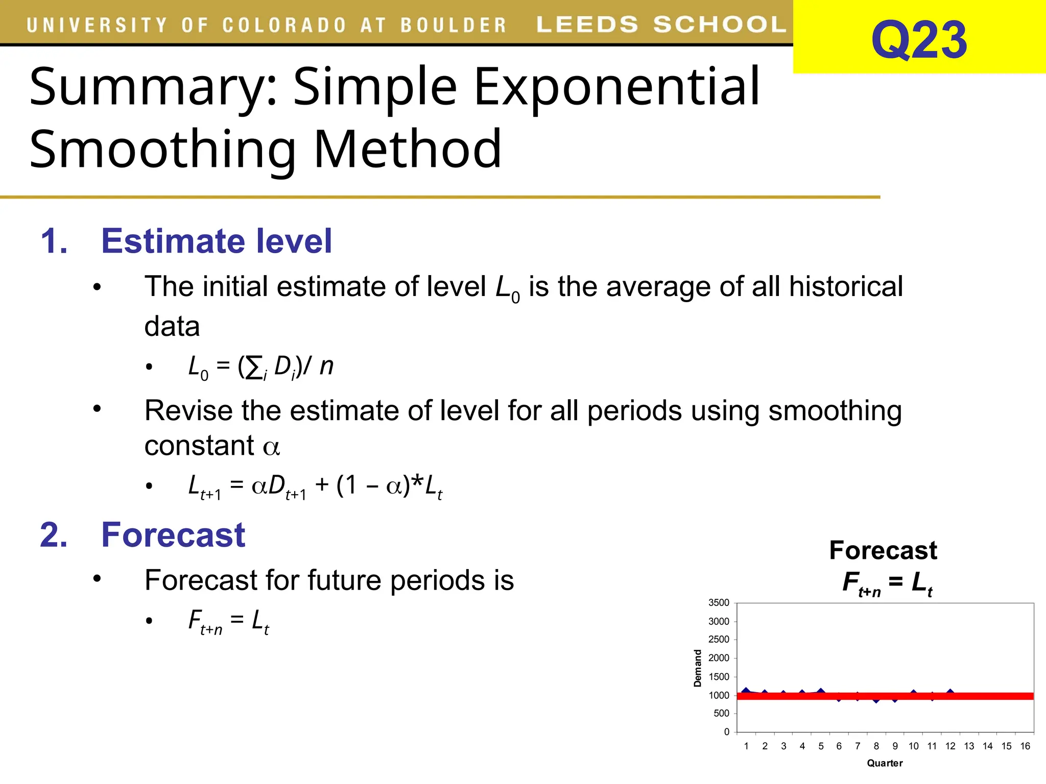
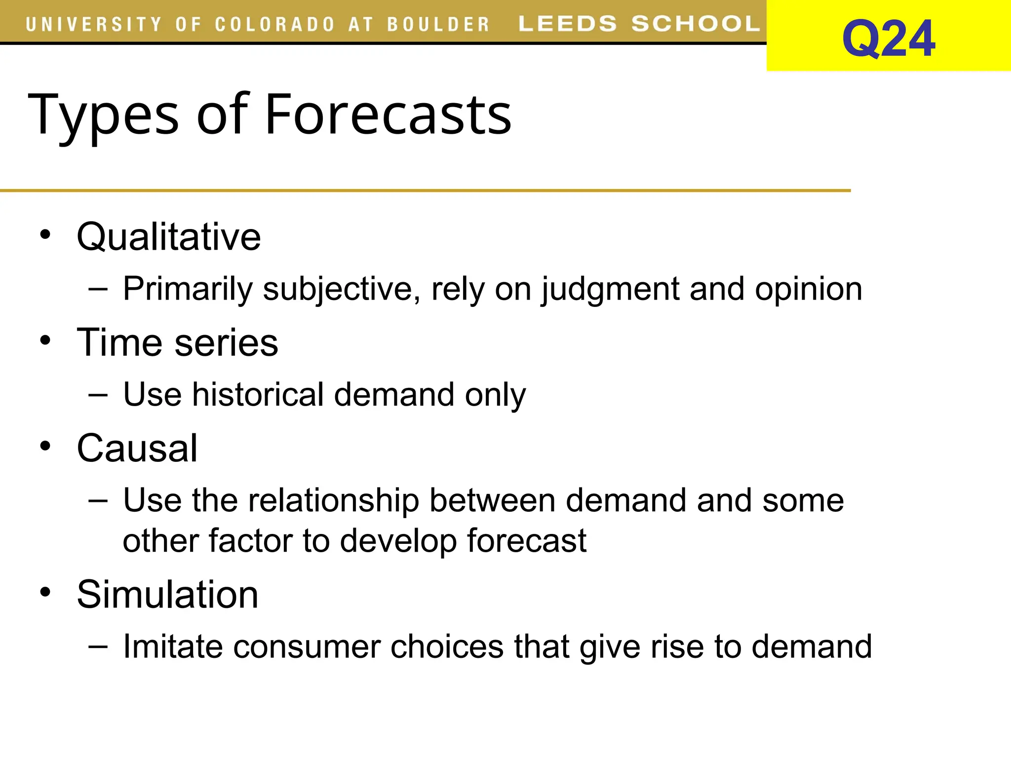
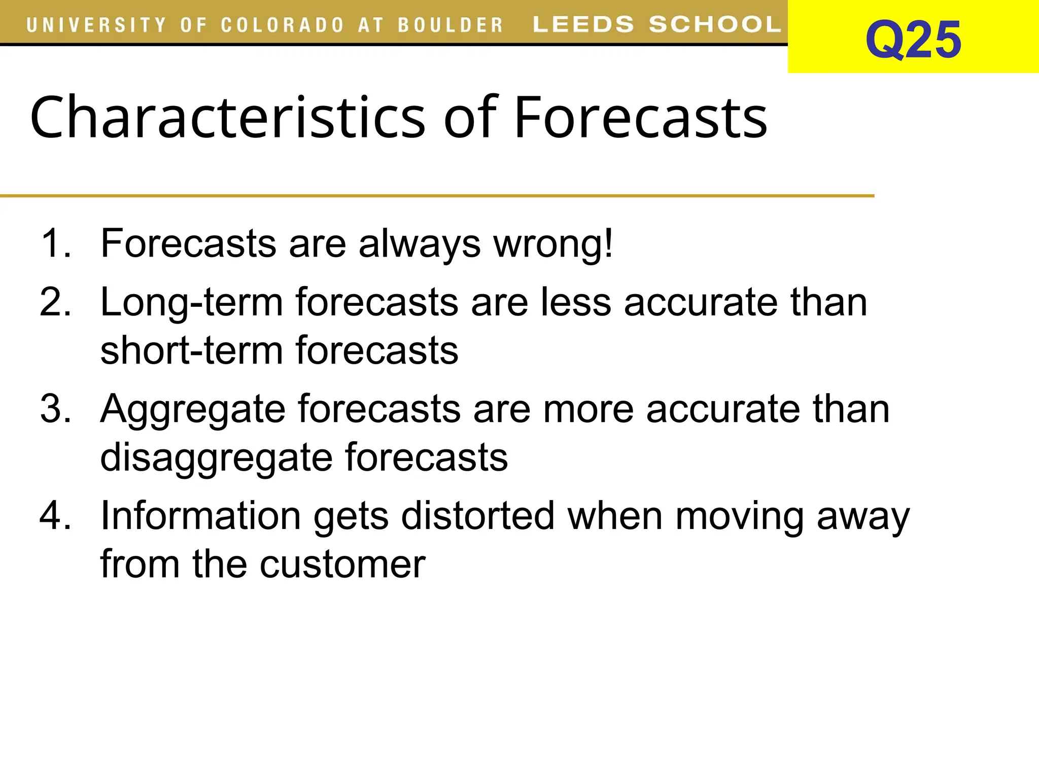
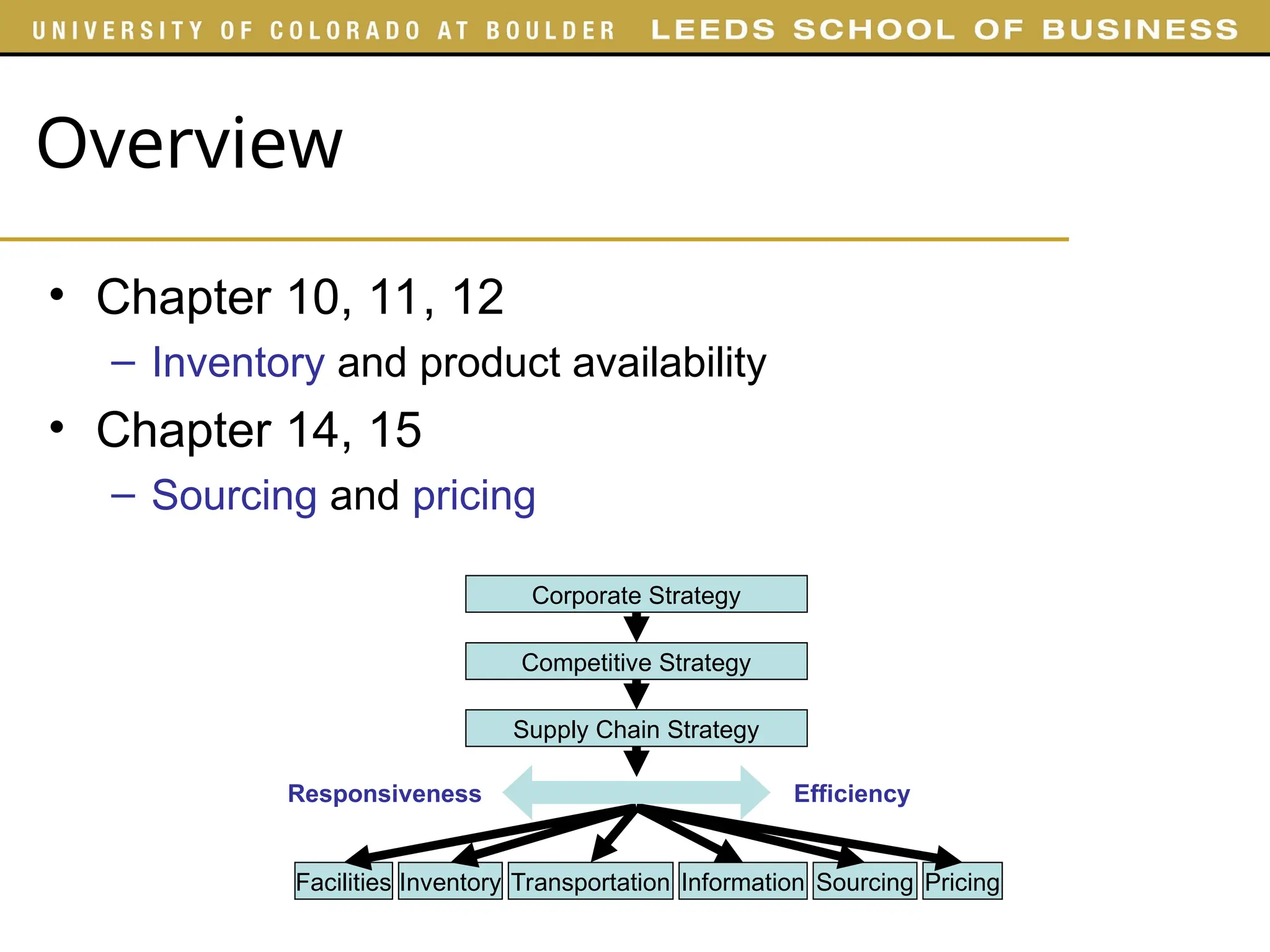
Supply Chain Management
Lecture 17
Outline
• Today
– Survey
– Midterm
– Brief semester overview
– Start with Chapter 10
• Next week
– Chapter 10
• 3e: Sections 1, 2 (up to page 273), 6
• 4e: Sections 1, 2, 3 (up to page 260)
Supply Chain Stages
• A typical supply chain may involve a variety of
stages
Manufacturer Distributor Retailer Customer
Supplier
Most supply chains are actually supply networks
Q1
Push/Pull View of Supply Chain
Processes
Customer order arrives
PULL
PROCESSES
PUSH
PROCESSES
Execution is initiated in
response to customer orders
(reactive)
Execution is initiated in
anticipation of customer orders
(speculative)
Processes are divided based on the timing of
their execution relative to a customer order
Q2
Cycle View of Supply Chain Processes
Customer Order Cycle
Replenishment Cycle
Manufacturing Cycle
Procurement Cycle
Customer
Retailer
Distributor
Manufacturer
Supplier
Cycle view
defines the
processes
involved and
the owner of
each process
Q3
2. Understanding the Supply Chain
Capabilities
• Supply chain capabilities
– Supply chain responsiveness
• Respond to wide ranges of quantity demanded, meet short
lead times, large variety, innovative products, high service
level, etc
– Supply chain efficiency (low cost)
Highly
efficient
Highly
responsive
Somewhat
responsive
Somewhat
efficient
Integrated steel
mills
Hanes apparel Most automotive
production
Seven-Eleven
Japan
Q4
1. Understanding the Customer and
Supply Chain Uncertainty
• Understanding customer uncertainty
– Demand varies along certain attributes
• Quantity in each lot, response time, variety of products needed,
convenience, price, innovation, etc
– Implied demand uncertainty
• Demand uncertainty due to the portion of demand that the supply
chain is targeting, not the entire demand
Customer need Causes implied demand uncertainty to…
Range of quantity increases
Response time decreases
Variety of products increases
Number of channels through which
product may be aquired increases
Rate of innovation increases
Required service level increases
Customer need Causes implied demand uncertainty to…
Range of quantity increases Increase
Response time decreases Increase
Variety of products increases Increase
Number of channels through which
product may be aquired increases
Increase
Rate of innovation increases Increase
Required service level increases Increase
Q5
Key Observations
1. There is no supply chain strategy that is always
right
2. There is a right supply chain strategy for a given
competitive strategy
Q6
From Strategy to Decisions
Corporate Strategy
Competitive Strategy
Supply Chain Strategy
Responsiveness Efficiency
Facilities Inventory Transportation Information Sourcing Pricing
Logistical drivers Cross functional drivers
Q7
2. Understanding the Supply Chain
Capabilities
• Supply chain capabilities
– Supply chain responsiveness
• Respond to wide ranges of quantity demanded, meet short
lead times, large variety, innovative products, high service
level, etc
– Supply chain efficiency (low cost)
Highly
efficient
Highly
responsive
Somewhat
responsive
Somewhat
efficient
Integrated steel
mills
Hanes apparel Most automotive
production
Seven-Eleven
Japan
Q8
Transportation Cost and Number of
Facilities
Number of
Facilities
Transportation
Costs
Q9
Response Time and Number of
Facilities
Number of
Facilities
Response
Time
Q10
Factors Influencing Distribution
Network Design
• Performance of a distribution network should be evaluated
along two dimensions
– Customer needs that are met (customer service)
• Response time (Time it takes for a customer to receive an order)
• Product variety (Number of different products that are offered)
• Product availability (Probability of having a product in stock)
• Customer experience (Ease of placing and receiving orders)
• Order visibility (Ability of customers to track their orders)
• Returnability (Ease of returning unsatisfactory merchandise)
– Cost of meeting customer needs (supply chain cost)
• Inventory (All raw materials, WIP, and finished goods)
• Transportation (Moving inventory from point to point)
• Facility & handling (Locations where product is stored, assembled, or
fabricated)
• Information (Data and analysis of all drivers in a supply chain)
Q11
Retail Storage with Customer Pickup
• Example: Retail stores such as
Wal-Mart and JCPenney
• Customers pick up product from
retailers
– Low transportation cost
– High facility cost
– Relative easy returnability
– Increased inventory cost
• No order tracking necessary
– If the product is available at the
retailer, the consumer buys.
Otherwise goes to another
retailer
• Effective for fast moving items
Retailer
Consumers
Retailer
Retailer
Distributor
Warehouse
Manufacturers
Distributor
Warehouse
Q12
Distributor Storage with Carrier
Delivery
• Example: Amazon
• Inventory is held at a
warehouse which ships to
customer by carriers
• With respect to direct shipping
– Inventory aggregation is less
– Higher inventory costs
– Facility costs are higher
– Less information to track
• Warehouses are physically
closer to consumers which
leads to
– Faster response time
– Lower transportation cost
• Not effective for slow moving
items
Distributor
Warehouse
Manufacturers
Consumers
Distributor
Warehouse
Q13
Manufacturer Storage with Direct
Shipping (Drop Shipping)
• Example: eBags
• Products are shipped directly to
the consumer from the
manufacturer
• Retailer is an information
collector:
– Passes orders to the
manufacturers
– It does not hold product
inventory
• Inventory is centralized at
manufacturer
• Drop shipping offers the
manufacturer the opportunity to
postpone customization
• Effective for high value, large
variety, low demand products
• High transportation cost
Retailer
Manufacturers
Consumers
Q14
Inventory Cost and Number of
Facilities
Number of
Facilities
Inventory
Costs
Q15
Total Logistics Costs
Inventory Costs
Logistics
Costs
Number of
Facilities
Transportation Costs
Facility Costs
Logistics Costs
Q16
Factors Influencing Network Design
Decisions
• Technological factors
– Compare your supplies to the final product, considering whether
value, weight, volume or other factors change
– Availability of production technologies
– High or low fixed cost
• Semiconductor manufacturing takes place only in 5-6 countries
worldwide (building one plant costs about 1 to 4 billion dollars)
Which products gain/lose weight in the
production process?
Q17
Factors Influencing Network Design
Decisions
• Political factors
– Political stability
• Infrastructure factors
– Availability of transportation terminals, labor
• Most of Amazon’s distribution centers are located near airports
• Competitive factors
– Positive externalities (many stores in a mall makes it more
convenient for customers – one location for everything the
customers need)
Q18
Factors Influencing Network Design
Decisions
• Technological factors
– Compare your supplies to the final product, considering whether
value, weight, volume or other factors change
– Availability of production technologies
– High or low fixed cost
• Semiconductor manufacturing takes place only in 5-6 countries
worldwide (building one plant costs about 1 to 4 billion dollars)
Which products gain/lose weight in the
production process?
Q19
Discounted Cash Flow Analysis
• The present value of future cash is found by
using a rate of return k
– A dollar today is worth more than a dollar tomorrow
– A dollar today can be invested and earn a rate of return
k over the next period
Today… Tomorrow…
$1 $1*(1 + k)
$1/(1 + k) $1
Today… Tomorrow…
$1 $1*(1 + k)
Q20
Impact of Uncertainty in Network
Design
Manufacturer Distributor Retailer Customer
Supplier
Building flexibility into supply chain operations allows
the supply chain to deal with uncertainty more
effectively
Q21
Role of Forecasting
Push Push Push
Push Push
Push
Pull
Pull
Pull
Manufacturer Distributor Retailer Customer
Supplier
Is demand forecasting more important
for a push or pull system?
Q22
Summary: Simple Exponential
Smoothing Method
1. Estimate level
• The initial estimate of level L0 is the average of all historical
data
• L0 = (∑i Di)/ n
• Revise the estimate of level for all periods using smoothing
constant 
• Lt+1 = Dt+1 + (1 – )*Lt
2. Forecast
• Forecast for future periods is
• Ft+n = Lt
0
500
1000
1500
2000
2500
3000
3500
1 2 3 4 5 6 7 8 9 10 11 12 13 14 15 16
Quarter
Demand
Forecast
Ft+n = Lt
Q23
Types of Forecasts
• Qualitative
– Primarily subjective, rely on judgment and opinion
• Time series
– Use historical demand only
• Causal
– Use the relationship between demand and some
other factor to develop forecast
• Simulation
– Imitate consumer choices that give rise to demand
Q24
Characteristics of Forecasts
1. Forecasts are always wrong!
2. Long-term forecasts are less accurate than
short-term forecasts
3. Aggregate forecasts are more accurate than
disaggregate forecasts
4. Information gets distorted when moving away
from the customer
Q25
Time Series Forecasting
Observed demand =
Systematic component + Random component
L Level (current deseasonalized demand)
T Trend (growth or decline in demand)
S Seasonality (predictable seasonal fluctuation)
The goal of any forecasting method is to predict the systematic
component (Forecast) of demand and measure the size and
variability of the random component (Forecast error)
Q26
Aggregate Planning Strategies
• Basic strategies
– Level strategy (using inventory as lever)
• Synchronize production rate with long term average demand
• Swim wear
– Chase (the demand) strategy (using capacity as lever)
• Synchronize production rate with demand
• Fast food restaurants
– Time flexibility strategy (using utilization as lever)
• High levels excess (machine and/or workforce) capacity
• Machine shops, army
– Tailored strategy
• Combination of the chase, level, and time flexibility strategies
Q27
Q28
Period Demand Level
0
1 356
2 270
3 257
4 292
5 352
6 293
F6 = L5
L5 = (D5+D4+D3+D2)/4
L5 = 292.75
Period Demand Level Trend
0 104.0 3.5
1 108 107.6 3.5
2 110 110.9 3.5
3 115 114.5 3.5
0
500
1000
1500
2000
2500
3000
3500
1 2 3 4 5 6 7 8 9 10 11 12 13 14 15 16
Quarter
Demand
Forecast
Ft+n = Lt + nTt
F6 = L3 + 3T3
F5 = 125.0
Q29
Period Demand Forecast Mean
Absolute
% Error
0
1 190 211
2 235 225
APE1 = |E1/D1|*100 = 11.05
APE2 = |E2/D2|*100 = 4.26
MAPE2 = (APE1 + APE2)/2 = 7.65
Q30
Overview
• Chapter 10, 11, 12
– Inventory and product availability
• Chapter 14, 15
– Sourcing and pricing
Corporate Strategy
Competitive Strategy
Supply Chain Strategy
Responsiveness Efficiency
Facilities Inventory Transportation Information Sourcing Pricing
Types of Inventory
• Raw material inventory
– Stocked at plant or supplier
– Lowest cost
• Work-in-process (WIP) Inventory
– Raw materials transformed by operations
– Need just enough
• Finished-goods inventory
– WIP after final operation
– Stocked at plant, DC, retail store
High
flexibility
High
cost
The Importance of Inventory
Every other time in the modern era that the U.S. economy has
contracted more than 5% in a quarter, falling inventories have been a
major reason, if not the single biggest factor. Usually, really bad
recessions are worsened by the need for companies to get rid of all the
stuff they made but nobody bought. Once the inventories are sold off,
the economy can grow quickly again because idled workers are called
back.
Source: MarketWatch. Jan 25, 2009
But so far in this recession, the inventory cycle hasn't been a major factor,
outside of the housing and auto sectors. … This recession is rooted in a
severe credit squeeze and a fundamental readjustment in consumer
demand, not in the typical inventory cycle.
The Importance of Inventory
• Firms can reduce costs by reducing inventory, but
customers become dissatisfied when an item is
out of stock
The objective of inventory management is to
strike a balance between inventory investment
and customer service
Demand
• Average demand for Jacob’s product in Pangea
– Existing and new markets
0
20
40
60
80
100
120
1 145 289 433 577 721 865 1009 1153 1297 1441
0
20
40
60
80
100
120
140
1 145 289 433 577 721 865 1009 1153 1297 1441
0
2
4
6
8
10
12
14
16
18
1 142 283 424 565 706 847 988 1129 1270 1411
0
2
4
6
8
10
12
14
16
18
1 142 283 424 565 706 847 988 1129 1270 1411
0
2
4
6
8
10
12
14
16
18
1 142 283 424 565 706 847 988 1129 1270 1411
250
Inventory Decisions
• How much to order?
– Order quantity or lot size (Q)
• When to order?
– Order frequency (n)
Find an inventory policy that is optimal with
respect to some criteria (usually cost)
Inventory Profile
Inventory
Time
Q
Q/2
0
Cycle
Lot
size
Q
Average demand D
Average
inventory
due
to
cycle
inventory
Q/2
Average inventory
Average demand
Average flow time = = Q/2D
Cycle Inventory: Example
• Given
– Q = 1000 units (lot size)
– D = 100 units/day (demand)
• Average inventory
– Q/2 = 1000/2 = 500 (average inventory level from cycle inventory)
• Average flow time
– Q/2D = 1000/(2*100) = 5 days (time a unit spends in the supply chain)
• Lower inventory is better because
– Average flow time is lower
– Working capital requirements are lower
– Lower inventory holding costs
Why Order in Large/Small Lots?
• Fixed ordering cost: S (cost incurred per order)
– Increase the lot size to decrease the fixed ordering cost per unit
• Holding cost: H (cost of carrying one unit in inventory)
– Decrease the lot size to decrease holding cost
• Material cost: C (cost per unit)
Lot size Q is chosen by trading off holding
costs against fixed ordering costs
Fixed cost Material cost
Convenience store Low High
Sam's Club High Low
Economies of Scale to Exploit Fixed
Costs
• Economic order quantity (EOQ)
– Optimal lot size for a single product

PushPull View of Supply Chain Processes.ppt

  • 1.
  • 2.
    Outline • Today – Survey –Midterm – Brief semester overview – Start with Chapter 10 • Next week – Chapter 10 • 3e: Sections 1, 2 (up to page 273), 6 • 4e: Sections 1, 2, 3 (up to page 260)
  • 3.
    Supply Chain Stages •A typical supply chain may involve a variety of stages Manufacturer Distributor Retailer Customer Supplier Most supply chains are actually supply networks Q1
  • 4.
    Push/Pull View ofSupply Chain Processes Customer order arrives PULL PROCESSES PUSH PROCESSES Execution is initiated in response to customer orders (reactive) Execution is initiated in anticipation of customer orders (speculative) Processes are divided based on the timing of their execution relative to a customer order Q2
  • 5.
    Cycle View ofSupply Chain Processes Customer Order Cycle Replenishment Cycle Manufacturing Cycle Procurement Cycle Customer Retailer Distributor Manufacturer Supplier Cycle view defines the processes involved and the owner of each process Q3
  • 6.
    2. Understanding theSupply Chain Capabilities • Supply chain capabilities – Supply chain responsiveness • Respond to wide ranges of quantity demanded, meet short lead times, large variety, innovative products, high service level, etc – Supply chain efficiency (low cost) Highly efficient Highly responsive Somewhat responsive Somewhat efficient Integrated steel mills Hanes apparel Most automotive production Seven-Eleven Japan Q4
  • 7.
    1. Understanding theCustomer and Supply Chain Uncertainty • Understanding customer uncertainty – Demand varies along certain attributes • Quantity in each lot, response time, variety of products needed, convenience, price, innovation, etc – Implied demand uncertainty • Demand uncertainty due to the portion of demand that the supply chain is targeting, not the entire demand Customer need Causes implied demand uncertainty to… Range of quantity increases Response time decreases Variety of products increases Number of channels through which product may be aquired increases Rate of innovation increases Required service level increases Customer need Causes implied demand uncertainty to… Range of quantity increases Increase Response time decreases Increase Variety of products increases Increase Number of channels through which product may be aquired increases Increase Rate of innovation increases Increase Required service level increases Increase Q5
  • 8.
    Key Observations 1. Thereis no supply chain strategy that is always right 2. There is a right supply chain strategy for a given competitive strategy Q6
  • 9.
    From Strategy toDecisions Corporate Strategy Competitive Strategy Supply Chain Strategy Responsiveness Efficiency Facilities Inventory Transportation Information Sourcing Pricing Logistical drivers Cross functional drivers Q7
  • 10.
    2. Understanding theSupply Chain Capabilities • Supply chain capabilities – Supply chain responsiveness • Respond to wide ranges of quantity demanded, meet short lead times, large variety, innovative products, high service level, etc – Supply chain efficiency (low cost) Highly efficient Highly responsive Somewhat responsive Somewhat efficient Integrated steel mills Hanes apparel Most automotive production Seven-Eleven Japan Q8
  • 11.
    Transportation Cost andNumber of Facilities Number of Facilities Transportation Costs Q9
  • 12.
    Response Time andNumber of Facilities Number of Facilities Response Time Q10
  • 13.
    Factors Influencing Distribution NetworkDesign • Performance of a distribution network should be evaluated along two dimensions – Customer needs that are met (customer service) • Response time (Time it takes for a customer to receive an order) • Product variety (Number of different products that are offered) • Product availability (Probability of having a product in stock) • Customer experience (Ease of placing and receiving orders) • Order visibility (Ability of customers to track their orders) • Returnability (Ease of returning unsatisfactory merchandise) – Cost of meeting customer needs (supply chain cost) • Inventory (All raw materials, WIP, and finished goods) • Transportation (Moving inventory from point to point) • Facility & handling (Locations where product is stored, assembled, or fabricated) • Information (Data and analysis of all drivers in a supply chain) Q11
  • 14.
    Retail Storage withCustomer Pickup • Example: Retail stores such as Wal-Mart and JCPenney • Customers pick up product from retailers – Low transportation cost – High facility cost – Relative easy returnability – Increased inventory cost • No order tracking necessary – If the product is available at the retailer, the consumer buys. Otherwise goes to another retailer • Effective for fast moving items Retailer Consumers Retailer Retailer Distributor Warehouse Manufacturers Distributor Warehouse Q12
  • 15.
    Distributor Storage withCarrier Delivery • Example: Amazon • Inventory is held at a warehouse which ships to customer by carriers • With respect to direct shipping – Inventory aggregation is less – Higher inventory costs – Facility costs are higher – Less information to track • Warehouses are physically closer to consumers which leads to – Faster response time – Lower transportation cost • Not effective for slow moving items Distributor Warehouse Manufacturers Consumers Distributor Warehouse Q13
  • 16.
    Manufacturer Storage withDirect Shipping (Drop Shipping) • Example: eBags • Products are shipped directly to the consumer from the manufacturer • Retailer is an information collector: – Passes orders to the manufacturers – It does not hold product inventory • Inventory is centralized at manufacturer • Drop shipping offers the manufacturer the opportunity to postpone customization • Effective for high value, large variety, low demand products • High transportation cost Retailer Manufacturers Consumers Q14
  • 17.
    Inventory Cost andNumber of Facilities Number of Facilities Inventory Costs Q15
  • 18.
    Total Logistics Costs InventoryCosts Logistics Costs Number of Facilities Transportation Costs Facility Costs Logistics Costs Q16
  • 19.
    Factors Influencing NetworkDesign Decisions • Technological factors – Compare your supplies to the final product, considering whether value, weight, volume or other factors change – Availability of production technologies – High or low fixed cost • Semiconductor manufacturing takes place only in 5-6 countries worldwide (building one plant costs about 1 to 4 billion dollars) Which products gain/lose weight in the production process? Q17
  • 20.
    Factors Influencing NetworkDesign Decisions • Political factors – Political stability • Infrastructure factors – Availability of transportation terminals, labor • Most of Amazon’s distribution centers are located near airports • Competitive factors – Positive externalities (many stores in a mall makes it more convenient for customers – one location for everything the customers need) Q18
  • 21.
    Factors Influencing NetworkDesign Decisions • Technological factors – Compare your supplies to the final product, considering whether value, weight, volume or other factors change – Availability of production technologies – High or low fixed cost • Semiconductor manufacturing takes place only in 5-6 countries worldwide (building one plant costs about 1 to 4 billion dollars) Which products gain/lose weight in the production process? Q19
  • 22.
    Discounted Cash FlowAnalysis • The present value of future cash is found by using a rate of return k – A dollar today is worth more than a dollar tomorrow – A dollar today can be invested and earn a rate of return k over the next period Today… Tomorrow… $1 $1*(1 + k) $1/(1 + k) $1 Today… Tomorrow… $1 $1*(1 + k) Q20
  • 23.
    Impact of Uncertaintyin Network Design Manufacturer Distributor Retailer Customer Supplier Building flexibility into supply chain operations allows the supply chain to deal with uncertainty more effectively Q21
  • 24.
    Role of Forecasting PushPush Push Push Push Push Pull Pull Pull Manufacturer Distributor Retailer Customer Supplier Is demand forecasting more important for a push or pull system? Q22
  • 25.
    Summary: Simple Exponential SmoothingMethod 1. Estimate level • The initial estimate of level L0 is the average of all historical data • L0 = (∑i Di)/ n • Revise the estimate of level for all periods using smoothing constant  • Lt+1 = Dt+1 + (1 – )*Lt 2. Forecast • Forecast for future periods is • Ft+n = Lt 0 500 1000 1500 2000 2500 3000 3500 1 2 3 4 5 6 7 8 9 10 11 12 13 14 15 16 Quarter Demand Forecast Ft+n = Lt Q23
  • 26.
    Types of Forecasts •Qualitative – Primarily subjective, rely on judgment and opinion • Time series – Use historical demand only • Causal – Use the relationship between demand and some other factor to develop forecast • Simulation – Imitate consumer choices that give rise to demand Q24
  • 27.
    Characteristics of Forecasts 1.Forecasts are always wrong! 2. Long-term forecasts are less accurate than short-term forecasts 3. Aggregate forecasts are more accurate than disaggregate forecasts 4. Information gets distorted when moving away from the customer Q25
  • 28.
    Time Series Forecasting Observeddemand = Systematic component + Random component L Level (current deseasonalized demand) T Trend (growth or decline in demand) S Seasonality (predictable seasonal fluctuation) The goal of any forecasting method is to predict the systematic component (Forecast) of demand and measure the size and variability of the random component (Forecast error) Q26
  • 29.
    Aggregate Planning Strategies •Basic strategies – Level strategy (using inventory as lever) • Synchronize production rate with long term average demand • Swim wear – Chase (the demand) strategy (using capacity as lever) • Synchronize production rate with demand • Fast food restaurants – Time flexibility strategy (using utilization as lever) • High levels excess (machine and/or workforce) capacity • Machine shops, army – Tailored strategy • Combination of the chase, level, and time flexibility strategies Q27
  • 30.
    Q28 Period Demand Level 0 1356 2 270 3 257 4 292 5 352 6 293 F6 = L5 L5 = (D5+D4+D3+D2)/4 L5 = 292.75
  • 31.
    Period Demand LevelTrend 0 104.0 3.5 1 108 107.6 3.5 2 110 110.9 3.5 3 115 114.5 3.5 0 500 1000 1500 2000 2500 3000 3500 1 2 3 4 5 6 7 8 9 10 11 12 13 14 15 16 Quarter Demand Forecast Ft+n = Lt + nTt F6 = L3 + 3T3 F5 = 125.0 Q29
  • 32.
    Period Demand ForecastMean Absolute % Error 0 1 190 211 2 235 225 APE1 = |E1/D1|*100 = 11.05 APE2 = |E2/D2|*100 = 4.26 MAPE2 = (APE1 + APE2)/2 = 7.65 Q30
  • 33.
    Overview • Chapter 10,11, 12 – Inventory and product availability • Chapter 14, 15 – Sourcing and pricing Corporate Strategy Competitive Strategy Supply Chain Strategy Responsiveness Efficiency Facilities Inventory Transportation Information Sourcing Pricing
  • 34.
    Types of Inventory •Raw material inventory – Stocked at plant or supplier – Lowest cost • Work-in-process (WIP) Inventory – Raw materials transformed by operations – Need just enough • Finished-goods inventory – WIP after final operation – Stocked at plant, DC, retail store High flexibility High cost
  • 35.
    The Importance ofInventory Every other time in the modern era that the U.S. economy has contracted more than 5% in a quarter, falling inventories have been a major reason, if not the single biggest factor. Usually, really bad recessions are worsened by the need for companies to get rid of all the stuff they made but nobody bought. Once the inventories are sold off, the economy can grow quickly again because idled workers are called back. Source: MarketWatch. Jan 25, 2009 But so far in this recession, the inventory cycle hasn't been a major factor, outside of the housing and auto sectors. … This recession is rooted in a severe credit squeeze and a fundamental readjustment in consumer demand, not in the typical inventory cycle.
  • 36.
    The Importance ofInventory • Firms can reduce costs by reducing inventory, but customers become dissatisfied when an item is out of stock The objective of inventory management is to strike a balance between inventory investment and customer service
  • 37.
    Demand • Average demandfor Jacob’s product in Pangea – Existing and new markets 0 20 40 60 80 100 120 1 145 289 433 577 721 865 1009 1153 1297 1441 0 20 40 60 80 100 120 140 1 145 289 433 577 721 865 1009 1153 1297 1441 0 2 4 6 8 10 12 14 16 18 1 142 283 424 565 706 847 988 1129 1270 1411 0 2 4 6 8 10 12 14 16 18 1 142 283 424 565 706 847 988 1129 1270 1411 0 2 4 6 8 10 12 14 16 18 1 142 283 424 565 706 847 988 1129 1270 1411 250
  • 38.
    Inventory Decisions • Howmuch to order? – Order quantity or lot size (Q) • When to order? – Order frequency (n) Find an inventory policy that is optimal with respect to some criteria (usually cost)
  • 39.
    Inventory Profile Inventory Time Q Q/2 0 Cycle Lot size Q Average demandD Average inventory due to cycle inventory Q/2 Average inventory Average demand Average flow time = = Q/2D
  • 40.
    Cycle Inventory: Example •Given – Q = 1000 units (lot size) – D = 100 units/day (demand) • Average inventory – Q/2 = 1000/2 = 500 (average inventory level from cycle inventory) • Average flow time – Q/2D = 1000/(2*100) = 5 days (time a unit spends in the supply chain) • Lower inventory is better because – Average flow time is lower – Working capital requirements are lower – Lower inventory holding costs
  • 41.
    Why Order inLarge/Small Lots? • Fixed ordering cost: S (cost incurred per order) – Increase the lot size to decrease the fixed ordering cost per unit • Holding cost: H (cost of carrying one unit in inventory) – Decrease the lot size to decrease holding cost • Material cost: C (cost per unit) Lot size Q is chosen by trading off holding costs against fixed ordering costs Fixed cost Material cost Convenience store Low High Sam's Club High Low
  • 42.
    Economies of Scaleto Exploit Fixed Costs • Economic order quantity (EOQ) – Optimal lot size for a single product

Editor's Notes

  • #4 Processes are divided based on their timing relative to the timing of a customer order They key difference is the uncertainty during the two phases At the time of execution of a pull process customer demand is known At the time of execution of a push process customer demand is not known (and must be forecasted)
  • #5 Each cycle occurs at the interface between two successive stages Customer order cycle (customer-retailer) Replenishment cycle (retailer-distributor) Manufacturing cycle (distributor-manufacturer) Procurement cycle (manufacturer-supplier)
  • #6 Celestial Seasoning ProBuild Mortgage Interceptor Body Armor Crocs Netflix
  • #7 Understanding customer uncertainty: Demand varies along certain attributes Implied demand uncertainty is demand uncertainty due to the portion of demand that the supply chain is targeting, not the entire demand Demand uncertainty reflects the uncertainty of customer demand for a product
  • #8 A company’s competitive strategy defines (relative to its competitors) the set of customer needs that it seeks to satisfy through its products and services
  • #9 To understand how a company can improve supply chain performance in terms of responsiveness and efficiency we must examine (and make decisions about) the drivers of supply chain performance
  • #10 Celestial Seasoning ProBuild Mortgage Interceptor Body Armor Crocs Netflix
  • #11 Includes both inbound and outbound transportation cost If the number of facilities is increased to a point where inbound lot sizes are very small and result in a significant loss of economies of scale in inbound transportation, increasing the number of facilities increases total transportation cost
  • #13 Distribution network design options must therefore be compared according to their impact on customer service and the cost to provide this level of service
  • #16 This model is also referred to as drop-shipping. Retailers carries no inventory. All inventory is at the manufacturer’s site. This is eBags model, which takes orders and arranges for the manufacturer’s to ship directly to the customers. Transportation cost is high because the average outbound distance to the end customer is large. Package carriers are used and are more expensive than TL or LTL. A good information infrastructure is needed. Response time tends to be large. eBags Nordstrom.com (for slow moving footwear) W.W. Grainer (for slow moving items)
  • #18 Each company should have at least the number of facilities that minimize total logistics costs
  • #19 Technological factors * High fixed costs (less facilities) – Intel Semiconductor manufacturing * Low fixed costs (more facilities) - Coca Cola bottling Macroeconomic factors * Trade agreements (NAFTA, EU, APTA–Asian Pacific Trade Agreement, AFTZ–African Free Trade Zone) have led to consolidation * End of quotas has led to consolidation of apparel manufacturing in China * Flexible facilities (capacity) can help reduce the effect of exchanges rates Political factors * Infrastructure factors * Amazon distribution centers are all close to airports
  • #21 Technological factors * High fixed costs (less facilities) – Intel Semiconductor manufacturing * Low fixed costs (more facilities) - Coca Cola bottling Macroeconomic factors * Trade agreements (NAFTA, EU, APTA–Asian Pacific Trade Agreement, AFTZ–African Free Trade Zone) have led to consolidation * End of quotas has led to consolidation of apparel manufacturing in China * Flexible facilities (capacity) can help reduce the effect of exchanges rates Political factors * Infrastructure factors * Amazon distribution centers are all close to airports
  • #22 Discount rate: The rate used to discount future cash flows to their present values
  • #23 Natural disasters, supplier bankruptcies, labor disputes, information infrastructure breakdown, inaccurate forecasts, exchange rate risks Uncertainty is propagated through the supply chain(s) and leads to inefficient processes If there is no uncertainty in the supply chain, the performance can be optimal The presence of uncertainty stimulates the creation of buffers in time, capacity and inventory to prevent a possible bad performance of the chain. These buffers restrict the operational performances and may cancel the competitive advantage of the organization
  • #24 Push: in anticipation of customer demand Pull: in response of customer demand Forecasting is used for both push and pull processes Push processes: Managers must plan the level of activity, be it production, transportation, or any other planned activity. Pull processes: Managers must plan the level of available capacity and inventory Always: Managers must forecast what customer demand will be Manufacturer: Production scheduling decisions, materials requirement planning, purchasing Distributor: Ordering, warehouse capacity Retailer: Shelf space Dell orders PC components in anticipation of customer orders (inventory) Dell performs assembly in response to customer orders (capacity) Intel needs forecasts to determine production and inventory levels. Intel’s suppliers need forecasts to determine production and inventory levels. Mature products with stable demand (milk, paper towels) are usually the easiest to forecast. Scheduling existing resources How many employees do we need and when? How much product should we make in anticipation of demand? Acquiring additional resources When are we going to run out of capacity? How many more people will we need? How large will our back-orders be? Determining what resources are needed What kind of machines will we require? Which services are growing in demand? declining? What kind of people should we be hiring?
  • #26 Qualitative They are primarily subjective; rely on judgment and opinion, intuition, surveys, or comparative techniques. They produce information typically no quantitative, and subjective. Its non-scientific nature makes it difficult to standardize or validate for accuracy, Appropriate when there is little historical data or there is market intelligence. Time Series It uses historical demand only; appropriate when the basic demand pattern varies little between years, the basic premise is that the future demand pattern will be mostly a replication. It uses mathematician and statistical models as forecasting tools which can be static or adaptive to new demand patterns. Causal It uses the relationship between demand and some other factor (e.g. the state of the economy, interest rates) to develop forecast. For example, if is know how level service can influence sales, then by knowing the level of service provided, the level of sales can be projected. We can say that service causes sales. Another example is forecasting the impact of price promotion on demand. Usually it is very difficult to find good cause-and-effect relationships. Simulation This method imitates consumer choices that give rise to demand. It can combine time series and causal methods
  • #28 The goal of any forecasting method is to predict the systematic component of demand