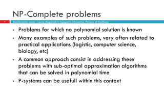
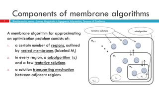
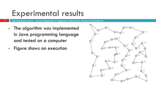
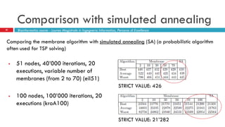
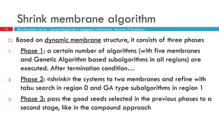
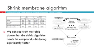
The document discusses the application of membrane algorithms for approximating NP-complete problems, particularly through the example of the Traveling Salesman Problem (TSP). It outlines the structure of membrane algorithms which utilize different subalgorithms to optimize solutions by iterating through regions defined by membranes, along with methods for escaping local minima and parallel implementation. Experimental results indicate that while the membrane algorithm performs comparably to simulated annealing, enhancements through compound and shrink algorithms can significantly improve performance and solution accuracy.


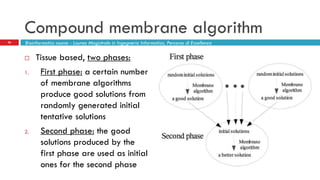
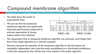


![Getting Started with Apache Spark: Big Data Made Simple [Free Meetup]](https://cdn.slidesharecdn.com/ss_thumbnails/apachesparkgettingstarted-260203175547-8361bcc3-thumbnail.jpg?width=640&height=640&fit=bounds)


