updated UNIT 2.pptxEWDSKJL;MSDCL;MLDSPKDPS

23CSE2018 – Foundations of Artificial Intelligence
Class -S.Y. (SEM-II), AIA
Unit - II PROBLEM SOLVING AND SEARCH
AY 2024-2025 SEM-II
Prof. Sushma Mehetre
MIT School of Computing
Department of Computer Science & Engineering

Unit II: PROBLEM SOLVING AND SEARCH
09 hours
• Problem space and search
• Toy Problems
• Uninformed search methods – Breadth First Search, Uniform Cost Search, Depth First Search,
Depth Limited Search, Iterative Deepening Search, Bi-directional Search
• Heuristic search methods - Best first, Greedy, A* , AO*, Hill Climbing, Local Search and
optimization
• Local Beam Search, Adversarial search -Minimax, Alpha-Beta Pruning
Unit II - Syllabus
Department of Computer Science & Engineering

PROBLEM SOLVING AGENT (GOAL BASED)
⮚What is the Problem?
⮚What can be Solution or Solutions ?
⮚Decide what to do by finding sequences of actions that lead to
desirable states.
⮚General Purpose Search Algorithm to solve problem- analysis of
algorithms
⮚Goal formulation, based on the current situation and the agent's
performance measure, is the first step in problem solving- Tour
Agent Example.
Problem space and search
Department of Computer Science &
Engineering

An agent with several immediate options of unknown value can
decide what to do by just examining different possible sequences of
actions that lead to states of known value, and then choosing the best
sequence.
This process of looking for such a sequence is called Search
Simple steps for achieving goal
Engineering
“Formulate,
Search,
Execute"

Engineering
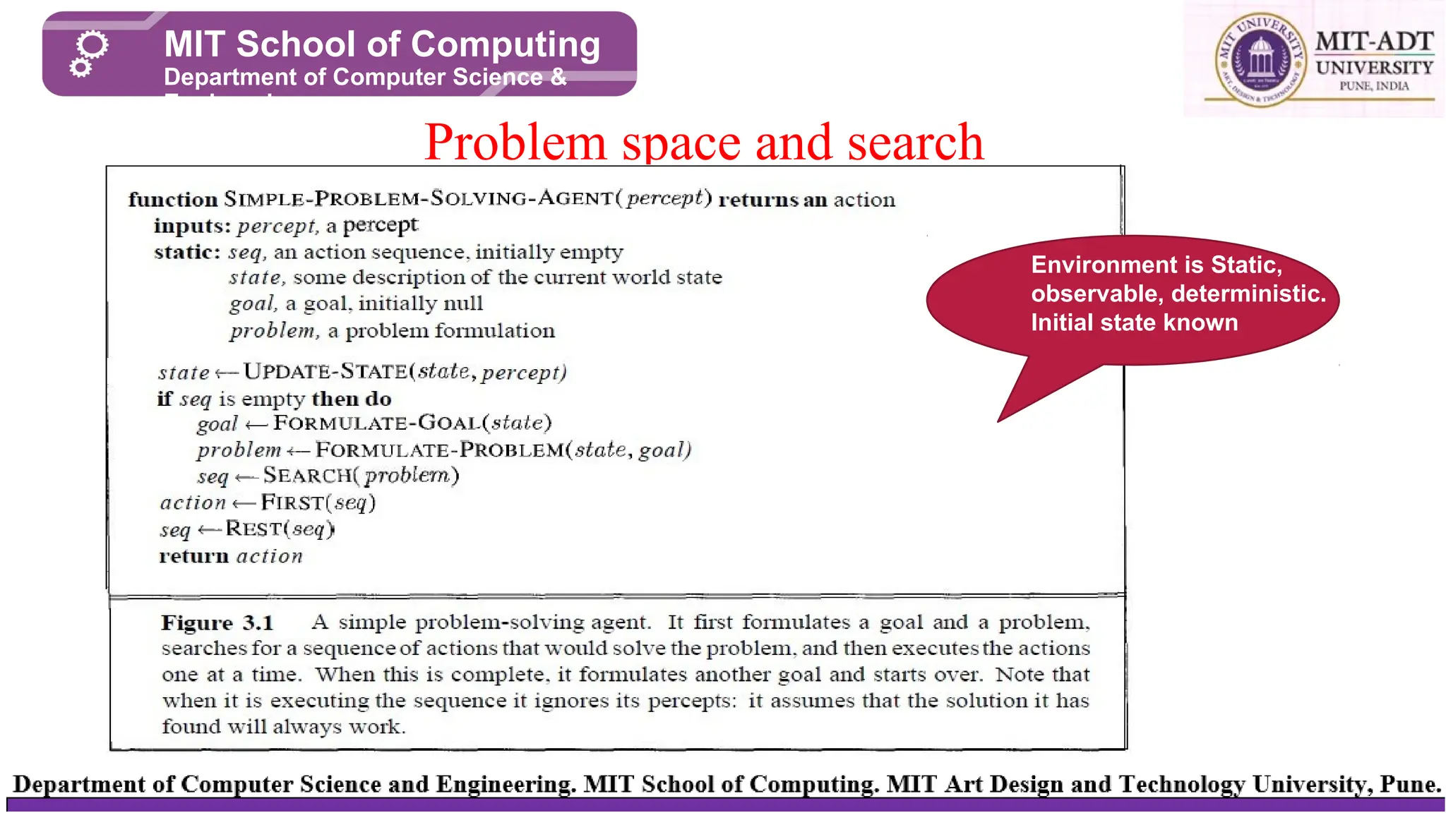
Environment is Static,
observable, deterministic.
Initial state known

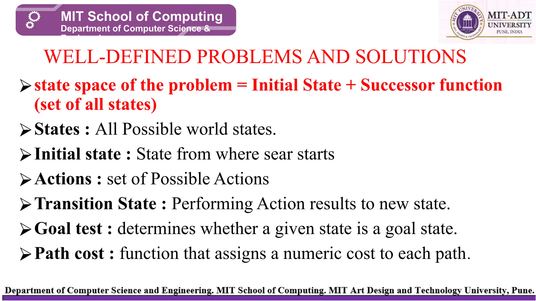
⮚state space of the problem = Initial State + Successor function
(set of all states)
⮚States : All Possible world states.
⮚Initial state : State from where sear starts
⮚Actions : set of Possible Actions
⮚Transition State : Performing Action results to new state.
⮚Goal test : determines whether a given state is a goal state.
⮚Path cost : function that assigns a numeric cost to each path.
WELL-DEFINED PROBLEMS AND SOLUTIONS
Engineering

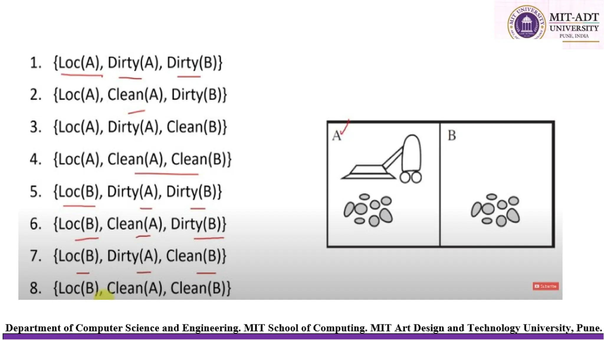
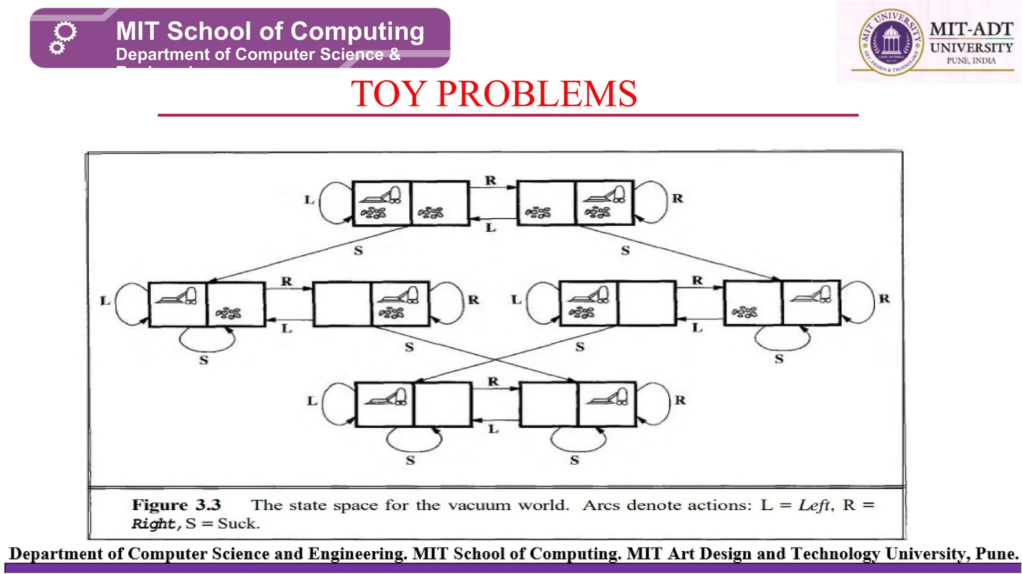
The vacuum world
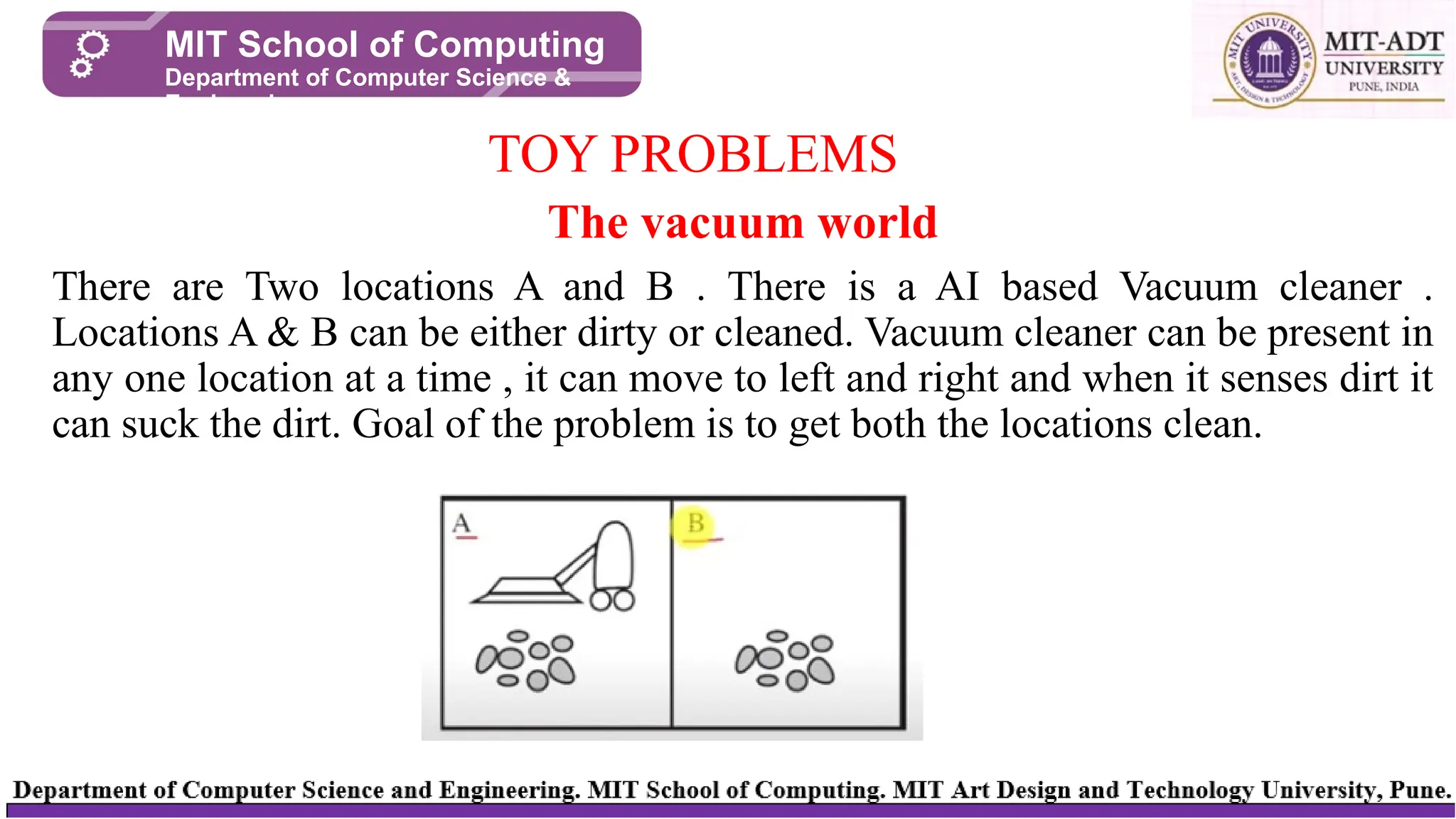
There are Two locations A and B . There is a AI based Vacuum cleaner .
Locations A & B can be either dirty or cleaned. Vacuum cleaner can be present in
any one location at a time , it can move to left and right and when it senses dirt it
can suck the dirt. Goal of the problem is to get both the locations clean.
TOY PROBLEMS
Engineering

TOY PROBLEMS
Engineering

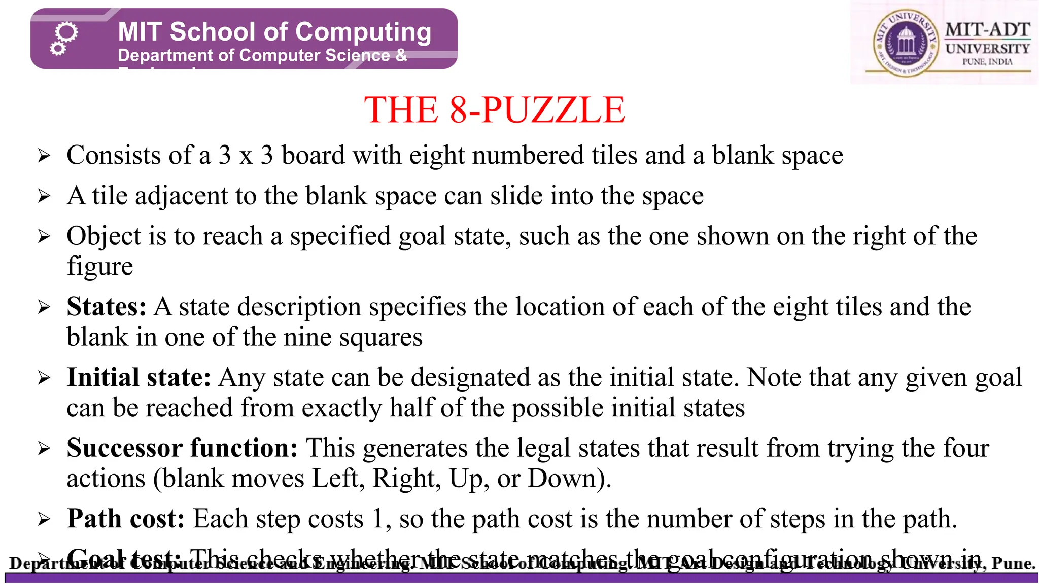
⮚ Consists of a 3 x 3 board with eight numbered tiles and a blank space
⮚ A tile adjacent to the blank space can slide into the space
⮚ Object is to reach a specified goal state, such as the one shown on the right of the
figure
⮚ States: A state description specifies the location of each of the eight tiles and the
blank in one of the nine squares
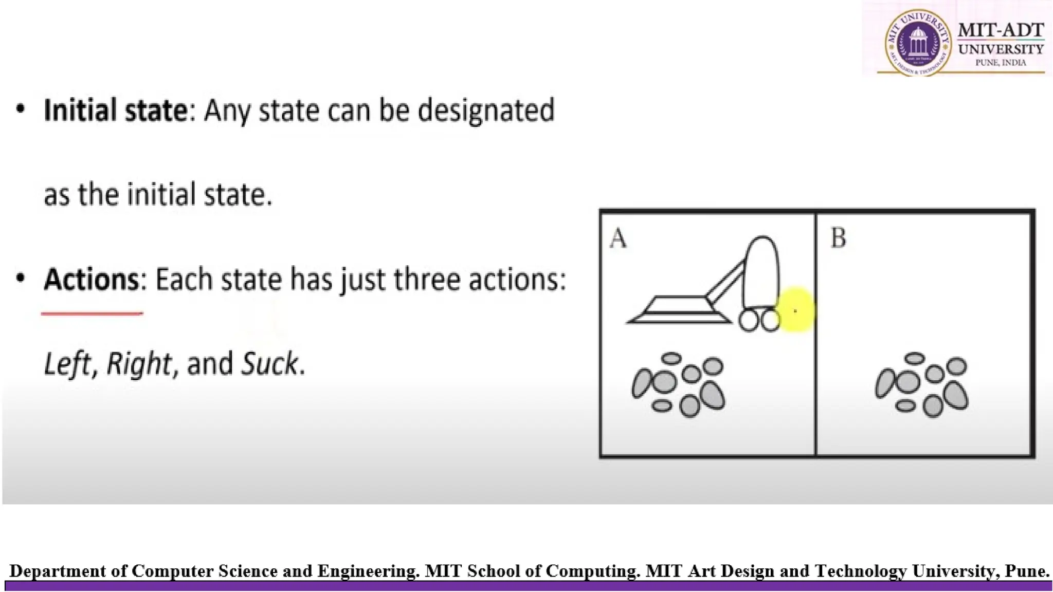
⮚ Initial state: Any state can be designated as the initial state. Note that any given goal
can be reached from exactly half of the possible initial states
⮚ Successor function: This generates the legal states that result from trying the four
actions (blank moves Left, Right, Up, or Down).
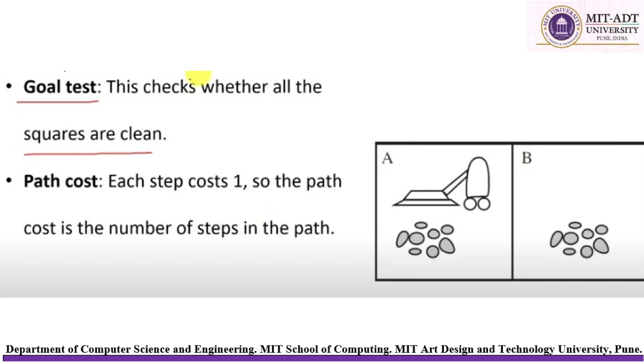
⮚ Path cost: Each step costs 1, so the path cost is the number of steps in the path.
⮚ Goal test: This checks whether the state matches the goal configuration shown in
THE 8-PUZZLE
Engineering

THE 8-PUZZLE
Engineering

THE 8-QUEENS PROBLEM
Engineering
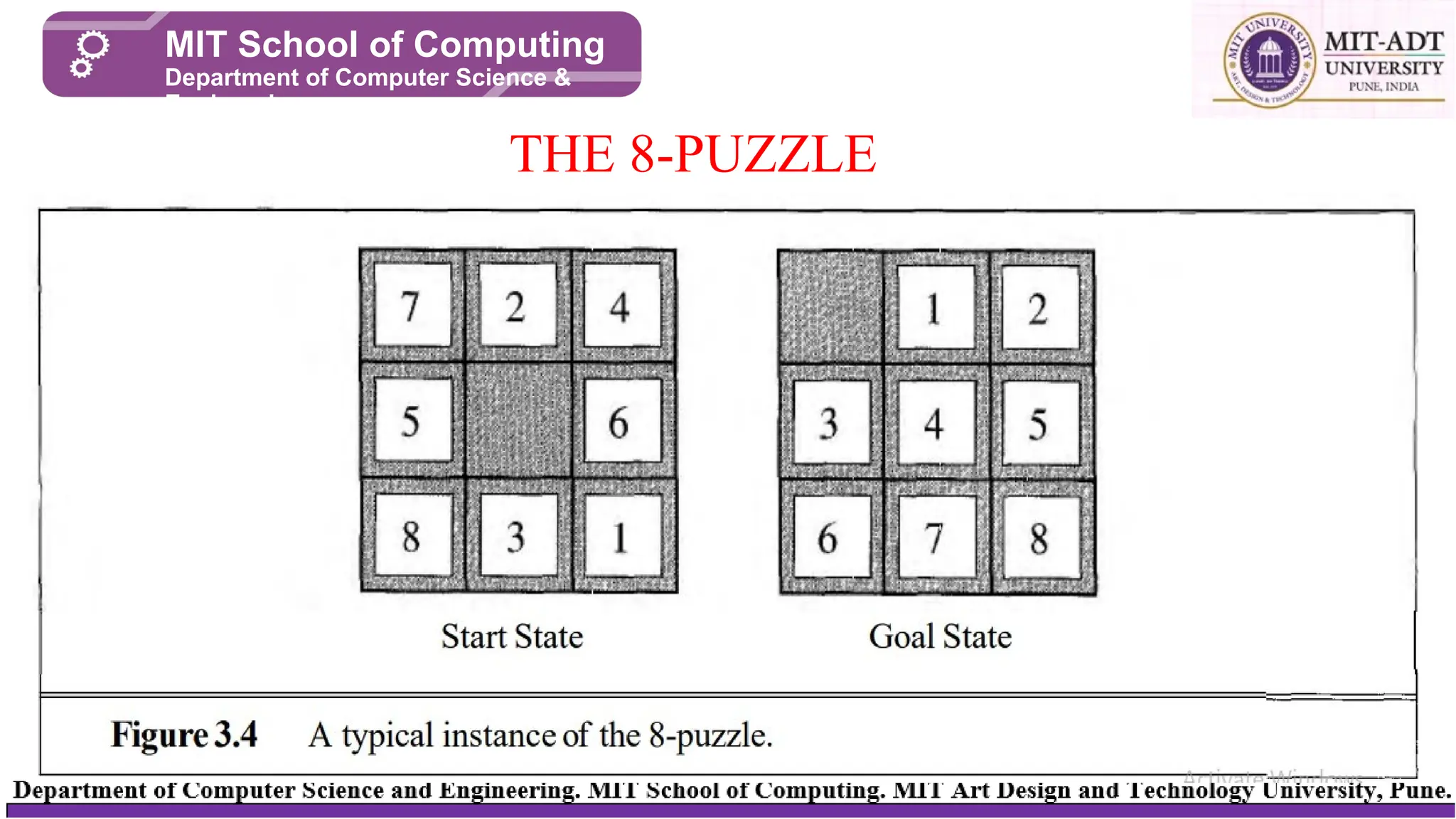
⮚ To place eight queens on a chessboard
such that no queen attacks any other.
⮚ There are two main kinds of formulation.
⮚ An incremental formulation involves
operators that augment the state
description, starting with an empty state;
for the 8-queens problem, this means
that each action adds a queen to the
state.
⮚ A complete-state formulation starts with
all 8 queens on the board and moves
them around. In either case, the path
cost is of no interest because only the
final state counts.

• Search algorithms are fundamental in artificial intelligence (AI) for
problem-solving and pathfinding.
• They are broadly categorized into
• Uninformed (blind) search
• Informed (heuristic) search methods.
Search methods
Engineering

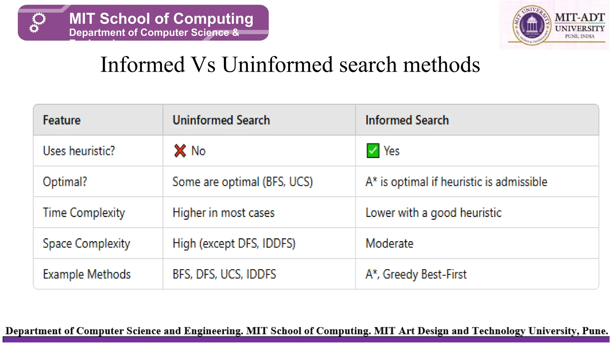
Informed Vs Uninformed search methods
Engineering

• Breadth First Search,
• Uniform Cost Search,
• Depth First Search,
• Depth Limited Search,
• Iterative Deepening Search,
• Bi-directional Search
Uninformed search methods
Engineering

Engineering
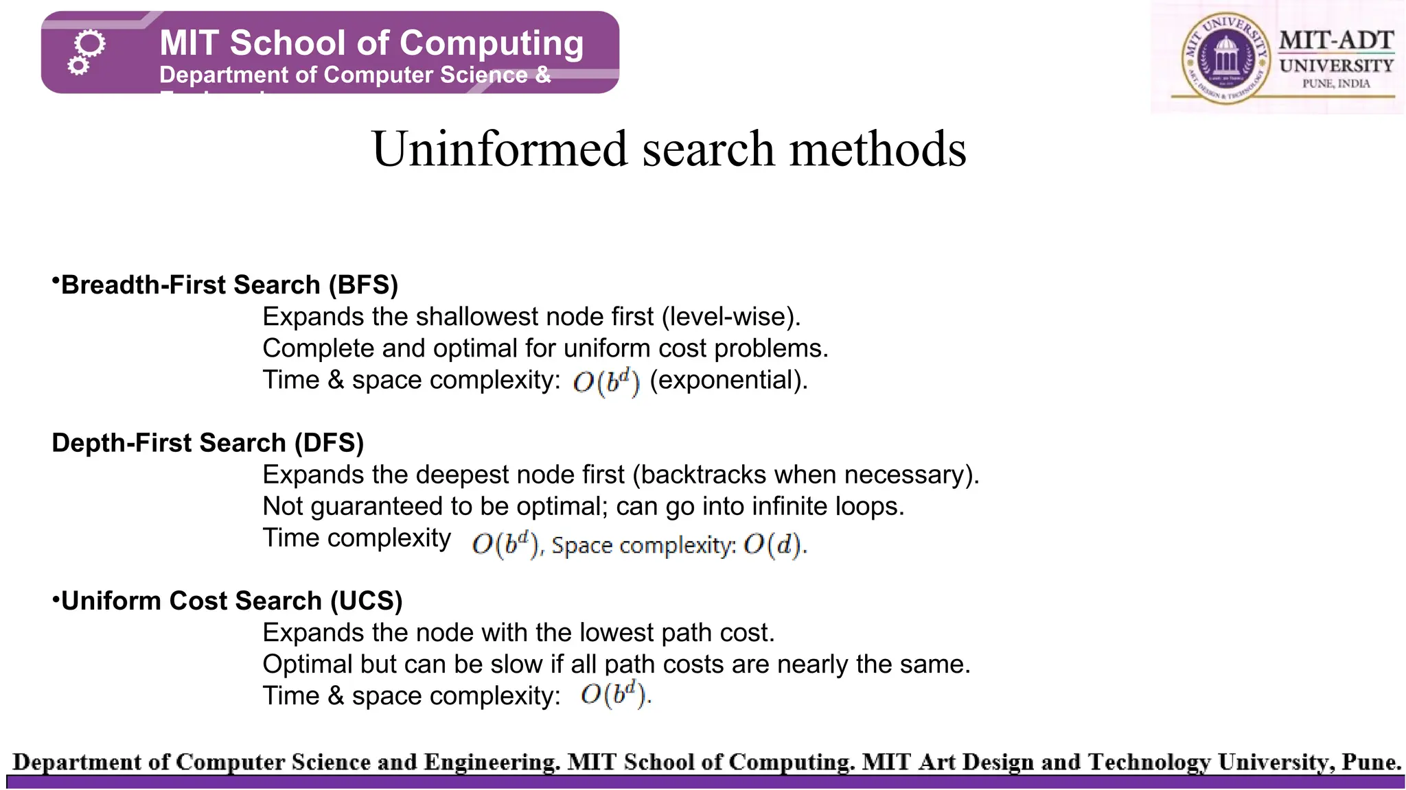
•Breadth-First Search (BFS)
Expands the shallowest node first (level-wise).
Complete and optimal for uniform cost problems.
Time & space complexity: (exponential).
Depth-First Search (DFS)
Expands the deepest node first (backtracks when necessary).
Not guaranteed to be optimal; can go into infinite loops.
Time complexity
•Uniform Cost Search (UCS)
Expands the node with the lowest path cost.
Optimal but can be slow if all path costs are nearly the same.
Time & space complexity:

Depth-Limited Search (DLS)
DFS with a depth limit to prevent infinite loops.
Not always complete; may not find a solution if the limit is too low.
Iterative Deepening Depth-First Search (IDDFS)
Repeatedly applies DFS with increasing depth limits.
Completeness and optimality like BFS, but lower space complexity.

• How BFS Works:
• Start from an initial node (root).
• Expand all neighboring nodes before moving deeper.
• Use a queue (FIFO - First In, First Out) to keep track of nodes.
• Continue exploring until the goal node is found or all nodes are
visited
Breadth-First Search (BFS)
Engineering

Engineering
BFS Traversal Starting from A:
1.Queue: [A]
2.Visit A → Enqueue [B, C]
3.Visit B → Enqueue [C, D, E]
4.Visit C → Enqueue [D, E, F]
5.Visit D → Enqueue [E, F]
6.Visit E → Enqueue [F]
7.Visit F → Queue empty, end traversal.
Output: A → B → C → D → E → F
Time & Space Complexity:
• Time Complexity: O(V+E) (Vertices + Edges)
• Space Complexity: O(V) (for storing visited nodes and queue)

Engineering
Properties of BSF :
Complete: Always finds a solution if one exists.
Optimal: Guarantees the shortest path in an unweighted graph.
High Memory Usage: Needs to store all nodes in memory.
Slow for Large Graphs: Explores all neighbors before moving deeper.

• It explores as deeply as possible along each branch before
backtracking, making it efficient for exploring large search spaces.
• How DFS Works:
• Start at the initial node (root).
• Explore one branch as deeply as possible before backtracking.
• Use a stack (LIFO - Last In, First Out) or recursion to track visited
nodes.
• Continue exploring until the goal node is found or all nodes are
visited.

DFS Traversal Starting from A (Pre-order):
1.Visit A → Push [C, B]
2.Visit B → Push [C, E, D]
3.Visit D → No neighbors left.
4.Backtrack to B → Visit E → No neighbors left.
5.Backtrack to A → Visit C → Push [F]
6.Visit F → No neighbors left.
Output (DFS Pre-order): A → B → D → E → C → F

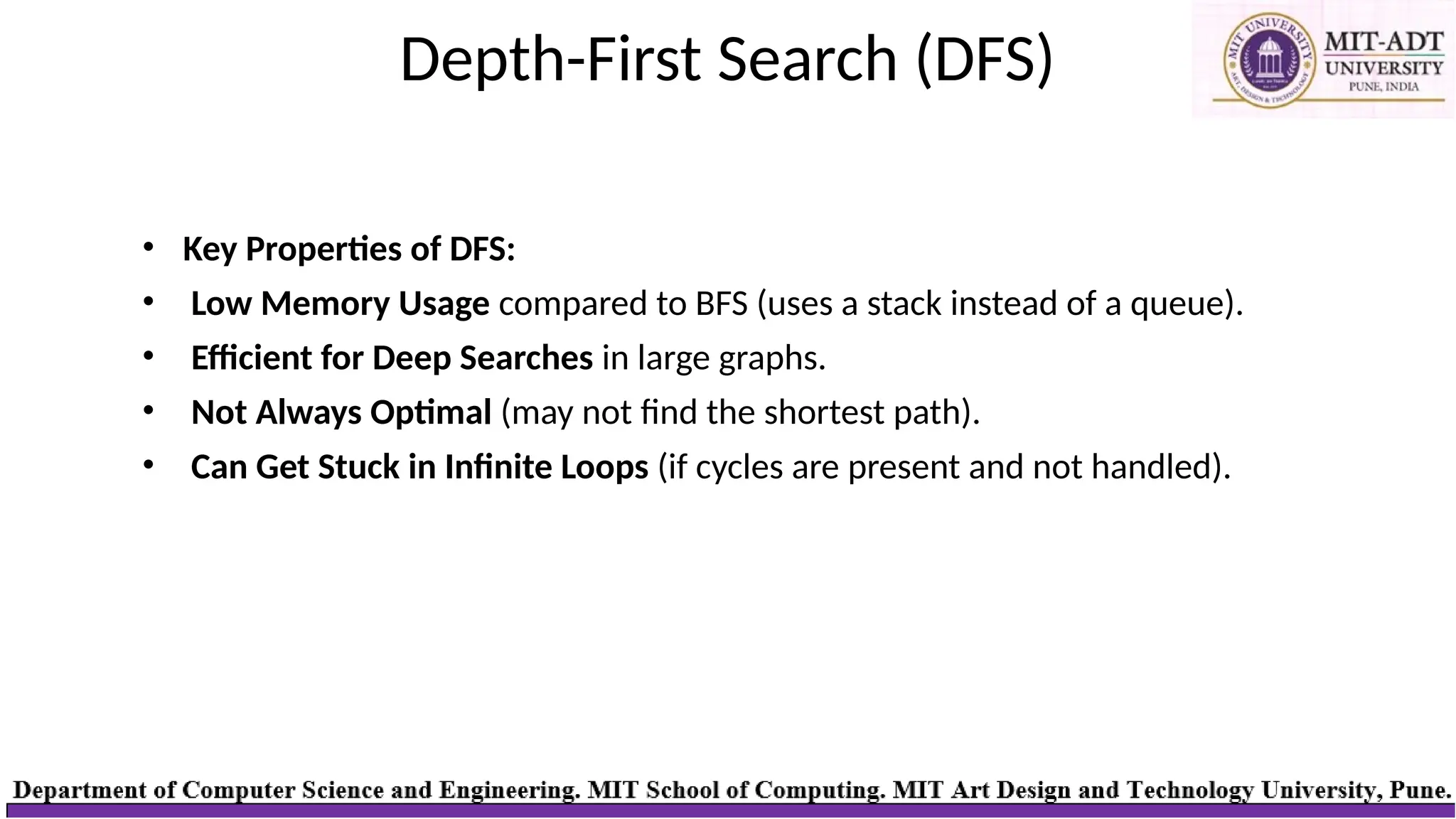
• Key Properties of DFS:
• Low Memory Usage compared to BFS (uses a stack instead of a queue).
• Efficient for Deep Searches in large graphs.
• Not Always Optimal (may not find the shortest path).
• Can Get Stuck in Infinite Loops (if cycles are present and not handled).

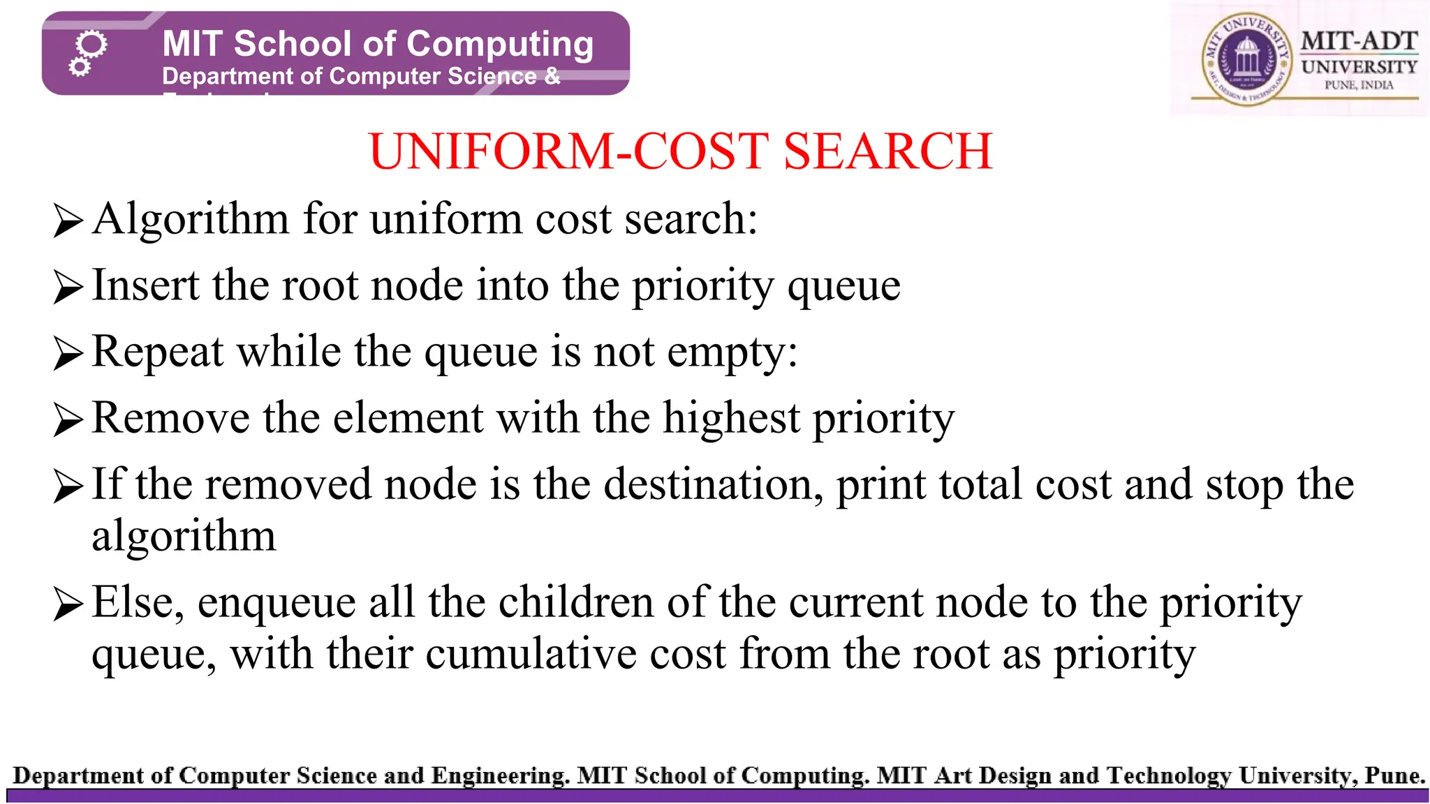
⮚Algorithm for uniform cost search:
⮚Insert the root node into the priority queue
⮚Repeat while the queue is not empty:
⮚Remove the element with the highest priority
⮚If the removed node is the destination, print total cost and stop the
algorithm
⮚Else, enqueue all the children of the current node to the priority
queue, with their cumulative cost from the root as priority
UNIFORM-COST SEARCH
Engineering

UNIFORM-COST SEARCH
Engineering

UNIFORM-COST SEARCH
Engineering
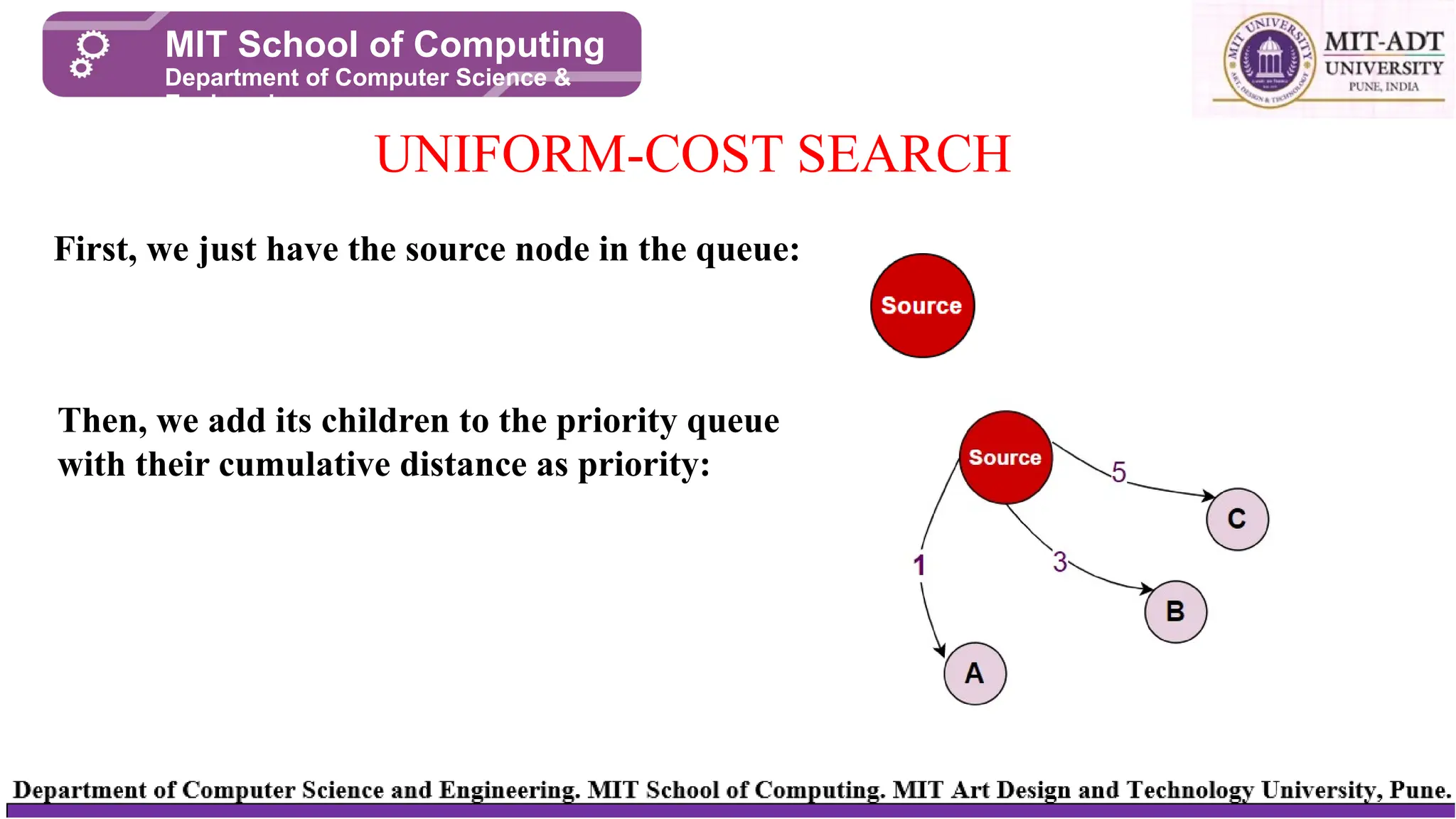
First, we just have the source node in the queue:
Then, we add its children to the priority queue
with their cumulative distance as priority:

UNIFORM-COST SEARCH
Engineering
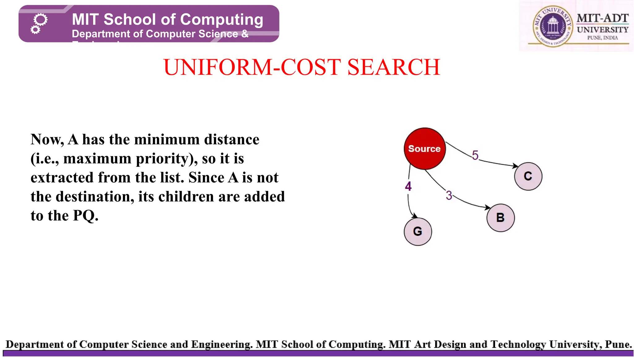
Now, A has the minimum distance
(i.e., maximum priority), so it is
extracted from the list. Since A is not
the destination, its children are added
to the PQ.

UNIFORM-COST SEARCH
Engineering
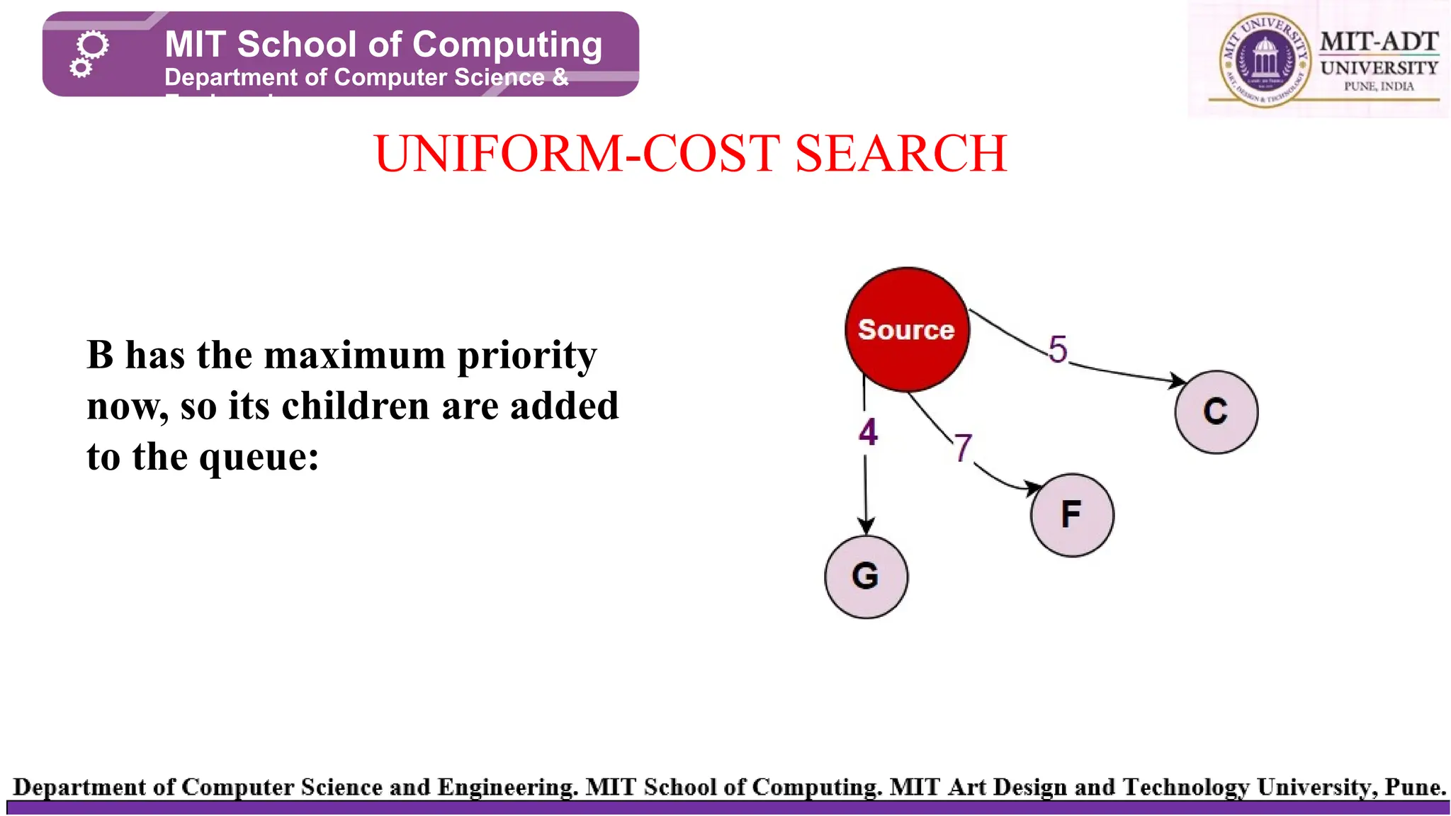
B has the maximum priority
now, so its children are added
to the queue:

UNIFORM-COST SEARCH
Engineering
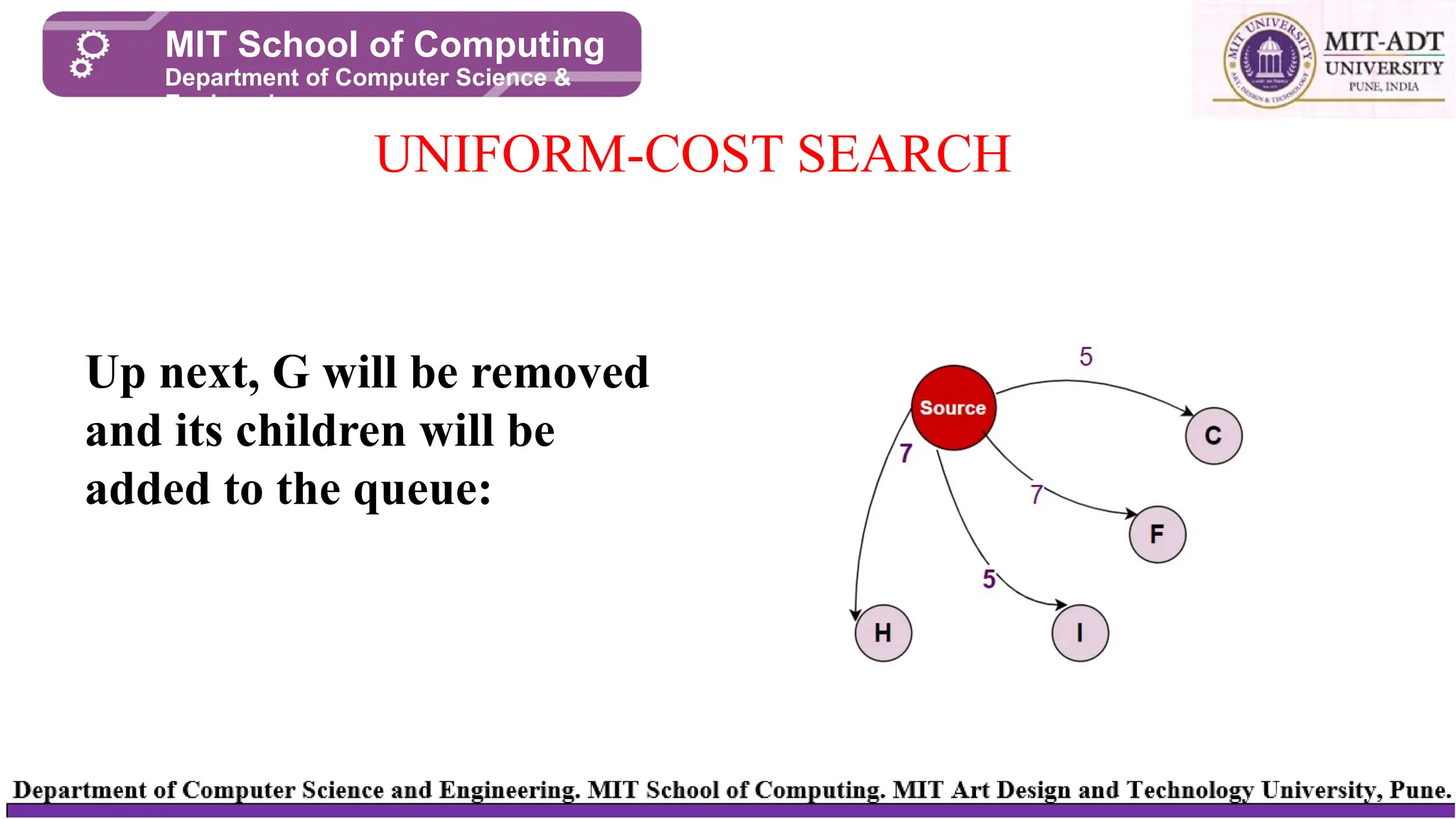
Up next, G will be removed
and its children will be
added to the queue:

UNIFORM-COST SEARCH
Engineering
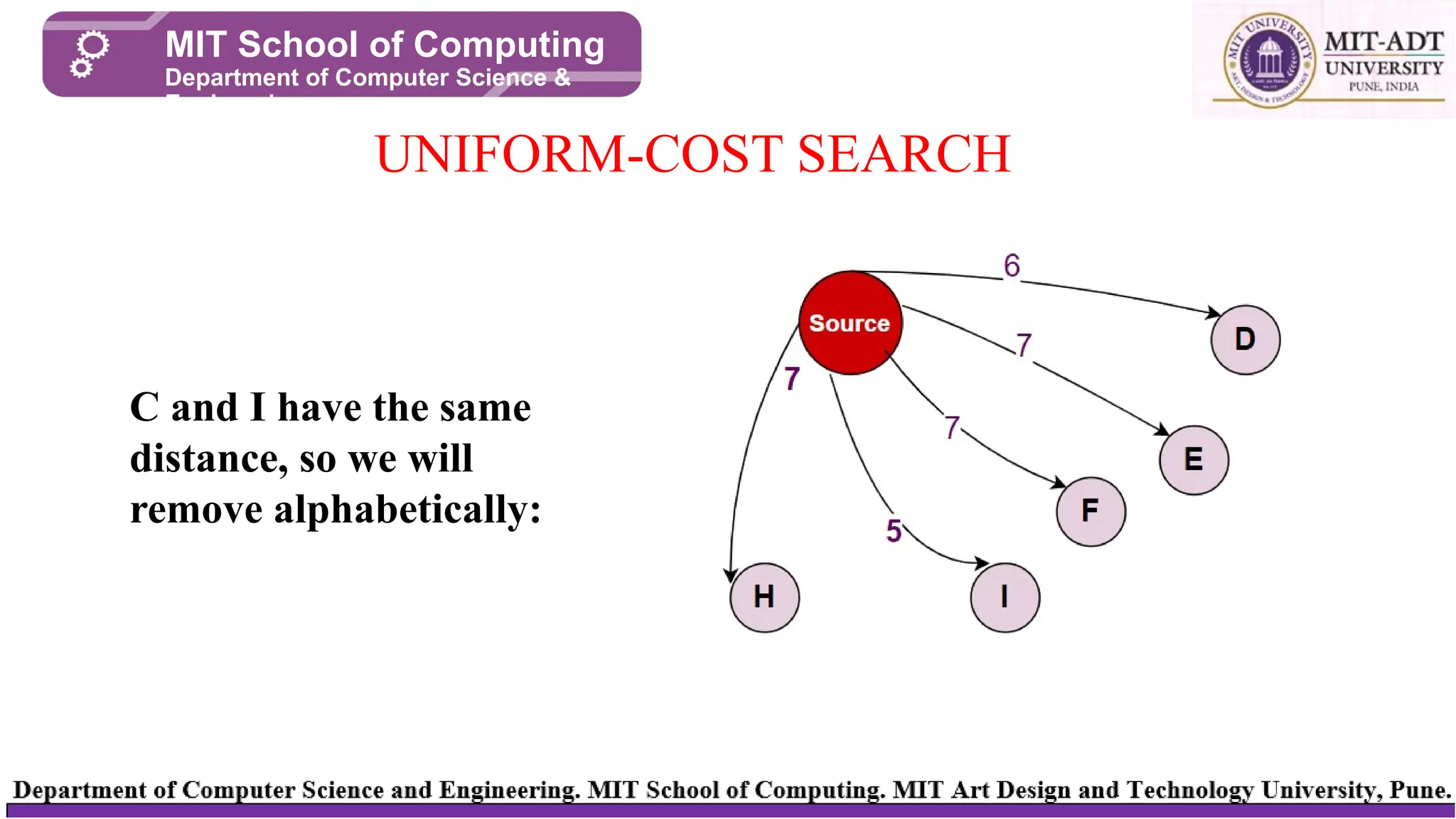
C and I have the same
distance, so we will
remove alphabetically:

UNIFORM-COST SEARCH
Engineering
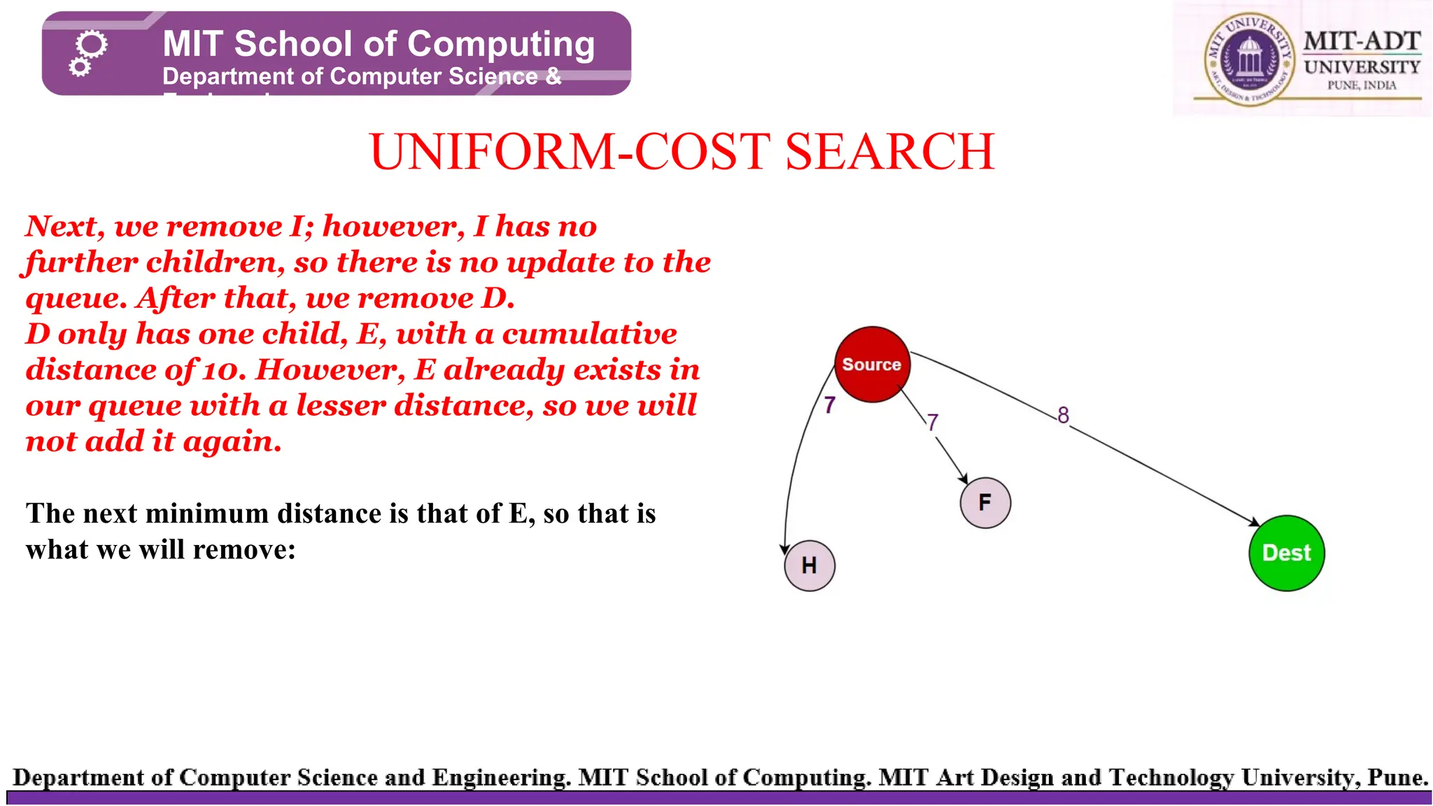
Next, we remove I; however, I has no
further children, so there is no update to the
queue. After that, we remove D.
D only has one child, E, with a cumulative
distance of 10. However, E already exists in
our queue with a lesser distance, so we will
not add it again.
The next minimum distance is that of E, so that is
what we will remove:

UNIFORM-COST SEARCH
Engineering
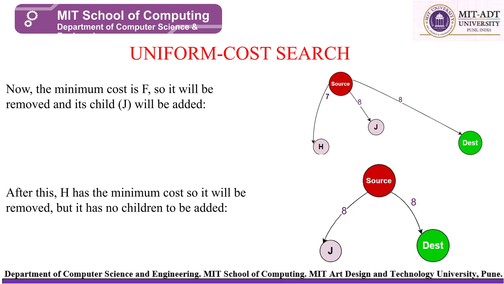
Now, the minimum cost is F, so it will be
removed and its child (J) will be added:
After this, H has the minimum cost so it will be
removed, but it has no children to be added:

UNIFORM-COST SEARCH
Engineering
Finally, we remove the Destination node, check that it is our target, and stop
the algorithm here.
The minimum distance between the source and destination nodes (i.e., 8) has
been found.

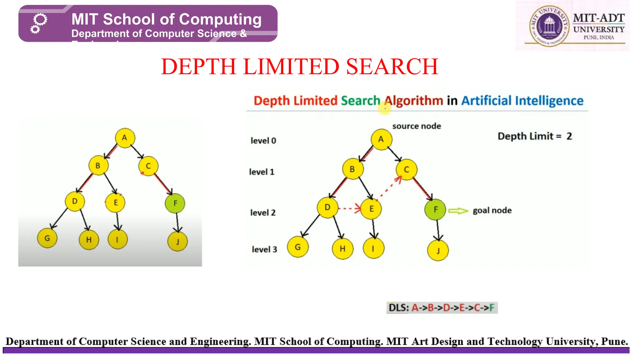
The depth-limited search (DLS) method is almost equal to depth-first search
(DFS), but DLS can work on the infinite state space problem because it bounds
the depth of the search tree with a predetermined limit L. Nodes at this depth
limit are treated as if they had no successors.
DEPTH LIMITED SEARCH
Engineering

DEPTH LIMITED SEARCH
Engineering

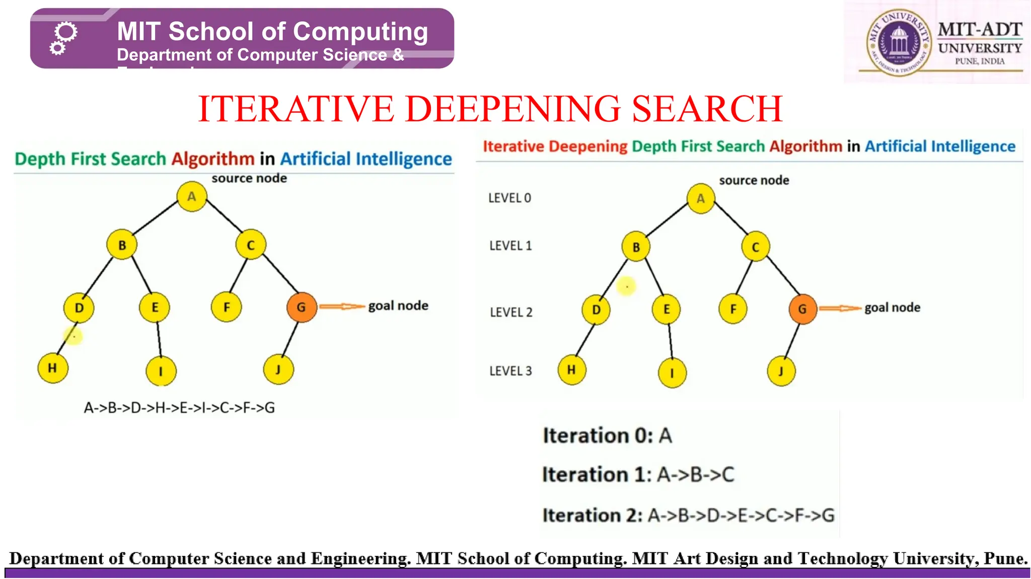
Iterative deepening search (or iterative deepening depth-first search) is a general
strategy, often used in combination with depth-limited search, that finds the best
depth limit. It does this by gradually increasing the limit—first 0, then 1, then 2,
and so on—until a goal is found. This will occur when the depth limit reaches d,
the depth of the shallowest goal node.
ITERATIVE DEEPENING SEARCH
Engineering

ITERATIVE DEEPENING SEARCH
Engineering

BIDIRECTIONAL SEARCH
Engineering
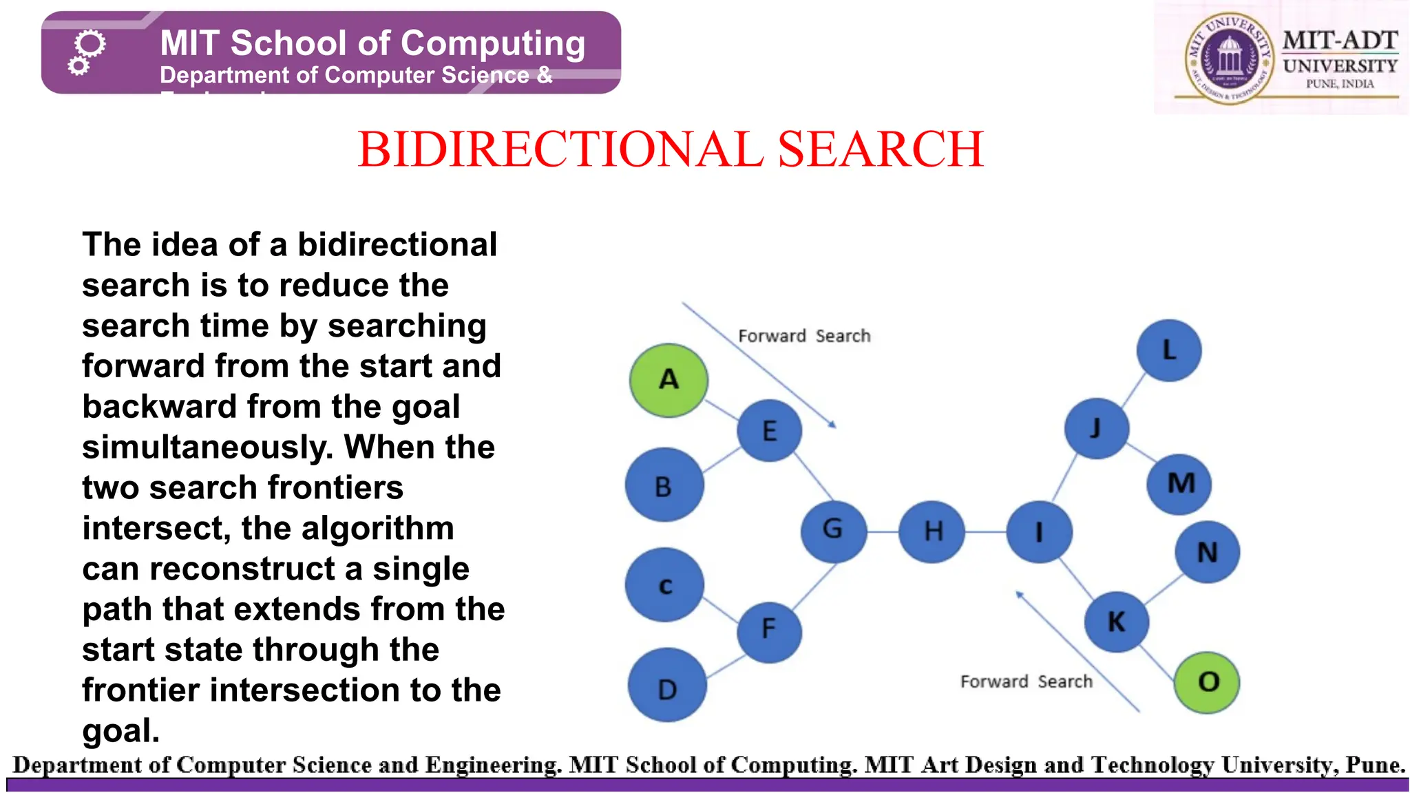
The idea of a bidirectional
search is to reduce the
search time by searching
forward from the start and
backward from the goal
simultaneously. When the
two search frontiers
intersect, the algorithm
can reconstruct a single
path that extends from the
start state through the
frontier intersection to the
goal.

⮚ Step 1: Say, A is the initial node and O is the goal node, and H is the intersection node.
⮚ Step 2: We will start searching simultaneously from start to goal node and backward from goal to
start node.
⮚ Step 3: Whenever the forward search and backward search intersect at one node, then the
searching stops.
Advantages
Below are the advantages:
• One of the main advantages of bidirectional searches is the speedat which we get the desired
results.
• It drastically reduces the time taken by the search by having simultaneous searches.
• It also saves resources for users as it requires less memory capacity to store all the searches.
Engineering

Disadvantages
⮚ The fundamental issue with bidirectional search is that the user should be
aware of the goal state to use bidirectional search and thereby to decrease its
use cases drastically.
⮚ The algorithm must be robust enough to understand the intersection when the
search should come to an end or else there’s a possibility of an infinite loop.
⮚ It is also not possible to search backwards through all states.
Engineering

Informed Search Strategies
• Informed search strategies employ knowledge about the problem
domain to guide the search process. They utilize heuristics, which
are rules of thumb that estimate the distance to the goal.
• These heuristics provide valuable insights, enabling the algorithm to
prioritize paths that are likely to lead to the optimal solution. This
strategy contrasts with uninformed search algorithms, which explore
the search space blindly.

Greedy Best first Search
• Greedy best-first search algorithm always selects the path
which appears best at that moment.
• It is the combination of depth-first search and breadth-first
search algorithms. It uses the heuristic function and search.
• Best-first search allows us to take the advantages of both
algorithms.
• With the help of best-first search, at each step, we can choose the
most promising node.

Greedy Best first Search
• In the best first search algorithm, we expand the node which is
closest to the goal node and the closest cost is estimated by
heuristic function, i.e.
• f(n)= g(n).
•Were, h(n)= estimated cost from node n to the goal.
•The greedy best first algorithm is implemented by the priority
queue.

Greedy BFS Algorithm
• Step 1: Place the starting node into the OPEN list.
• Step 2: If the OPEN list is empty, Stop and return failure.
• Step 3: Remove the node n, from the OPEN list which has the lowest value of
h(n), and places it in the CLOSED list.
• Step 4: Expand the node n, and generate the successors of node n.
• Step 5: Check each successor of node n, and find whether any node is a goal
node or not. If any successor node is goal node, then return success and
terminate the search, else proceed to Step 6.
• Step 6: For each successor node, algorithm checks for evaluation function f(n),
and then check if the node has been in either OPEN or CLOSED list. If the node
has not been in both list, then add it to the OPEN list.
• Step 7: Return to Step 2.

Greedy BFS Algorithm
• Advantages:
– Best first search can switch between BFS and DFS by gaining the
advantages of both the algorithms.
– This algorithm is more efficient than BFS and DFS algorithms.
• Disadvantages:
– It can behave as an unguided depth-first search in the worst case
scenario.
– It can get stuck in a loop as DFS.
– This algorithm is not optimal.

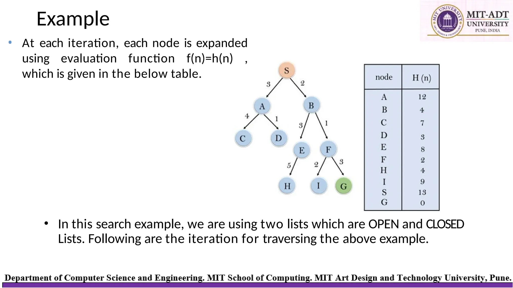
Example
• In this search example, we are using two lists which are OPEN and CLOSED
Lists. Following are the iteration for traversing the above example.
• At each iteration, each node is expanded
using evaluation function f(n)=h(n) ,
which is given in the below table.

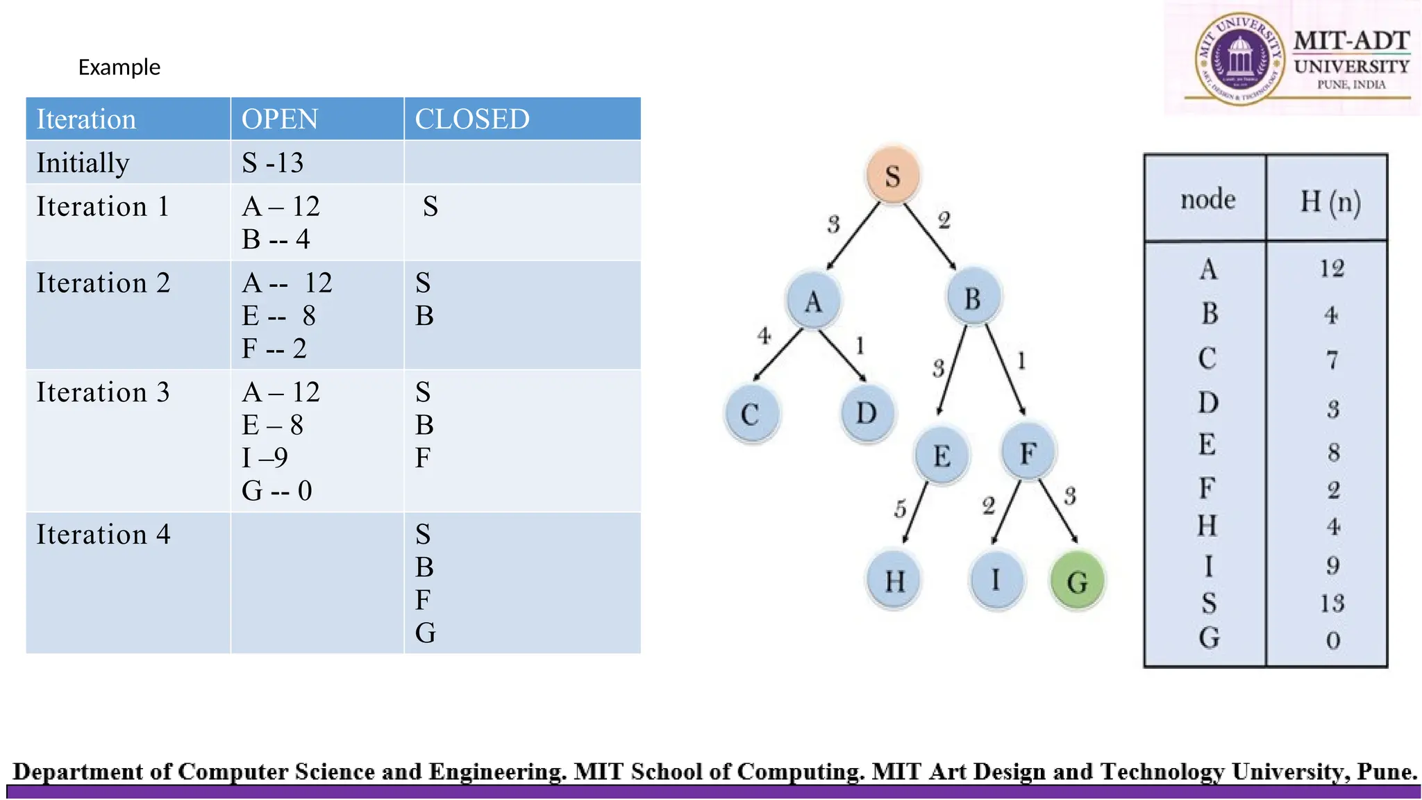
Example
Iteration OPEN CLOSED
Initially S -13
Iteration 1 A – 12
B -- 4
S
Iteration 2 A -- 12
E -- 8
F -- 2
S
B
Iteration 3 A – 12
E – 8
I –9
G -- 0
S
B
F
Iteration 4 S
B
F
G

Example :
S
A B C
D H
F G
E
10
9 7 8
8
6
6
3
0

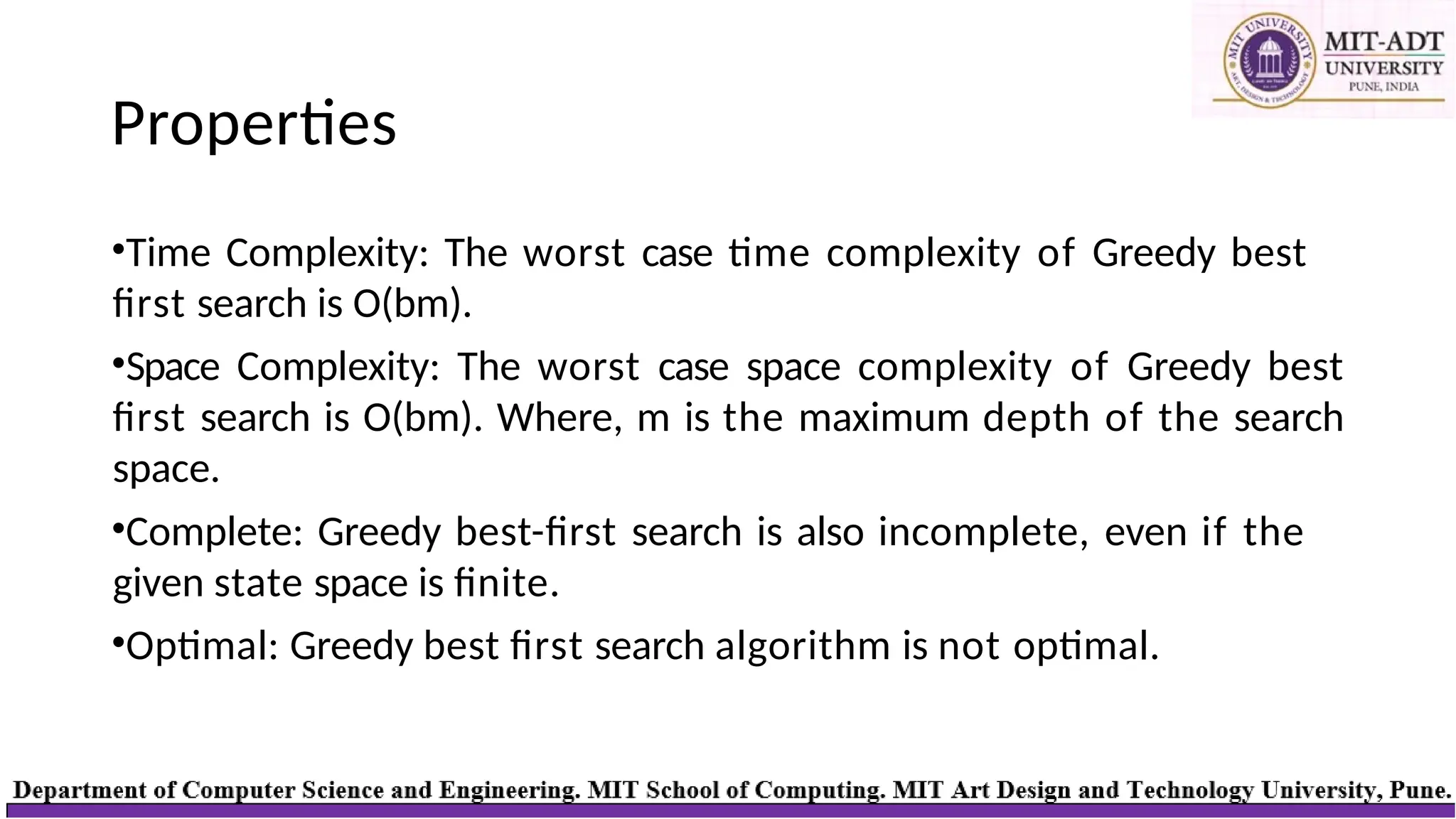
Properties
•Time Complexity: The worst case time complexity of Greedy best
first search is O(bm).
•Space Complexity: The worst case space complexity of Greedy best
first search is O(bm). Where, m is the maximum depth of the search
space.
•Complete: Greedy best-first search is also incomplete, even if the
given state space is finite.
•Optimal: Greedy best first search algorithm is not optimal.

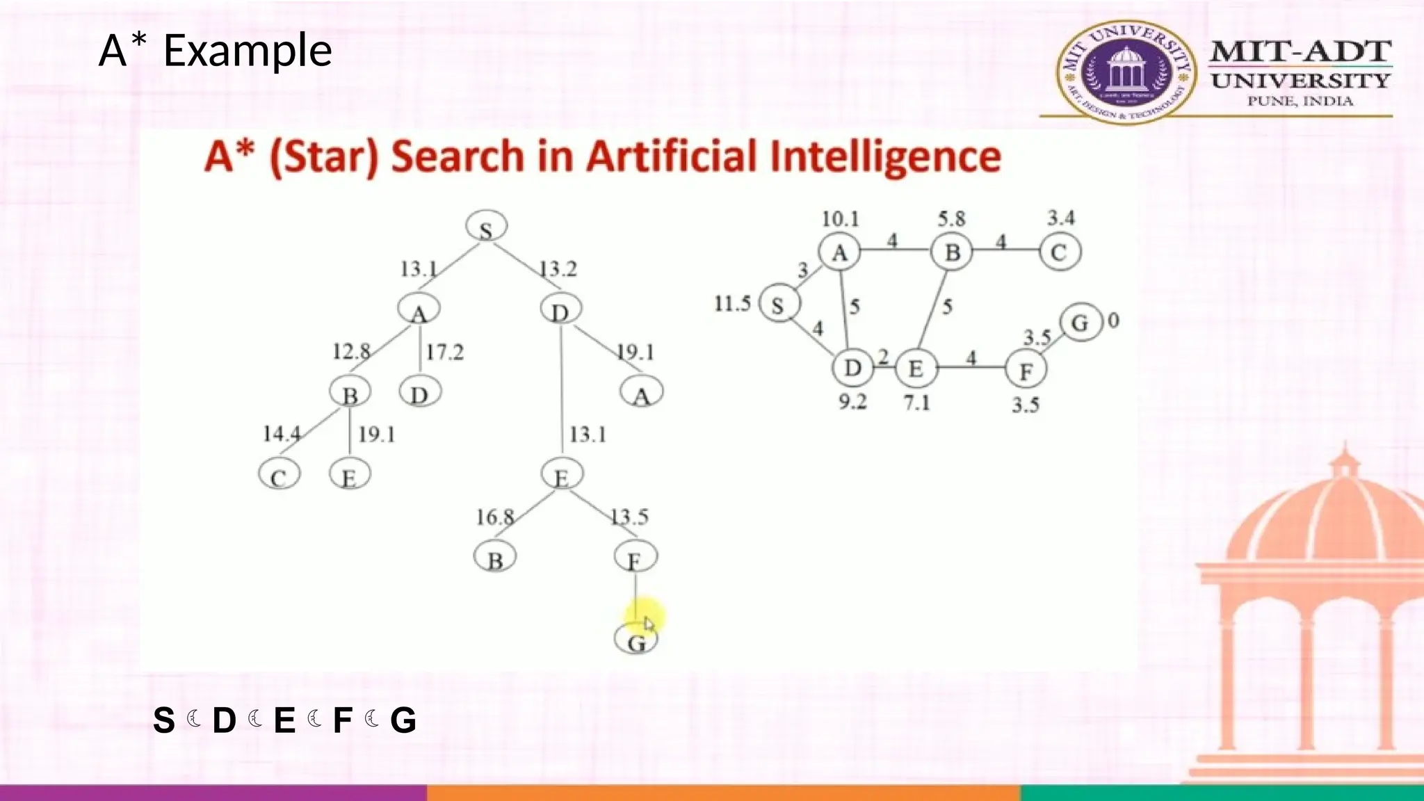
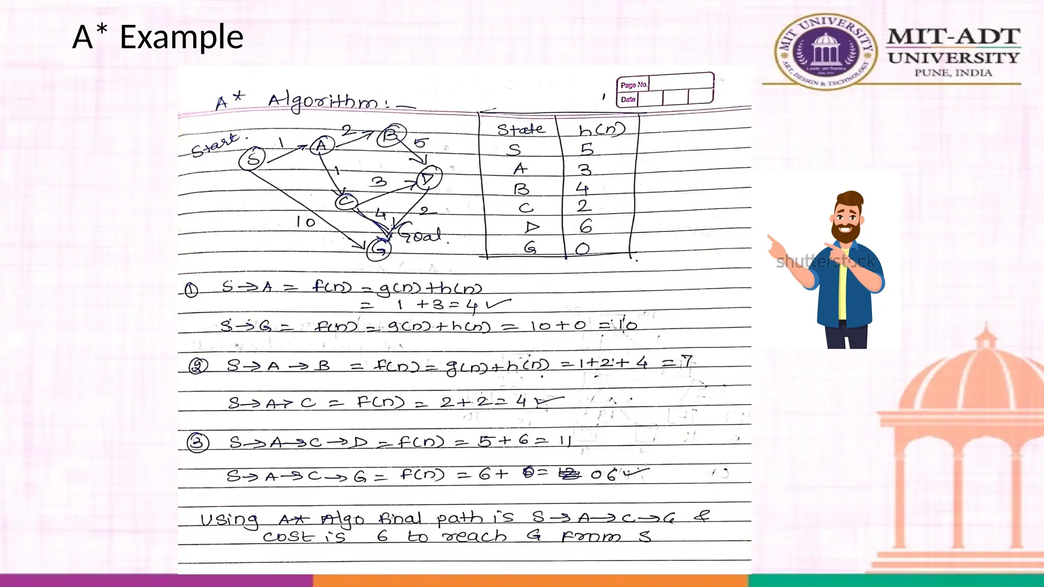
What is A* Search Algorithm?
• Moving from one place to another is a task we do almost
everyday.
• Finding the shortest path by ourselves was difficult.
• We now have algorithms that help us find that shortest route.
A* is one the most popular algorithms out there.

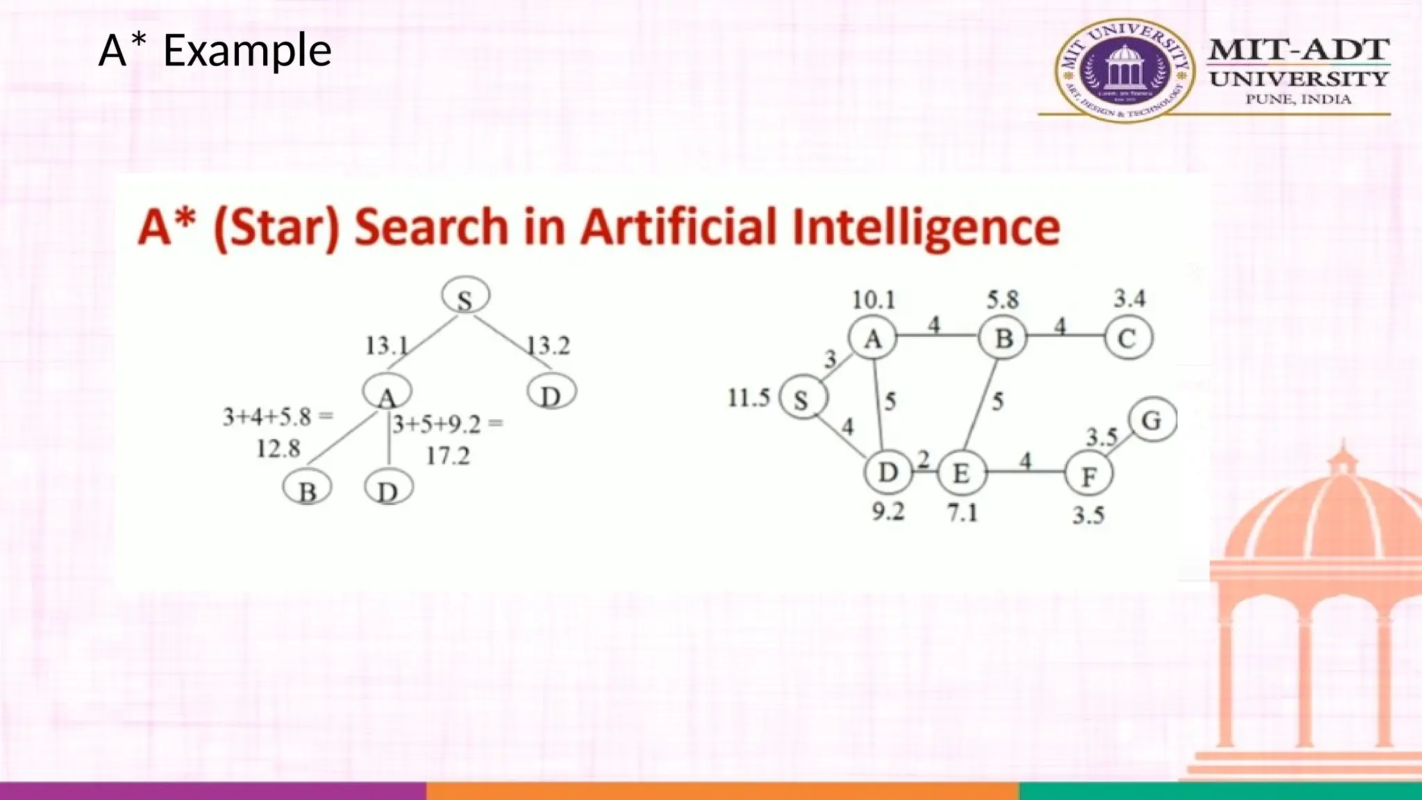
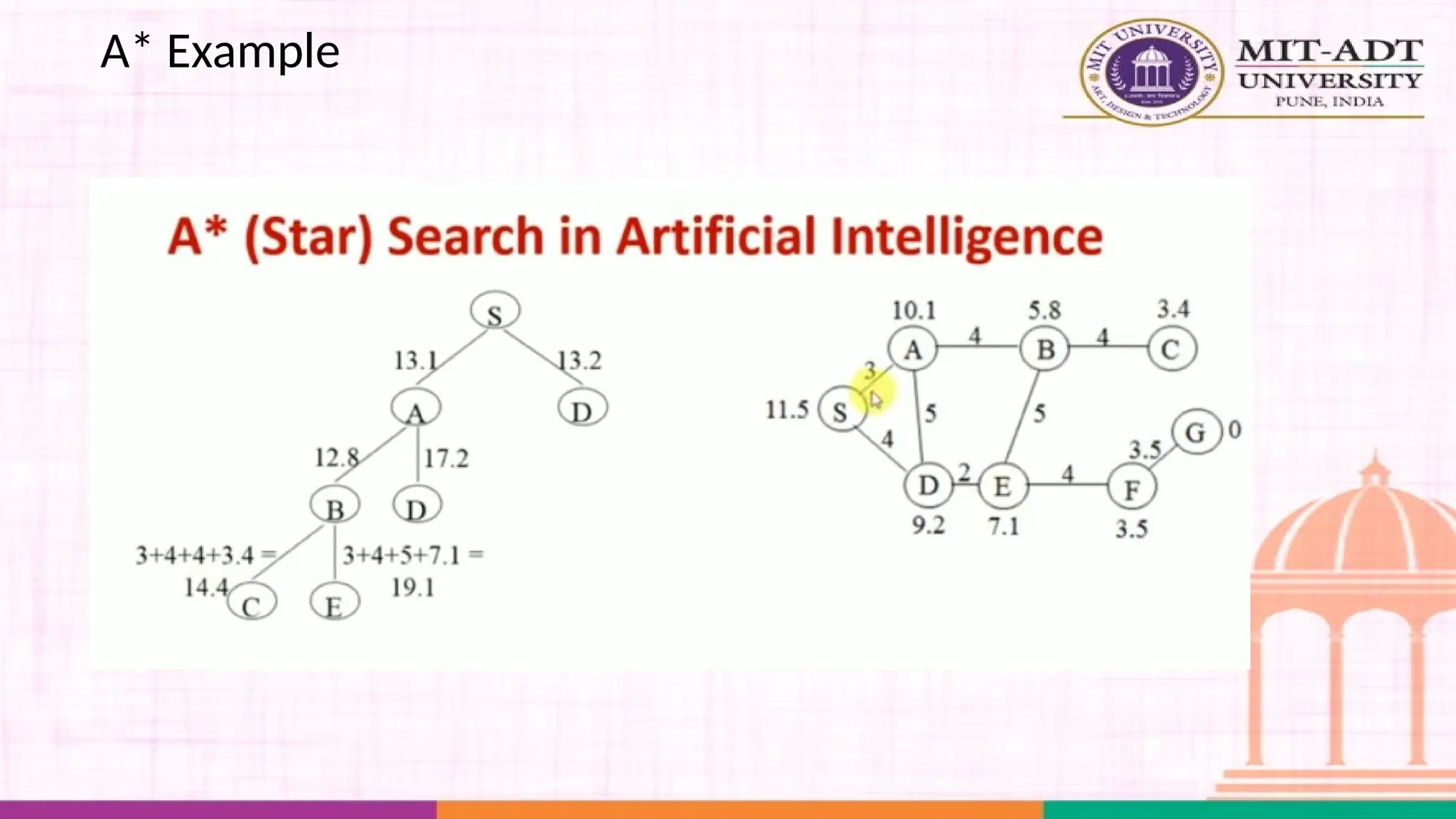
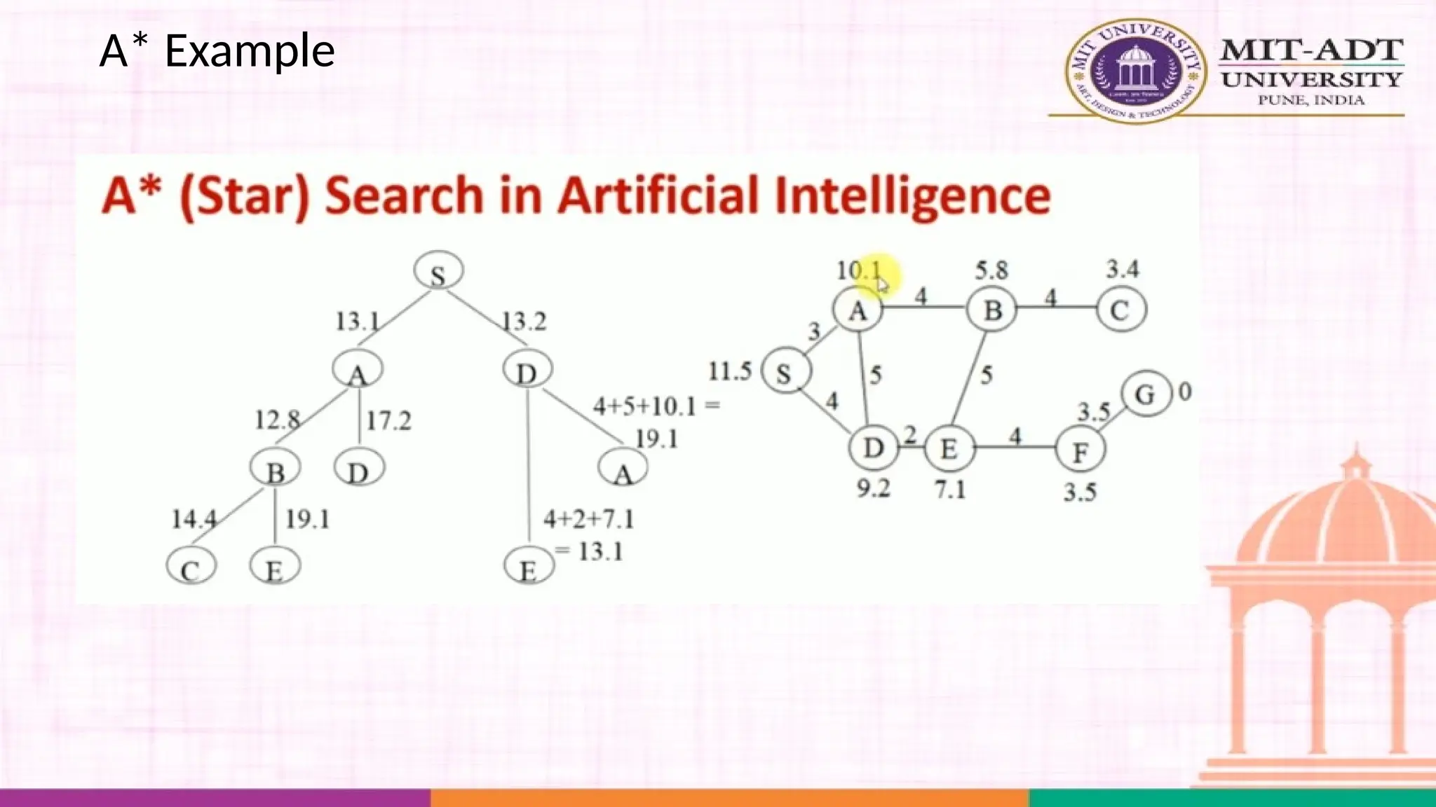
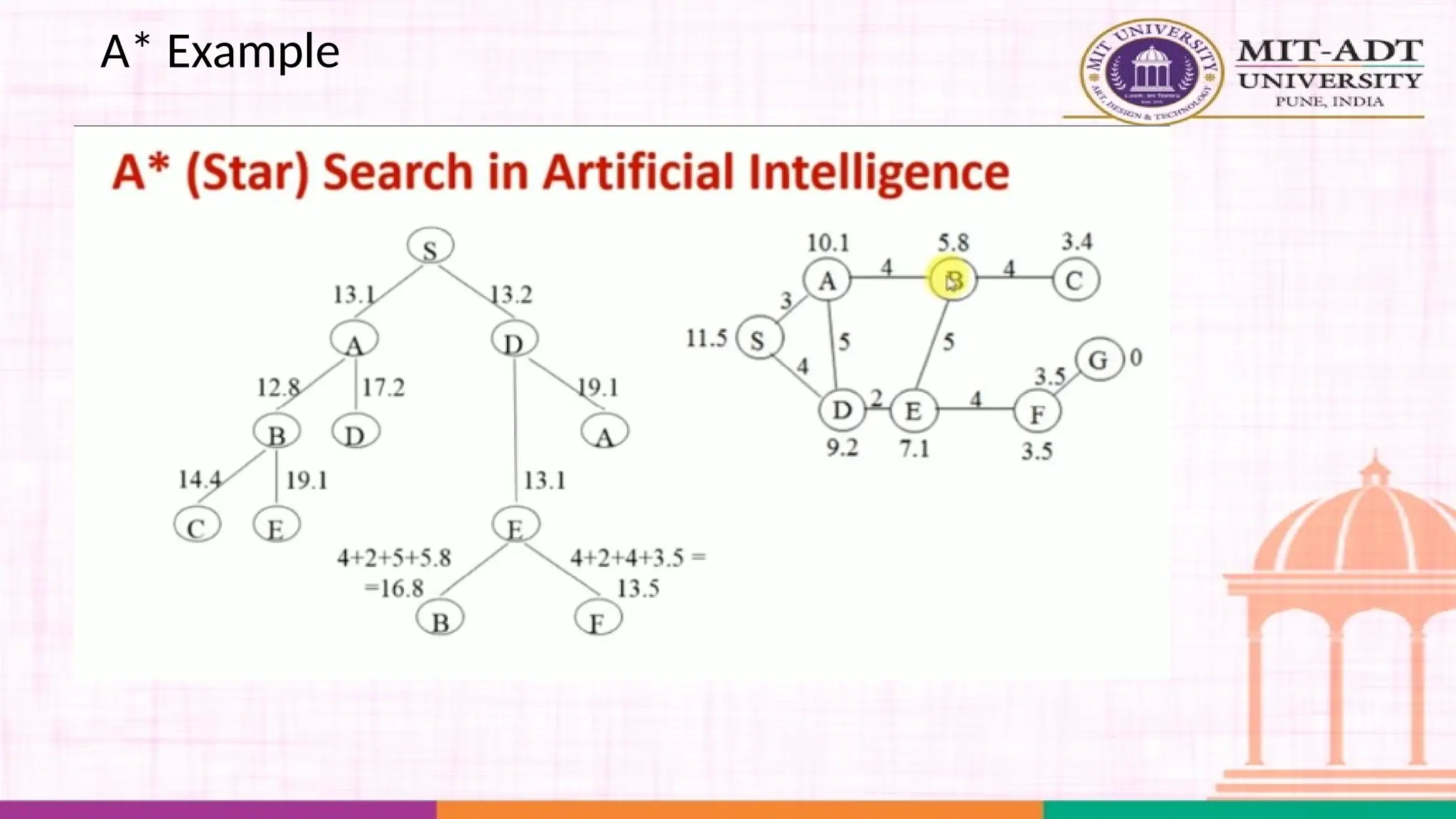
What is A* Algorithm?
It is an advanced BFS algorithm that searches for shorter paths first rather than
the longer paths. A* is optimal as well as a complete algorithm.
Complete
Optimal
A* is going to find all the paths that are available to us from
the source to the destination
A* is sure to find the least cost from the source to the
destination
So that makes A* the best algorithm right? YES.
But A* is slow and also the space it requires is a lot as it saves all the possible
paths that are available to us. This makes other faster algorithms have an upper
hand over A* but it is nevertheless, one of the best algorithms out there.

updated UNIT 2.pptxEWDSKJL;MSDCL;MLDSPKDPS

More Related Content

Similar to updated UNIT 2.pptxEWDSKJL;MSDCL;MLDSPKDPS

Recently uploaded

updated UNIT 2.pptxEWDSKJL;MSDCL;MLDSPKDPS