Linear algebra has many applications including understanding networks and graphs, modeling complex systems like bridges and molecules, quantum computing, chaos theory, coding and error correction, data compression, and solving systems of equations. It can be used to analyze vibrations, study dynamical systems, and efficiently solve Lagrange multiplier systems.
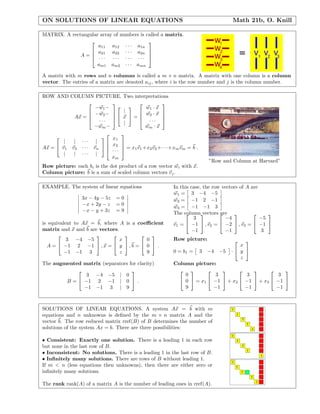
![USE OF LINEAR ALGEBRA (III) Math 21b, Oliver Knill
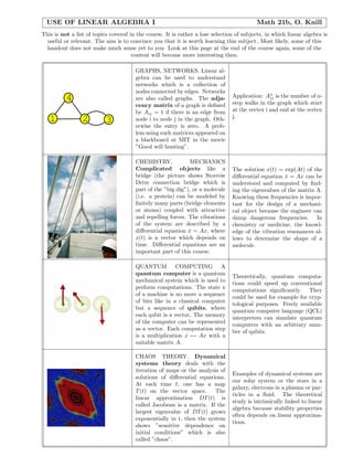
STATISTICS When analyzing data
statistically, one often is interested
in the correlation matrix Aij = For example, if the random variables
E[Yi Yj ] of a random vector X = have a Gaussian (=Bell shaped) dis-
(X1 , . . . , Xn ) with Yi = Xi − E[Xi ]. tribution, the correlation matrix to-
This matrix is derived from the data gether with the expectation E[Xi ]
and determines often the random determines the random variables.
variables when the type of the dis-
tribution is fixed.
A famous example is the prisoner
dilemma. Each player has the
choice to corporate or to cheat.. The
game is described by a 2x2 matrix
3 0
like for example . If a
5 1
GAME THEORY Abstract Games player cooperates and his partner
are often represented by pay-off ma- also, both get 3 points. If his partner
trices. These matrices tell the out- cheats and he cooperates, he gets 5
come when the decisions of each points. If both cheat, both get 1
player are known. point. More generally, in a game
with two players where each player
can chose from n strategies, the pay-
off matrix is a n times n matrix
A. A Nash equilibrium is a vector
p ∈ S = { i pi = 1, pi ≥ 0 } for
which qAp ≤ pAp for all q ∈ S.
NEURAL NETWORK In part of
neural network theory, for exam-
ple Hopfield networks, the state
space is a 2n-dimensional vector
space. Every state of the network
is given by a vector x, where each
For example, if Wij = xi yj , then x
component takes the values −1 or
is a fixed point of the learning map.
1. If W is a symmetric nxn matrix,
one can define a ”learning map”
T : x → signW x, where the sign
is taken component wise. The en-
ergy of the state is the dot prod-
uct −(x, W x)/2. One is interested
in fixed points of the map.](https://image.slidesharecdn.com/6493617/85/Harvard_University_-_Linear_Al-3-320.jpg)

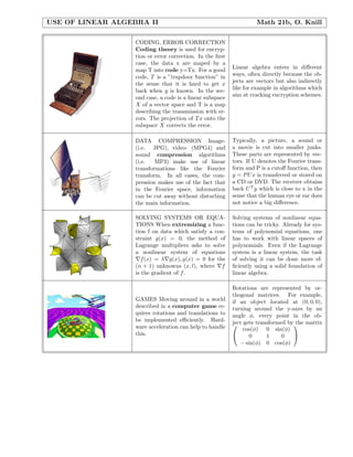
![SOLUTION TO 2). [L2 ]ij is by definition of the matrix product the sum Li1 L1j + Li2 L2j +
... + Li4 Lhj . Each term Li1 L1j is 1 if and only if there is a path of length 2 going from i to j
passing through k. Therefore [L2 ]ij is the number of paths of length 2 going from node i to j.
Similarly, [Ln ]ij is the number of paths of length n going from i to j. The answer is
2 7 2 3
7 2 12 7
L3 =
2 12 0 2
3 7 2 2
SOLUTION TO 3). The geometric series formula
xn = (1 − x)−1
n
holds also for matrices:
∞ ∞
f (z) = [Ln ]ij z n = [ Ln z n )]ij = (1 − Lz)−1
n=0 n=0
Cramers formula for the inverse of a matrix which involves the determinant
A−1 = det(Aij )/det(A)
This leads to an explicit formula
det(1 − zLij )/det(1 − zL)
which can also be written as
det(Lij − z)/det(L − z) .
SOLUTION TO 4). This is the special case, when i = 1 and j = 3.
1 −z 1
det(L − z) = det( 0 2 0 ) = −2 − z + 3z 2 − z 3 .
1 1 −z
−z 1 0 1
1 −z 2 1
det(L − z) = = 4 − 2z − 7z 2 + z 4
0 2 −z 0
1 1 0 −z
The final result is
(z 3 + 3z 2 − z − 2)/(z 4 − 7z 2 − 2z + 4) .](https://image.slidesharecdn.com/6493617/85/Harvard_University_-_Linear_Al-6-320.jpg)
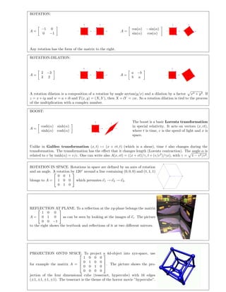
![LINEAR EQUATIONS Math 21b, O. Knill
SYSTEM OF LINEAR EQUATIONS. A collection of linear equations is called a system of linear equations.
An example is
3x − y − z = 0
−x + 2y − z = 0 .
−x − y + 3z = 9
It consists of three equations for three unknowns x, y, z. Linear means that no nonlinear terms like
x2 , x3 , xy, yz 3 , sin(x) etc. appear. A formal definition of linearity will be given later.
LINEAR EQUATION. More precicely, ax + by = c is the general linear equation in two variables. ax +
by + cz = d is the general linear equation in three variables. The general linear equation in n variables is
a1 x1 + a2 x2 + ... + an xn = 0 Finitely many such equations form a system of linear equations.
SOLVING BY ELIMINATION.
Eliminate variables. In the example the first equation gives z = 3x − y. Putting this into the second and
third equation gives
−x + 2y − (3x − y) =0
−x − y + 3(3x − y) =9
or
−4x + 3y = 0
.
8x − 4y = 9
The first equation gives y = 4/3x and plugging this into the other equation gives 8x − 16/3x = 9 or 8x = 27
which means x = 27/8. The other values y = 9/2, z = 45/8 can now be obtained.
SOLVE BY SUITABLE SUBTRACTION.
Addition of equations. If we subtract the third equation from the second, we get 3y − 4z = −9 and add
three times the second equation to the first, we get 5y − 4z = 0. Subtracting this equation to the previous one
gives −2y = −9 or y = 2/9.
SOLVE BY COMPUTER.
Use the computer. In Mathematica:
Solve[{3x − y − z == 0, −x + 2y − z == 0, −x − y + 3z == 9}, {x, y, z}] .
But what did Mathematica do to solve this equation? We will look in this course at some efficient algorithms.
GEOMETRIC SOLUTION.
Each of the three equations represents a plane in
three-dimensional space. Points on the first plane
satisfy the first equation. The second plane is the
solution set to the second equation. To satisfy the
first two equations means to be on the intersection
of these two planes which is here a line. To satisfy
all three equations, we have to intersect the line with
the plane representing the third equation which is a
point.
LINES, PLANES, HYPERPLANES.
The set of points in the plane satisfying ax + by = c form a line.
The set of points in space satisfying ax + by + cd = d form a plane.
The set of points in n-dimensional space satisfying a 1 x1 + ... + an xn = a0 define a set called a hyperplane.](https://image.slidesharecdn.com/6493617/85/Harvard_University_-_Linear_Al-7-320.jpg)


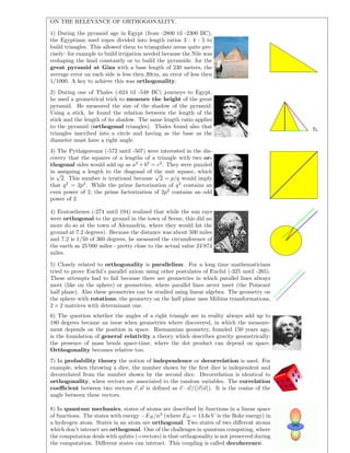
![LINEAR TRANSFORMATIONS Math 21b, O. Knill
TRANSFORMATIONS. A transformation T from a set X to a set Y is a rule, which assigns to every element
in X an element y = T (x) in Y . One calls X the domain and Y the codomain. A transformation is also called
a map.
LINEAR TRANSFORMATION. A map T from Rn to Rm is called a linear transformation if there is a
m × n matrix A such that
T (x) = Ax .
EXAMPLES.
3 4
• To the linear transformation T (x, y) = (3x+4y, x+5y) belongs the matrix . This transformation
1 5
maps the plane onto itself.
• T (x) = −3x is a linear transformation from the real line onto itself. The matrix is A = [−3].
• To T (x) = y · x from R3 to R belongs the matrix A = y = y1 y2 y3 . This 1 × 3 matrix is also called
a row vector. If the codomain is the real axes, one calls the map also a function. function defined on
space.
y1
• T (x) = xy from R to R3 . A = y = y2 is a 3 × 1 matrix which is also called a column vector. The
y3
map defines a line in space.
1 0
• T (x, y, z) = (x, y) from R3 to R2 , A is the 2 × 3 matrix A = 0 1 . The map projects space onto a
0 0
plane.
1 1 2
• To the map T (x, y) = (x + y, x − y, 2x − 3y) belongs the 3 × 2 matrix A = . The image
1 −1 −3
of the map is a plane in three dimensional space.
• If T (x) = x, then T is called the identity transformation.
PROPERTIES OF LINEAR TRANSFORMATIONS. T (0) = 0 T (x + y) = T (x) + T (y) T (λx) = λT (x)
In words: Linear transformations are compatible with addition and scalar multiplication. It does not matter,
whether we add two vectors before the transformation or add the transformed vectors.
ON LINEAR TRANSFORMATIONS. Linear transformations generalize the scaling transformation x → ax in
one dimensions.
They are important in
• geometry (i.e. rotations, dilations, projections or reflections)
• art (i.e. perspective, coordinate transformations),
• CAD applications (i.e. projections),
• physics (i.e. Lorentz transformations),
• dynamics (linearizations of general maps are linear maps),
• compression (i.e. using Fourier transform or Wavelet trans-
form),
• coding (many codes are linear codes),
• probability (i.e. Markov processes).
• linear equations (inversion is solving the equation)](https://image.slidesharecdn.com/6493617/85/Harvard_University_-_Linear_Al-13-320.jpg)


![THE INVERSE Math 21b, O. Knill
INVERTIBLE TRANSFORMATIONS. A map T from X
to Y is invertible if there is for every y ∈ Y a unique ⇒
point x ∈ X such that T (x) = y.
EXAMPLES.
1) T (x) = x3 is invertible from X = R to X = Y .
2) T (x) = x2 is not invertible from X = R to X = Y .
3) T (x, y) = (x2 + 3x − y, x) is invertible from X = R2 to Y = R2 .
4) T (x) = Ax linear and rref(A) has an empty row, then T is not invertible.
5) If T (x) = Ax is linear and rref(A) = 1n , then T is invertible.
INVERSE OF LINEAR TRANSFORMATION. If A is a n × n matrix and T : x → Ax has an inverse S, then
S is linear. The matrix A−1 belonging to S = T −1 is called the inverse matrix of A.
First proof: check that S is linear using the characterization S(a + b) = S(a) + S(b), S(λa) = λS(a) of linearity.
Second proof: construct the inverse using Gauss-Jordan elimination.
FINDING THE INVERSE. Let 1n be the n × n identity matrix. Start with [A|1n ] and perform Gauss-Jordan
elimination. Then
rref([A|1n ]) = 1n |A−1
Proof. The elimination process actually solves Ax = e i simultaneously. This leads to solutions vi which are the
columns of the inverse matrix A−1 because A−1 ei = vi .
2 6
EXAMPLE. Find the inverse of A = .
1 4
2 6 | 1 0
A | 12
1 4 | 0 1
1 3 | 1/2 0
.... | ...
1 4 | 0 1
1 3 | 1/2 0
.... | ...
0 1 | −1/2 1
1 0 | 2 −3
12 | A−1
0 1 | −1/2 1
2 −3
The inverse is A−1 = .
−1/2 1
THE INVERSE OF LINEAR MAPS R2 → R2 :
a b
If ad−bc = 0, the inverse of a linear transformation x → Ax with A =
c d
d −b
is given by the matrix A−1 = /(ad − bc).
−d a
SHEAR:
1 0 1 0
A= A−1 =
−1 1 1 1](https://image.slidesharecdn.com/6493617/85/Harvard_University_-_Linear_Al-17-320.jpg)
![DIAGONAL:
2 0 1/2 0
A= A−1 =
0 3 0 1/3
REFLECTION:
cos(2α) sin(2α) cos(2α) sin(2α)
A= A−1 = A =
sin(2α) − cos(2α) sin(2α) − cos(2α)
ROTATION:
cos(α) sin(α) cos(α) − sin(α)
A= A−1 =
− sin(α) cos(−α) sin(α) cos(α)
ROTATION-DILATION:
a −b a/r2 b/r 2
A= A−1 = , r 2 = a2 + b 2
b a −b/r 2 a/r2
BOOST:
cosh(α) sinh(α) cosh(α) − sinh(α)
A= A−1 =
sinh(α) cosh(α) − sinh(α) cosh(α)
1 0
NONINVERTIBLE EXAMPLE. The projection x → Ax = is a non-invertible transformation.
0 0
MORE ON SHEARS. The shears T (x, y) = (x + ay, y) or T (x, y) = (x, y + ax) in R 2 can be generalized. A
shear is a linear transformation which fixes some line L through the origin and which has the property that
T (x) − x is parallel to L for all x.
PROBLEM. T (x, y) = (3x/2 + y/2, y/2 − x/2) is a shear along a line L. Find L.
SOLUTION. Solve the system T (x, y) = (x, y). You find that the vector (1, −1) is preserved.
MORE ON PROJECTIONS. A linear map T with the property that T (T (x)) = T (x) is a projection. Examples:
T (x) = (y · x)y is a projection onto a line spanned by a unit vector y.
WHERE DO PROJECTIONS APPEAR? CAD: describe 3D objects using projections. A photo of an image is
a projection. Compression algorithms like JPG or MPG or MP3 use projections where the high frequencies are
cut away.
MORE ON ROTATIONS. A linear map T which preserves the angle between two vectors and the length of
each vector is called a rotation. Rotations form an important class of transformations and will be treated later
cos(φ) − sin(φ)
in more detail. In two dimensions, every rotation is of the form x → A(x) with A = .
sin(φ) cos(φ)
cos(φ) − sin(φ) 0
An example of a rotations in three dimensions are x → Ax, with A = sin(φ) cos(φ) 0 . it is a rotation
0 0 1
around the z axis.
MORE ON REFLECTIONS. Reflections are linear transformations different from the identity which are equal
to their own inverse. Examples:
−1 0 cos(2φ) sin(2φ)
2D reflections at the origin: A = , 2D reflections at a line A = .
0 1 sin(2φ) − cos(2φ)
−1 0 0 −1 0 0
3D reflections at origin: A = 0 −1 0 . 3D reflections at a line A = 0 −1 0 . By
0 0 −1 0 0 1
the way: in any dimensions, to a reflection at the line containing the unit vector u belongs the matrix [A] ij =
2(ui uj ) − [1n ]ij , because [B]ij = ui uj is the matrix belonging to the projection onto the line.
2
u1 − 1 u 1 u2 u1 u3
The reflection at a line containng the unit vector u = [u 1 , u2 , u3 ] is A = u2 u1 u2 − 1 u2 u3 .
2
u3 u1 u3 u2 u2 − 1
3
1 0 0
3D reflection at a plane A = 0 1 0 .
0 0 −1
Reflections are important symmetries in physics: T (time reflection), P (reflection at a mirror), C (change of
charge) are reflections. It seems today that the composition of TCP is a fundamental symmetry in nature.](https://image.slidesharecdn.com/6493617/85/Harvard_University_-_Linear_Al-18-320.jpg)
![MATRIX PRODUCT Math 21b, O. Knill
MATRIX PRODUCT. If B is a m × n matrix and A is a n × p matrix, then BA is defined as the m × p matrix
n
with entries (BA)ij = k=1 Bik Akj .
EXAMPLE. If B is a 3 × 4 matrix, and A is a 4 × 2 matrix then BA is a 3 × 2 matrix.
1 3 1 3
1 3 5 7 3 1 1 3 5 7 15 13
3 1 8 1 , A = , BA = 3 3 1
B= 1 0 1 8 1
1
= 14 11 .
0
1 0 9 2 1 0 9 2 10 5
0 1 0 1
COMPOSING LINEAR TRANSFORMATIONS. If S : Rm → Rn , x → Ax and T : Rn → Rp , y → By are
linear transformations, then their composition T ◦ S : x → B(A(x)) is a linear transformation from R m to Rp .
The corresponding matrix is the matrix product BA.
EXAMPLE. Find the matrix which is a composition of a rotation around the x-axes by an agle π/2 followed
by a rotation around the z-axes by an angle π/2.
SOLUTION. The first transformation has the property that e 1 → e1 , e2 → e3 , e3 → −e2 , the second e1 →
e2 , e2 → −e1 , e3 → e3 . If A is the matrix belonging to the first transformation and B the second, then BA
is the matrix to the composition. The composition maps 1 → −e2 → e3 → e1 is a rotation around a long
e
0 −1 0 1 0 0 0 0 1
diagonal. B = 1 0 0 A = 0 0 −1 , BA = 1 0 0 .
0 0 1 0 1 0 0 1 0
EXAMPLE. A rotation dilation is the composition of a rotation by α = arctan(b/a) and a dilation (=scale) by
√
r = a2 + b 2 .
REMARK. Matrix multiplication is a generalization of usual multiplication of numbers or the dot product.
MATRIX ALGEBRA. Note that AB = BA in general! Otherwise, the same rules apply as for numbers:
A(BC) = (AB)C, AA−1 = A−1 A = 1n , (AB)−1 = B −1 A−1 , A(B + C) = AB + AC, (B + C)A = BA + CA
etc.
PARTITIONED MATRICES. The entries of matrices can themselves be matrices. If B is a m × n matrix and
A is a n × p matrix, and assume the entries are k × k matrices, then BA is a m × p matrix where each entry
n
(BA)ij = k=1 Bik Akj is a k × k matrix. Partitioning matrices can be useful to improve the speed of matrix
multiplication (i.e. Strassen algorithm).
A11 A12
EXAMPLE. If A = , where Aij are k × k matrices with the property that A11 and A22 are
0 A22
A11 −A11 A12 A−1
−1 −1
22
invertible, then B = is the inverse of A.
0 A−122
APPLICATIONS. (The material which follows is for motivation puposes only, more applications appear in the
homework).
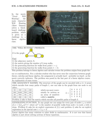
NETWORKS. Let us associate to the computer network (shown at the left) a
4
0 1 1 1
1 0 1 0
matrix
1 1 0 1 To a worm in the first computer we associate a vector
1 3
1 0 1 0
2
1
0
0 . The vector Ax has a 1 at the places, where the worm could be in the next
0
step. The vector (AA)(x) tells, in how many ways the worm can go from the first
computer to other hosts in 2 steps. In our case, it can go in three different ways
back to the computer itself.
Matrices help to solve combinatorial problems (see movie ”Good will hunting”).
For example, what does [A1000 ]22 tell about the worm infection of the network?
What does it mean if A100 has no zero entries?](https://image.slidesharecdn.com/6493617/85/Harvard_University_-_Linear_Al-19-320.jpg)
![FRACTALS. Closely related to linear maps are affine maps x → Ax + b. They are compositions of a linear
map with a translation. It is not a linear map if B(0) = 0. Affine maps can be disguised as linear maps
x A b Ax + b
in the following way: let y = and defne the (n+1)∗(n+1) matrix B = . Then By = .
1 0 1 1
Fractals can be constructed by taking for example 3 affine maps R, S, T which contract area. For a given object
Y0 define Y1 = R(Y0 ) ∪ S(Y0 ) ∪ T (Y0 ) and recursively Yk = R(Yk−1 ) ∪ S(Yk−1 ) ∪ T (Yk−1 ). The above picture
shows Yk after some iterations. In the limit, for example if R(Y 0 ), S(Y0 ) and T (Y0 ) are disjoint, the sets Yk
converge to a fractal, an object with dimension strictly between 1 and 2.
x 2x + 2 sin(x) − y
CHAOS. Consider a map in the plane like T : → We apply this map again and
y x
again and follow the points (x1 , y1 ) = T (x, y), (x2 , y2 ) = T (T (x, y)), etc. One writes T n for the n-th iteration
of the map and (xn , yn ) for the image of (x, y) under the map T n . The linear approximation of the map at a
2 + 2 cos(x) − 1 x f (x, y)
point (x, y) is the matrix DT (x, y) = . (If T = , then the row vectors of
1 y g(x, y)
DT (x, y) are just the gradients of f and g). T is called chaotic at (x, y), if the entries of D(T n )(x, y) grow
exponentially fast with n. By the chain rule, D(T n ) is the product of matrices DT (xi , yi ). For example, T is
chaotic at (0, 0). If there is a positive probability to hit a chaotic point, then T is called chaotic.
FALSE COLORS. Any color can be represented as a vector (r, g, b), where r ∈ [0, 1] is the red g ∈ [0, 1] is the
green and b ∈ [0, 1] is the blue component. Changing colors in a picture means applying a transformation on the
cube. Let T : (r, g, b) → (g, b, r) and S : (r, g, b) → (r, g, 0). What is the composition of these two linear maps?
OPTICS. Matrices help to calculate the motion of light rays through lenses. A
light ray y(s) = x + ms in the plane is described by a vector (x, m). Following
the light ray over a distance of length L corresponds to the map (x, m) →
(x + mL, m). In the lens, the ray is bent depending on the height x. The
transformation in the lens is (x, m) → (x, m − kx), where k is the strength of
the lense.
x x 1 L x x x 1 0 x
→ AL = , → Bk = .
m m 0 1 m m m −k 1 m
Examples:
1) Eye looking far: AR Bk . 2) Eye looking at distance L: AR Bk AL .
3) Telescope: Bk2 AL Bk1 . (More about it in problem 80 in section 2.4).](https://image.slidesharecdn.com/6493617/85/Harvard_University_-_Linear_Al-20-320.jpg)

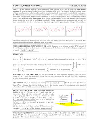
![kernel
image
domain
codomain
WHY DO WE LOOK AT THE KERNEL?
WHY DO WE LOOK AT THE IMAGE?
• It is useful to understand linear maps. To which
• A solution Ax = b can be solved if and only if b
degree are they non-invertible?
is in the image of A.
• Helpful to understand quantitatively how many
• Knowing about the kernel and the image is use-
solutions a linear equation Ax = b has. If x is
ful in the similar way that it is useful to know
a solution and y is in the kernel of A, then also
about the domain and range of a general map
A(x + y) = b, so that x + y solves the system
and to understand the graph of the map.
also.
In general, the abstraction helps to understand topics like error correcing codes (Problem 53/54 in Bretschers
book), where two matrices H, M with the property that ker(H) = im(M ) appear. The encoding x → M x is
robust in the sense that adding an error e to the result M x → M x + e can be corrected: H(M x + e) = He
allows to find e and so M x. This allows to recover x = P M x with a projection P .
PROBLEM. Find ker(A) and im(A) for the 1 × 3 matrix A = [5, 1, 4], a row vector.
ANSWER. A · x = Ax = 5x + y + 4z = 0 shows that the kernel is a plane with normal vector [5, 1, 4] through
the origin. The image is the codomain, which is R.
PROBLEM. Find ker(A) and im(A) of the linear map x → v × x, (the cross product with v.
ANSWER. The kernel consists of the line spanned by v, the image is the plane orthogonal to v.
PROBLEM. Fix a vector w in space. Find ker(A) and image im(A) of the linear map from R 6 to R3 given by
x, y → [x, v, y] = (x × y) · w.
ANSWER. The kernel consist of all (x, y) such that their cross product orthogonal to w. This means that the
plane spanned by x, y contains w.
PROBLEM Find ker(T ) and im(T ) if T is a composition of a rotation R by 90 degrees around the z-axes with
with a projection onto the x-z plane.
ANSWER. The kernel of the projection is the y axes. The x axes is rotated into the y axes and therefore the
kernel of T . The image is the x-z plane.
PROBLEM. Can the kernel of a square matrix A be trivial if A 2 = 0, where 0 is the matrix containing only 0?
ANSWER. No: if the kernel were trivial, then A were invertible and A 2 were invertible and be different from 0.
PROBLEM. Is it possible that a 3 × 3 matrix A satisfies ker(A) = R 3 without A = 0?
ANSWER. No, if A = 0, then A contains a nonzero entry and therefore, a column vector which is nonzero.
PROBLEM. What is the kernel and image of a projection onto the plane Σ : x − y + 2z = 0?
ANSWER. The kernel consists of all vectors orthogonal to Σ, the image is the plane Σ.
PROBLEM. Given two square matrices A, B and assume AB = BA. You know ker(A) and ker(B). What can
you say about ker(AB)?
ANSWER. ker(A) is contained in ker(BA). Similar ker(B) is contained in ker(AB). Because AB = BA, the
0 1
kernel of AB contains both ker(A) and ker(B). (It can be bigger: A = B = .)
0 0
A 0
PROBLEM. What is the kernel of the partitioned matrix if ker(A) and ker(B) are known?
0 B
ANSWER. The kernel consists of all vectors (x, y), where x in ker(A) and y ∈ ker(B).](https://image.slidesharecdn.com/6493617/85/Harvard_University_-_Linear_Al-22-320.jpg)


![COORDINATES Math 21b, O. Knill
| ... |
B-COORDINATES. Given a basis v1 , . . . vn , define the matrix S = v1 . . . vn . It is invertible. If
| . . . |
c1 x1
x = i ci vi , then ci are called the B-coordinates of v. We write [x]B = . . . . If x = . . . , we have
cn xn
x = S([x]B ).
B-coordinates of x are obtained by applying S −1 to the coordinates of the standard basis:
[x]B = S −1 (x) .
1 3 1 3 6
EXAMPLE. If v1 = and v2 = , then S = . A vector v = has the coordinates
2 5 2 5 9
−5 3 6 −3
S −1 v = =
2 −1 9 3
Indeed, as we can check, −3v1 + 3v2 = v.
EXAMPLE. Let V be the plane x + y − z = 1. Find a basis, in which every vector in the plane has the form
a
b . SOLUTION. Find a basis, such that two vectors v1 , v2 are in the plane and such that a third vector
0
v3 is linearly independent to the first two. Since (1, 0, 1), (0, 1, are points in the plane and (0, 0, 0) is in the
1)
1 0 1
plane, we can choose v1 = 0 v2 = 1 and v3 = 1 which is perpendicular to the plane.
1 1 −1
2 1 1
EXAMPLE. Find the coordinates of v = with respect to the basis B = {v1 = , v2 = }.
3 0 1
1 1 1 −1 −1
We have S = and S −1 = . Therefore [v]B = S −1 v = . Indeed −1v1 + 3v2 = v.
0 1 0 1 3
B-MATRIX. If B = {v1 , . . . , vn } is a basis in | ... |
Rn and T is a linear transformation on Rn , B = [T (v1 )]B . . . [T (vn )]B
then the B-matrix of T is defined as | ... |
COORDINATES HISTORY. Cartesian geometry was introduced by Fermat and Descartes (1596-1650) around
1636. It had a large influence on mathematics. Algebraic methods were introduced into geometry. The
beginning of the vector concept came only later at the beginning of the 19’th Century with the work of
Bolzano (1781-1848). The full power of coordinates becomes possible if we allow to chose our coordinate system
adapted to the situation. Descartes biography shows how far dedication to the teaching of mathematics can go ...:
(...) In 1649 Queen Christina of Sweden persuaded Descartes to go to Stockholm. However the Queen wanted to
draw tangents at 5 a.m. in the morning and Descartes broke the habit of his lifetime of getting up at 11 o’clock.
After only a few months in the cold northern climate, walking to the palace at 5 o’clock every morning, he died
of pneumonia.
Fermat Descartes Christina Bolzano](https://image.slidesharecdn.com/6493617/85/Harvard_University_-_Linear_Al-27-320.jpg)
![CREATIVITY THROUGH LAZINESS? Legend tells that Descartes (1596-1650) introduced coordinates
while lying on the bed, watching a fly (around 1630), that Archimedes (285-212 BC) discovered a method
to find the volume of bodies while relaxing in the bath and that Newton (1643-1727) discovered New-
ton’s law while lying under an apple tree. Other examples are August Kekul´’s analysis of the Benzene
e
molecular structure in a dream (a snake biting in its tail revieled the ring structure) or Steven Hawkings discovery that
black holes can radiate (while shaving). While unclear which of this is actually true, there is a pattern:
According David Perkins (at Harvard school of education): ”The Eureka effect”, many creative breakthroughs have in
common: a long search without apparent progress, a prevailing moment and break through, and finally, a
transformation and realization. A breakthrough in a lazy moment is typical - but only after long struggle
and hard work.
EXAMPLE. Let T be the reflection at the plane x + 2y + 3z = 0. Find the transformation matrix B in the
2 1 0
basis v1 = −1 v2 = 2 v3 = 3 . Because T (v1 ) = v1 = [e1 ]B , T (v2 ) = v2 = [e2 ]B , T (v3 ) = −v3 =
0 3 −2
1 0 0
−[e3 ]B , the solution is B = 0 −1 0 .
0 0 1
| ... |
SIMILARITY. The B matrix of A is B = S −1 AS, where S = v1 . . . vn . One says B is similar to A.
| ... |
EXAMPLE. If A is similar to B, then A2 +A+1 is similar to B 2 +B +1. B = S −1 AS, B 2 = S −1 B 2 S, S −1 S = 1,
S −1 (A2 + A + 1)S = B 2 + B + 1.
PROPERTIES OF SIMILARITY. A, B similar and B, C similar, then A, C are similar. If A is similar to B,
then B is similar to A.
0 1
QUIZZ: If A is a 2 × 2 matrix and let S = , What is S −1 AS?
1 0
MAIN IDEA OF CONJUGATION S. The transformation S −1 maps the coordinates from the standard basis
into the coordinates of the new basis. In order to see what a transformation A does in the new coordinates,
we map it back to the old coordinates, apply A and then map it back again to the new coordinates: B = S −1 AS.
S
v ← w = [v]B
The transformation in A↓ ↓B The transformation in
standard coordinates. S −1 B-coordinates.
Av → Bw
QUESTION. Can the matrix A which belongs to a projection from R 3 to a plane x + y + 6z = 0 be similar to
a matrix which is a rotation by 20 degrees around the z axis? No: a non-invertible A can not be similar to an
invertible B: if it were, the inverse A = SBS −1 would exist: A−1 = SB −1 S −1 .
1 −2
PROBLEM. Find a clever basis for the reflection of a light ray at the line x + 2y = 0. v 1 = , v2 = .
2 1
1 0 1 −2
SOLUTION. You can achieve B = with S = .
0 −1 2 1
1 a
PROBLEM. Are all shears A = with a = 0 similar? Yes, use a basis v1 = ae1 and v2 = e2 .
0 1
3 0 1 0 0 −1
PROBLEM. You know A = is similar to B = with S = . Find eA =
−1 2 0 −1 1 1
1/e 0
1+A+A2 +A3 /3!+.... SOLUTION. Because B k = S −1 Ak S for every k we have eA = SeB S −1 = .
e + 1/e e](https://image.slidesharecdn.com/6493617/85/Harvard_University_-_Linear_Al-28-320.jpg)
![ORTHOGONALITY Math 21b, O. Knill
ORTHOGONALITY. v and w are called orthogonal if v · w = 0.
1 6
Examples. 1) and are orthogonal in R2 . 2) v and w are both orthogonal to v × w in R3 .
2 −3
√
v is called a unit vector if ||v|| = v · v = 1. B = {v1 , . . . , vn } are called orthogonal if they are pairwise
orthogonal. They are called orthonormal if they are also unit vectors. A basis is called an orthonormal
basis if it is orthonormal. For an orthonormal basis, the matrix A ij = vi · vj is the unit matrix.
FACT. Orthogonal vectors are linearly independent and n orthogonal vectors in R n form a basis.
Proof. The dot product of a linear relation a1 v1 + . . . + an vn = 0 with vk gives ak vk · vk = ak ||vk ||2 = 0 so
that ak = 0. If we have n linear independent vectors in Rn then they automatically span the space.
ORTHOGONAL COMPLEMENT. A vector w ∈ Rn is called orthogonal to a linear space V if w is orthogonal
to every vector in v ∈ V . The orthogonal complement of a linear space V is the set W of all vectors which
are orthogonal to V . It forms a linear space because v · w 1 = 0, v · w2 = 0 implies v · (w1 + w2 ) = 0.
ORTHOGONAL PROJECTION. The orthogonal projection onto a linear space V with orthnormal basis
v1 , . . . , vn is the linear map T (x) = projV (x) = (v1 · x)v1 + . . . + (vn · x)vn The vector x − projV (x) is in the
orthogonal complement of V . (Note that vi in the projection formula are unit vectors, they have also to be
orthogonal.)
SPECIAL CASE. For an orthonormal basis vi , one can write x = (v1 · x)v1 + ... + (vn · x)vn .
PYTHAGORAS: If x and y are orthogonal, then ||x + y|| 2 = ||x||2 + ||y||2 . Proof. Expand (x + y) · (x + y).
PROJECTIONS DO NOT INCREASE LENGTH: ||projV (x)|| ≤ ||x||. Proof. Use Pythagoras: on x =
projV (x) + (x − projV (x))). If ||projV (x)|| = ||x||, then x is in V .
CAUCHY-SCHWARTZ INEQUALITY: |x · y| ≤ ||x|| ||y|| . Proof: x · y = ||x||||y|| cos(α).
If |x · y| = ||x||||y||, then x and y are parallel.
TRIANGLE INEQUALITY: ||x + y|| ≤ ||x|| + ||y||. Proof: (x + y) · (x + y) = ||x|| 2 + ||y||2 + 2x · y ≤
||x||2 + ||y||2 + 2||x||||y|| = (||x|| + ||y||)2 .
ANGLE. The angle between two vectors x, y is
x·y
α = arccos .
||x||||y||
x·y
CORRELATION. cos(α) = ||x||||y|| is called the correlation between x
and y. It is a number in [−1, 1].
EXAMPLE. The angle between two orthogonal vectors is 90 degrees or 270 degrees. If x and y represent data
x·y
showing the deviation from the mean, then ||x||||y|| is called the statistical correlation of the data.
QUESTION. Express the fact that x is in the kernel of a matrix A using orthogonality.
ANSWER: Ax = 0 means that wk · x = 0 for every row vector wk of Rn .
REMARK. We will call later the matrix AT , obtained by switching rows and columns of A the transpose of
A. You see already that the image of AT is orthogonal to the kernel of A.
1 4
2 5
QUESTION. Find a basis for the orthogonal complement of the linear space V spanned by
3 , 6 .
4 7
x
y
ANSWER: The orthogonality of
z to the two vectors means solving the linear system of equations x +
u
1 2 3 4
2y + 3z + 4w = 0, 4x + 5y + 6z + 7w = 0. An other way to solve it: the kernel of A = is the
4 5 6 7
orthogonal complement of V . This reduces the problem to an older problem.](https://image.slidesharecdn.com/6493617/85/Harvard_University_-_Linear_Al-29-320.jpg)


![ORTHOGONAL PROJECTION If v1 , . . . , vn is a basis in V which is not necessarily orthonormal, then
the orthogonal projection is x → A(AT A)−1 AT (x) where A = [v1 , . . . , vn ].
Proof. x = (AT A)−1 AT b is the least square solution of Ax = b. Therefore Ax = A(AT A)−1 AT b is the vector
in im(A) closest to b.
Special case: If w1 , . . . , wn is an orthonormal basis in V , we had seen earlier that AA T with A = [w1 , . . . , wn ]
is the orthogonal projection onto V (this was just rewriting Ax = (w 1 · x)w1 + · · · + (wn · x)wn in matrix form.)
This follows from the above formula because AT A = I in that case.
1 0
EXAMPLE Let A = 2 0 . The orthogonal projection onto V = im(A) is b → A(AT A)−1 AT b. We have
0 1
1/5 2/5 0
5 0
AT A = and A(AT A)−1 AT = 2/5 4/5 0 .
2 1
0 0 1
0 2/5 √
For example, the projection of b = 1 is x∗ = 4/5 and the distance to b is 1/ 5. The point x∗ is the
0 0
point on V which is closest to b.
Remember the formula for the distance of b to a plane V with normal vector n? It was d = |n · b|/||n||. In our
√
case, we can take n = [−2, 1, 0] this formula gives the distance 1/ 5. Let’s check: the distance of x∗ and b is
√
||(2/5, −1/5, 0)|| = 1/ 5.
1
2
EXAMPLE. Let A =
0 . Problem: find the matrix of the orthogonal projection onto the image of A.
1
The image of A is a one-dimensional line spanned by the vector v = (1, 2, 0, 1). We calculate A T A = 6. Then
1 1 2 0 1
2 2 4 0 2
A(AT A)−1 AT =
0 1 2 0 1 /6 = 0 0 0 0 /6
1 1 2 0 1
DATA FIT. Find a quadratic polynomial p(t) = at2 + bt + c which best fits the four data points
(−1, 8), (0, 8), (1, 4), (2, 16).
T
1 −1 1 8 Software packages like Mathematica have already
0 0 1 8 built in the facility to fit numerical data:
A =
1 1 1 b = 4 .
AT A =
4 2 1 16
18 8 6 3
8 6 2 and x∗ = (AT A)−1 AT b = −1 .
6 2 4 5
The series expansion of f showed that indeed, f (t) = 5 − t + 3t 2 is indeed best quadratic fit. Actually,
Mathematica does the same to find the fit then what we do: ”Solving” an inconsistent system of linear
equations as best as possible.
PROBLEM: Prove im(A) = im(AAT ).
SOLUTION. The image of AAT is contained in the image of A because we can write v = AA T x as v = Ay with
y = AT x. On the other hand, if v is in the image of A, then v = Ax. If x = y + z, where y in the kernel of
A and z orthogonal to the kernel of A, then Ax = Az. Because z is orthogonal to the kernel of A, it is in the
image of AT . Therefore, z = AT u and v = Az = AAT u is in the image of AAT .](https://image.slidesharecdn.com/6493617/85/Harvard_University_-_Linear_Al-36-320.jpg)


![PARTITIONED MATRICES.
TRIANGULAR AND DIAGONAL MATRICES.
The determinant of a partitioned matrix
The determinant of a diagonal or triangular ma- A 0
trix is the product of its diagonal elements.
is the product det(A)det(B).
0 B
1 0 0 0
4 5 0 0 3 4 0 0
Example: det(
2 3 4 0 ) = 20.
1 2 0 0
Example det(
0 0 4 −2 ) = 2 · 12 = 24.
1 1 2 1
0 0 2 2
LINEARITY OF THE DETERMINANT. If the columns of A and B are the same except for the i’th column,
det([v1 , ..., v, ...vn ]] + det([v1 , ..., w, ...vn ]] = det([v1 , ..., v + w, ...vn ]] .
In general, one has
det([v1 , ..., kv, ...vn ]] = k det([v1 , ..., v, ...vn ]] .
The same holds for rows. These identities follow directly from the original definition of the determimant.
det(AB) = det(A)det(B) . det(SAS −1 ) = det(A) . de
PROPERTIES OF DETERMINANTS.
det(AT ) = det(A) det(−
det(A−1 ) = det(A)−1
If B is obtained from A by switching two rows, then det(B) = −det(A). If B is obtained by adding an other
row to a given row, then this does not change the value of the determinant.
PROOF OF det(AB) = det(A)det(B), one brings the n × n matrix [A|AB] into row reduced echelon form.
Similar than the augmented matrix [A|b] was brought into the form [1|A −1 b], we end up with [1|A−1 AB] = [1|B].
By looking at the n × n matrix to the left during Gauss-Jordan elimination, the determinant has changed by a
factor det(A). We end up with a matrix B which has determinant det(B). Therefore, det(AB) = det(A)det(B).
PROOF OF det(AT ) = det(A). The transpose of a pattern is a pattern with the same signature.
PROBLEM. Find the determi-
1 2 4 5
0 0 0 2 0 7 2 9
1 2 4 5 SOLUTION. Three row transpositions give B =
0 0 6 4 a ma-
nant of A =
0 7 2
.
9 0 0 0 2
0 0 6 4 trix which has determinant 84. Therefore det(A) = (−1) 3 det(B) = −84.
1 2
PROBLEM. Determine det(A100 ), where A is the matrix .
3 16
SOLUTION. det(A) = 10, det(A100 ) = (det(A))100 = 10100 = 1 · gogool. This name as well as the gogoolplex =
100 51
1010 are official. They are huge numbers: the mass of the universe for example is 10 52 kg and 1/1010 is the
chance to find yourself on Mars by quantum fluctuations. (R.E. Crandall, Scient. Amer., Feb. 1997).
ROW REDUCED ECHELON FORM. Determining rref(A) also determines det(A).
If A is a matrix and αi are the factors which are used to scale different rows and s is the number of times, two
rows are switched, then det(A) = (−1)s α1 · · · αn det(rref(A)) .
INVERTIBILITY. Because of the last formula: A n × n matrix A is invertible if and only if det(A) = 0.
THE LAPLACE EXPANSION.
In order to calculate by hand the determinant of n × n matrices A = a ij for n > 3, the following expansion
is useful. Choose a column i. For each entry aji in that column, take the (n − 1) × (n − 1) matrix Aij called
minor which does not contain the i’th column and j’th row. Then
n
det(A) = (−1)i+1 ai1 det(Ai1 ) + · · · + (−1)i+n ain det(Ain ) = j=1 (−1)
i+j
aij det(Aij )
ORTHOGONAL MATRICES. Because QT Q = 1, we have det(Q)2 = 1 and so |det(Q)| = 1 Rotations have
determinant 1, reflections have determinant −1.
QR DECOMPOSITION. If A = QR, then det(A) = det(Q)det(R). The determinant of Q is ±1, the determinant
of R is the product of the diagonal elements of R.](https://image.slidesharecdn.com/6493617/85/Harvard_University_-_Linear_Al-40-320.jpg)
![DETERMINANTS II, Math 21b, O.Knill
DETERMINANT AND VOLUME. If A is a n × n matrix, then |det(A)| is the volume of the n-dimensional
parallelepiped En spanned by the n column vectors vj of A.
Proof. Use the QR decomposition A = QR, where Q is orthogonal and R is
upper triangular. From QQT = 1, we get 1 = det(Q)det(QT ) = det(Q)2 see that
|det(Q)| = 1. Therefore, det(A) = ±det(R). The determinant of R is the product
of the ||ui || = ||vi − projVj−1 vi || which was the distance from vi to Vj−1 . The
volume vol(Ej ) of a j-dimensional parallelepiped Ej with base Ej−1 in Vj−1 and
height ||ui || is vol(Ej−1 )||uj ||. Inductively vol(Ej ) = ||uj ||vol(Ej−1 ) and therefore
n
vol(En ) = j=1 ||uj || = det(R).
The volume of a k dimensional parallelepiped defined by the vectors v 1 , . . . , vk is det(AT A).
k
Proof. QT Q = In gives AT A = (QR)T (QR) = RT QT QR = RT R. So, det(RT R) = det(R)2 = ( j=1 ||uj ||)2 .
(Note that A is a n × k matrix and that AT A = RT R and R are k × k matrices.)
ORIENTATION. Determinants allow to define the orientation of n vectors in n-dimensional space. This is
”handy” because there is no ”right hand rule” in hyperspace... To do so, define the matrix A with column
vectors vj and define the orientation as the sign of det(A). In three dimensions, this agrees with the right hand
rule: if v1 is the thumb, v2 is the pointing finger and v3 is the middle finger, then their orientation is positive.
x i det(A) =
CRAMER’S RULE. This is an explicit formula for the solution of Ax = b. If Ai
denotes the matrix, where the column vi of A is replaced by b, then
det b xi = det(Ai )/det(A)
Proof. det(Ai ) = det([v1 , . . . , b, . . . , vn ] = det([v1 , . . . , (Ax), . . . , vn ] =
det([v1 , . . . , i xi vi , . . . , vn ] = xi det([v1 , . . . , vi , . . . , vn ]) = xi det(A)
i
5 3
EXAMPLE. Solve the system 5x+3y = 8, 8x+5y = 2 using Cramers rule. This linear system with A =
8 5
8 8 3 5 8
and b = . We get x = det = 34y = det = −54.
2 2 5 8 2
GABRIEL CRAMER. (1704-1752), born in Geneva, Switzerland, he worked on geometry
and analysis. Cramer used the rule named after him in a book ”Introduction a l’analyse
`
des lignes courbes alg´braique”, where he solved like this a system of equations with 5
e
unknowns. According to a short biography of Cramer by J.J O’Connor and E F Robertson,
the rule had however been used already before by other mathematicians. Solving systems
with Cramers formulas is slower than by Gaussian elimination. The rule is still important.
For example, if A or b depends on a parameter t, and we want to see how x depends on
the parameter t one can find explicit formulas for (d/dt)x i (t).
THE INVERSE OF A MATRIX. Because the columns of A−1 are solutions of Ax = ei , where ej are basis
vectors, Cramers rule together with the Laplace expansion gives the formula:
[A−1 ]ij = (−1)i+j det(Aji )/det(A)
Bij = (−1)i+j det(Aji ) is called the classical adjoint of A. Note the change ij → ji. Don’t confuse the
classical adjoint with the transpose AT which is sometimes also called the adjoint.](https://image.slidesharecdn.com/6493617/85/Harvard_University_-_Linear_Al-41-320.jpg)

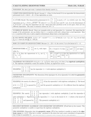
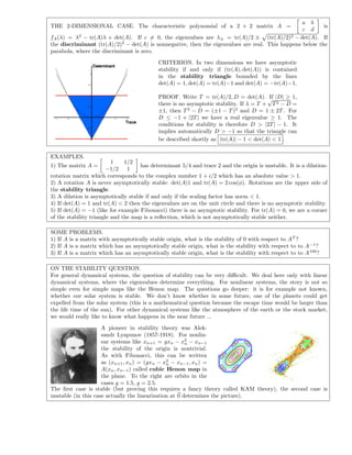
![COMPUTING EIGENVALUES Math 21b, O.Knill
THE TRACE. The trace of a matrix A is the sum of its diagonal elements.
1 2 3
EXAMPLES. The trace of A = 3 4 5 is 1 + 4 + 8 = 13. The trace of a skew symmetric matrix A is zero
6 7 8
because there are zeros in the diagonal. The trace of I n is n.
CHARACTERISTIC POLYNOMIAL. The polynomial fA (λ) = det(λIn − A) is called the characteristic
polynomial of A.
EXAMPLE. The characteristic polynomial of A above is x 3 − 13x2 + 15x.
The eigenvalues of A are the roots of the characteristic polynomial f A (λ).
Proof. If λ is an eigenvalue of A with eigenfunction v, then A − λ has v in the kernel and A − λ is not invertible
so that fA (λ) = det(λ − A) = 0.
The polynomial has the form
fA (λ) = λn − tr(A)λn−1 + · · · + (−1)n det(A)
a b
THE 2x2 CASE. The characteristic polynomial of A = is fA (λ) = λ2 − (a + d)/2λ + (ad − bc). The
c d
eigenvalues are λ± = T /2 ± (T /2)2 − D, where T is the trace and D is the determinant. In order that this
is real, we must have (T /2)2 ≥ D. Away from that parabola, there are two different eigenvalues. The map A
contracts volume for |D| < 1.
1 2
EXAMPLE. The characteristic polynomial of A = is λ2 − 3λ + 2 which has the roots 1, 2: pA (λ) =
0 2
(λ − 1)(λ − 2).
THE FIBONNACCI RABBITS. The Fibonacci’s recursion un+1 = un + un−1 defines the growth of the rabbit
un+1 un 1 1
population. We have seen that it can be rewritten as =A with A = . The roots
un un−1 1 0
√ √
of the characteristic polynomial pA (x) = λ2 − λ − 1. are ( 5 + 1)/2, ( 5 − 1)/2.
ALGEBRAIC MULTIPLICITY. If fA (λ) = (λ − λ0 )k g(λ), where g(λ0 ) = 0 then λ is said to be an eigenvalue
of algebraic multiplicity k.
1 1 1
EXAMPLE: 0 1 1 has the eigenvalue λ = 1 with algebraic multiplicity 2 and the eigenvalue λ = 2 with
0 0 2
algebraic multiplicity 1.
HOW TO COMPUTE EIGENVECTORS? Because (λ − A)v = 0, the vector v is in the kernel of λ − A. We
know how to compute the kernel.
λ± − 1 −1 √
EXAMPLE FIBONNACCI. The kernel of λI2 − A = is spanned by v+ = (1 + 5)/2, 1
−1 λ±
√
and v− = (1 − 5)/2, 1 . They form a basis B.
1 1 √
SOLUTION OF FIBONNACCI. To obtain a formula for An v with v = , we form [v]B = / 5.
0 −1
un+1 √ √ √ √ √ √
Now, = An v = An (v+ / 5 − v− / 5) = An v+ / 5 − An (v− / 5 = λn v+ / 5 + λn v+ / 5. We see that
+ −
un
√ √ √
un = [( 1+2 5 )n + ( 1−2 5 )n ]/ 5.
ROOTS OF POLYNOMIALS.
For polynomials of degree 3 and 4 there exist explicit formulas in terms of radicals. As Galois (1811-1832) and
Abel (1802-1829) have shown, it is not possible for equations of degree 5 or higher. Still, one can compute the
roots numerically.](https://image.slidesharecdn.com/6493617/85/Harvard_University_-_Linear_Al-43-320.jpg)
![REAL SOLUTIONS. A (2n + 1) × (2n + 1) matrix A always has a real eigenvalue
because the characteristic polynomial p(x) = x 5 + ... + det(A) has the property
that p(x) goes to ±∞ for x → ±∞. Because there exist values a, b for which
p(a) < 0 and p(b) > 0, by the intermediate value theorem, there exists a real x
with p(x) = 0. Application: A rotation in 11 dimensional space has all eigenvalues
|λ| = 1. The real eigenvalue must have an eigenvalue 1 or −1.
EIGENVALUES OF TRANSPOSE. We know (see homework) that the characteristic polynomials of A and A T
agree. Therefore A and AT have the same eigenvalues.
APPLICATION: MARKOV MATRICES. A matrix A for which each column sums up to 1 is called a Markov
1
1
matrix. The transpose of a Markov matrix has the eigenvector
. . . with eigenvalue 1. Therefore:
1
A Markov matrix has an eigenvector v to the eigenvalue 1.
This vector v defines an equilibrium point of the Markov process.
1/3 1/2
EXAMPLE. If A = . Then [3/7, 4/7] is the equilibrium eigenvector to the eigenvalue 1.
2/3 1/2
BRETSCHERS HOMETOWN. Problem 28 in the
book deals with a Markov problem in Andelfingen
the hometown of Bretscher, where people shop in two
shops. (Andelfingen is a beautiful village at the Thur
river in the middle of a ”wine country”). Initially
all shop in shop W . After a new shop opens, every
week 20 percent switch to the other shop M . Missing
something at the new place, every week, 10 percent
switch back. This leads to a Markov matrix A =
8/10 1/10
. After some time, things will settle
2/10 9/10
down and we will have certain percentage shopping
in W and other percentage shopping in M . This is
the equilibrium.
.
MARKOV PROCESS IN PROBABILITY. Assume we have a graph like a
network and at each node i, the probability to go from i to j in the next step
is [A]ij , where Aij is a Markov matrix. We know from the above result that
there is an eigenvector p which satisfies Ap = p. It can be normalized that
i pi = 1. The interpretation is that p i is the probability that the walker is on
A C
the node p. For example, on a triangle, we can have the probabilities: P (A →
B) = 1/2, P (A → C) = 1/4, P (A → A) = 1/4, P (B → A) = 1/3, P (B → B) =
1/6, P (B → C) = 1/2, P (C → A) = 1/2, P (C → B) = 1/3, P (C → C) = 1/6.
The corresponding matrix is
B
1/4 1/3 1/2
A = 1/2 1/6 1/3 .
1/4 1/2 1/6
In this case, the eigenvector to the eigenvalue 1 is p =
[38/107, 36/107, 33/107]T .](https://image.slidesharecdn.com/6493617/85/Harvard_University_-_Linear_Al-44-320.jpg)
![DIAGONALIZATION Math 21b, O.Knill
SUMMARY. A n × n matrix, Av = λv with eigenvalue λ and eigenvector v. The eigenvalues are the roots of
the characteristic polynomial fA (λ) = det(λ − A) = λn − tr(A)λn−1 + ... + (−1)n det(A). The eigenvectors to
the eigenvalue λ are in ker(λ − A). The number of times, an eigenvalue λ occurs in the full list of n roots of
fA (λ) is called algebraic multiplicity. It is bigger or equal than the geometric multiplicity: dim(ker(λ − A).
a b
EXAMPLE. The eigenvalues of are λ± = T /2 + T 2 /4 − D, where T = a + d is the trace and
c d
λ± − d
D = ad − bc is the determinant of A. If c = 0, the eigenvectors are v ± = if c = 0, then a, d are
c
a −b
eigenvalues to the eigenvectors and . If a = d, then the second eigenvector is parallel to the
0 a−d
first and the geometric multiplicity of the eigenvalue a = d is 1.
EIGENBASIS. If A has n different eigenvalues, then A has an eigenbasis, consisting of eigenvectors of A.
DIAGONALIZATION. How does the matrix A look in an eigenbasis? If S is the matrix with the eigenvectors as
columns, then we know B = S −1 AS . We have Sei = vi and ASei = λi vi we know S −1 ASei = λi ei . Therefore,
B is diagonal with diagonal entries λi .
2 3 √ √
EXAMPLE. A = 3 with eigenvector v1 = [ 3, 1] and the eigenvalues
has the eigenvalues λ1 = 2 +
1 2
√ √
√ √ 3 − 3
λ2 = 2 − 3 with eigenvector v2 = [− 3, 1]. Form S = and check S −1 AS = D is diagonal.
1 1
APPLICATION: FUNCTIONAL CALCULUS. Let A be the matrix in the above example. What is A 100 +
A37 − 1? The trick is to diagonalize A: B = S −1 AS, then B k = S −1 Ak S and We can compute A100 + A37 − 1 =
S(B 100 + B 37 − 1)S −1 .
APPLICATION: SOLVING LINEAR SYSTEMS. x(t+1) = Ax(t) has the solution x(n) = A n x(0). To compute
An , we diagonalize A and get x(n) = SB n S −1 x(0). This is an explicit formula.
SIMILAR MATRICES HAVE THE SAME EIGENVALUES.
One can see this in two ways:
1) If B = S −1 AS and v is an eigenvector of B to the eigenvalue λ, then Sv is an eigenvector of A to the
eigenvalue λ.
2) From det(S −1 AS) = det(A), we know that the characteristic polynomials f B (λ) = det(λ − B) = det(λ −
S −1 AS) = det(S −1 (λ − AS) = det((λ − A) = fA (λ) are the same.
CONSEQUENCES.
1) Because the characteristic polynomials of similar matrices agree, the trace tr(A) of similar matrices agrees.
2) The trace is the sum of the eigenvalues of A. (Compare the trace of A with the trace of the diagonalize
matrix.)
THE CAYLEY HAMILTON THEOREM. If A is diagonalizable, then fA (A) = 0.
PROOF. The DIAGONALIZATION B = S −1 AS has the eigenvalues in the diagonal. So fA (B), which
contains fA (λi ) in the diagonal is zero. From fA (B) = 0 we get SfA (B)S −1 = fA (A) = 0.
By the way: the theorem holds for all matrices: the coefficients of a general matrix can be changed a tiny bit so that all eigenvalues are different. For any such
perturbations one has fA (A) = 0. Because the coefficients of fA (A) depend continuously on A, they are zero 0 in general.
CRITERIA FOR SIMILARITY.
• If A and B have the same characteristic polynomial and diagonalizable, then they are similar.
• If A and B have a different determinant or trace, they are not similar.
• If A has an eigenvalue which is not an eigenvalue of B, then they are not similar.](https://image.slidesharecdn.com/6493617/85/Harvard_University_-_Linear_Al-47-320.jpg)
![WHY DO WE WANT TO DIAGONALIZE?
1) FUNCTIONAL CALCULUS. If p(x) = 1 + x + x2 + x3 /3! + x4 /4! be a polynomial and A is a matrix, then
p(A) = 1 + A + A2 /2! + A3 /3! + A4 /4! is a matrix. If B = S −1 AS is diagonal with diagonal entries λi , then
p(B) is diagonal with diagonal entries p(λi ). And p(A) = S p(B)S −1 . This speeds up the calculation because
matrix multiplication costs much. The matrix p(A) can be written down with three matrix multiplications,
because p(B) is diagonal.
˙
2) SOLVING LINEAR DIFFERENTIAL EQUATIONS. A differential equation v = Av is solved by
At At 2 2 3 3
v(t) = e v(0), where e = 1 + At + A t /2! + A t /3!...)x(0). (Differentiate this sum with respect to t
to get AeAt v(0) = Ax(t).) If we write this in an eigenbasis of A, then y(t) = e Bt y(0) with the diagonal
λ1 0 . . . 0
matrix B = 0 λ2 . . . 0 . In other words, we have then explicit solutions y j (t) = eλj t yj (0). Linear
0 0 . . . λn
differential equations later in this course. It is important motivation.
3) STOCHASTIC DYNAMICS (i.e MARKOV PROCESSES). Complicated systems can be modeled by putting
probabilities on each possible event and computing the probabilities that an event switches to any other event.
This defines a transition matrix. Such a matrix always has an eigenvalue 1. The corresponding eigenvector
is the stable probability distribution on the states. If we want to understand, how fast things settle to this
equilibrium, we need to know the other eigenvalues and eigenvectors.
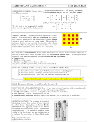
MOLECULAR VIBRATIONS. While quantum mechanics describes the motion of atoms in molecules, the
vibrations can be described classically, when treating the atoms as ”balls” connected with springs. Such ap-
proximations are necessary when dealing with large atoms, where quantum mechanical computations would be
too costly. Examples of simple molecules are white phosphorus P 4 , which has tetrahedronal shape or methan
CH4 the simplest organic compound or freon, CF2 Cl2 which is used in refrigerants. Caffeine or aspirin form
more complicated molecules.
Freon CF2 Cl2 Caffeine C8 H10 N4 O2 Aspirin C9 H8 O4
WHITE PHOSPHORUS VIBRATIONS. (Differential equations appear later, the context is motivation at this
stage). Let x1 , x2 , x3 , x4 be the positions of the four phosphorus atoms (each of them is a 3-vector). The inter-
atomar forces bonding the atoms is modeled by springs. The first atom feels a force x 2 − x1 + x3 − x1 + x4 − x1
and is accelerated in the same amount. Let’s just chose units so that the force is equal to the acceleration. Then
x1
¨ = (x2 − x1 ) + (x3 − x1 ) + (x4 − x1 )
which has the form x =
¨
x2
¨ = (x3 − x2 ) + (x4 − x2 ) + (x1 − x2 )
Ax, where the 4 × 4 ma-
x3
¨ = (x4 − x3 ) + (x1 − x3 ) + (x2 − x3 ) trix
x4
¨ = (x1 − x4 ) + (x2 − x4 ) + (x3 − x4 )
−3 1 1 1 1 −1 −1 −1
1 −3 1 1 1 0 0 1
A= v1 =
1 , v2 = 0
, v3 =
1 , v4 = 0
1 1 −3 1
1 1 1 −3 1 1 0 0
are the eigenvectors to the eigenvalues λ1 = 0, λ2 = −4, λ3 = −4, λ3 = −4. With S = [v1 v2 v3 v4 ],
the matrix B = S −1 BS is diagonal with entries 0, −4, −4, −4. The coordinates y i = Sxi satisfy
y1 = 0, y2 = −4y2 , y3 = −4y3 , y4 = −4y4 which we can solve y0 which is the center of mass satisfies
¨ ¨ ¨ ¨
y0 = a + bt (move molecule with constant speed). The motions y i = ai cos(2t) + bi sin(2t) of the other
eigenvectors are oscillations, called normal modes. The general motion of the molecule is a superposition of
these modes.](https://image.slidesharecdn.com/6493617/85/Harvard_University_-_Linear_Al-48-320.jpg)

![Gauss published the first correct proof of the fundamental theorem of algebra in his doctoral thesis, but still
claimed in 1825 that the true metaphysics of the square root of −1 is elusive as late as 1825. By 1831
Gauss overcame his uncertainty about complex numbers and published his work on the geometric representation
of complex numbers as points in the plane. In 1797, a Norwegian Caspar Wessel (1745-1818) and in 1806 a
Swiss clerk named Jean Robert Argand (1768-1822) (who stated the theorem the first time for polynomials with
complex coefficients) did similar work. But these efforts went unnoticed. William Rowan Hamilton (1805-1865)
(who would also discover the quaternions while walking over a bridge) expressed in 1833 complex numbers as
vectors.
Complex numbers continued to develop to complex function theory or chaos theory, a branch of dynamical
systems theory. Complex numbers are helpful in geometry in number theory or in quantum mechanics. Once
believed fictitious they are now most ”natural numbers” and the ”natural numbers” themselves are in fact the
√
most ”complex”. A philospher who asks ”does −1 really exist?” might be shown the representation of x + iy
x −y
as . When adding or multiplying such dilation-rotation matrices, they behave like complex numbers:
y x
0 −1
for example plays the role of i.
1 0
FUNDAMENTAL THEOREM OF ALGEBRA. (Gauss 1799) A polynomial of degree n has exactly n roots.
CONSEQUENCE: A n × n MATRIX HAS n EIGENVALUES. The characteristic polynomial f A (λ) = λn +
an−1 λn−1 + . . . + a1 λ + a0 satisfies fA (λ) = (λ − λ1 ) . . . (λ − λn ), where λi are the roots of f .
TRACE AND DETERMINANT. Comparing fA (λ) = (λ − λn ) . . . (λ − λn ) with λn − tr(A) + .. + (−1)n det(A)
gives tr(A) = λ1 + · · · + λn , det(A) = λ1 · · · λn .
COMPLEX FUNCTIONS. The characteristic polynomial
is an example of a function f from C to C. The graph of
this function would live in C × C which corresponds to a
l l
four dimensional real space. One can visualize the function
however with the real-valued function z → |f (z)|. The
figure to the left shows the contour lines of such a function
z → |f (z)|, where f is a polynomial.
ITERATION OF POLYNOMIALS. A topic which
is off this course (it would be a course by itself)
is the iteration of polynomials like fc (z) = z 2 + c.
The set of parameter values c for which the iterates
2 n
fc (0), fc (0) = fc (fc (0)), . . . , fc (0) stay bounded is called
the Mandelbrot set. It is the fractal black region in the
picture to the left. The now already dusty object appears
everywhere, from photoshop plugins to decorations. In
Mathematica, you can compute the set very quickly (see
http://www.math.harvard.edu/computing/math/mandelbrot.m).
COMPLEX √ NUMBERS IN MATHEMATICA OR MAPLE. In both computer algebra systems, the letter I is
used for i = −1. In Maple, you can ask log(1 + I), in Mathematica, this would be Log[1 + I]. Eigenvalues or
eigenvectors of a matrix will in general involve complex numbers. For example, in Mathematica, Eigenvalues[A]
gives the eigenvalues of a matrix A and Eigensystem[A] gives the eigenvalues and the corresponding eigenvectors.
cos(φ) sin(φ)
EIGENVALUES AND EIGENVECTORS OF A ROTATION. The rotation matrix A =
− sin(φ) cos(φ)
has the characteristic polynomial λ2 − 2 cos(φ) + 1. The eigenvalues are cos(φ) ± cos2 (φ) − 1 = cos(φ) ±
−i
i sin(φ) = exp(±iφ). The eigenvector to λ1 = exp(iφ) is v1 = and the eigenvector to the eigenvector
1
i
λ2 = exp(−iφ) is v2 = .
1](https://image.slidesharecdn.com/6493617/85/Harvard_University_-_Linear_Al-50-320.jpg)

![SYMMETRIC MATRICES Math 21b, O. Knill
SYMMETRIC MATRICES. A matrix A with real entries is symmetric, if AT = A.
1 2 1 1
EXAMPLES. A = is symmetric, A = is not symmetric.
2 3 0 3
EIGENVALUES OF SYMMETRIC MATRICES. Symmetric matrices A have real eigenvalues.
PROOF. The dot product is extend to complex vectors as (v, w) = i v i wi . For real vectors it satisfies
(v, w) = v · w and has the property (Av, w) = (v, AT w) for real matrices A and (λv, w) = λ(v, w) as well as
(v, λw) = λ(v, w). Now λ(v, v) = (λv, v) = (Av, v) = (v, AT v) = (v, Av) = (v, λv) = λ(v, v) shows that λ = λ
because (v, v) = 0 for v = 0.
p −q
EXAMPLE. A = has eigenvalues p + iq which are real if and only if q = 0.
q p
EIGENVECTORS OF SYMMETRIC MATRICES. Symmetric matrices have an orthonormal eigenbasis
PROOF. If Av = λv and Aw = µw. The relation λ(v, w) = (λv, w) = (Av, w) = (v, A T w) = (v, Aw) =
(v, µw) = µ(v, w) is only possible if (v, w) = 0 if λ = µ.
WHY ARE SYMMETRIC MATRICES IMPORTANT? In applications, matrices are often symmetric. For ex-
ample in geometry as generalized dot products v·Av, or in statistics as correlation matrices Cov[X k , Xl ]
or in quantum mechanics as observables or in neural networks as learning maps x → sign(W x) or in graph
theory as adjacency matrices etc. etc. Symmetric matrices play the same role as real numbers do among the
complex numbers. Their eigenvalues often have physical or geometrical interpretations. One can also calculate
with symmetric matrices like with numbers: for example, we can solve B 2 = A for B if A is symmetric matrix
0 1
and B is square root of A.) This is not possible in general: try to find a matrix B such that B 2 = ...
0 0
RECALL. We have seen when an eigenbasis exists, a matrix A can be transformed to a diagonal matrix
B = S −1 AS, where S = [v1 , ..., vn ]. The matrices A and B are similar. B is called the diagonalization of
A. Similar matrices have the same characteristic polynomial det(B − λ) = det(S −1 (A − λ)S) = det(A − λ)
and have therefore the same determinant, trace and eigenvalues. Physicists call the set of eigenvalues also the
spectrum. They say that these matrices are isospectral. The spectrum is what you ”see” (etymologically
the name origins from the fact that in quantum mechanics the spectrum of radiation can be associated with
eigenvalues of matrices.)
SPECTRAL THEOREM. Symmetric matrices A can be diagonalized B = S −1 AS with an orthogonal S.
PROOF. If all eigenvalues are different, there is an eigenbasis and diagonalization is possible. The eigenvectors
are all orthogonal and B = S −1 AS is diagonal containing the eigenvalues. In general, we can change the matrix
A to A = A + (C − A)t where C is a matrix with pairwise different eigenvalues. Then the eigenvalues are
different for all except finitely many t. The orthogonal matrices St converges for t → 0 to an orthogonal matrix
S and S diagonalizes A.
WAIT A SECOND ... Why could we not perturb a general matrix At to have disjoint eigenvalues and At could
−1
be diagonalized: St At St = Bt ? The problem is that St might become singular for t → 0. See problem 5) first
practice exam.
a b 1 √
EXAMPLE 1. The matrix A = has the eigenvalues a + b, a − b and the eigenvectors v1 = / 2
b a 1
−1 √
and v2 = / 2. They are orthogonal. The orthogonal matrix S = v1 v2 diagonalized A.
1](https://image.slidesharecdn.com/6493617/85/Harvard_University_-_Linear_Al-53-320.jpg)
![
1 1 1
EXAMPLE 2. The 3 × 3 matrix A = 1 1 1 has 2 eigenvalues 0 to the eigenvectors 1 −1 0 ,
1 1 1
1 0 −1 and one eigenvalue 3 to the eigenvector 1 1 1 . All these vectors can be made orthogonal
and a diagonalization is possible even so the eigenvalues have multiplicities.
SQUARE ROOT OF A MATRIX. How do we find a square root of a given symmetric matrix? Because
S −1 AS = B is diagonal and we know how to take a square root of the diagonal matrix B, we can form
√ √ √
C = S BS −1 which satisfies C 2 = S BS −1 S BS −1 = SBS −1 = A.
RAYLEIGH FORMULA. We write also (v, w) = v · w. If v(t) is an eigenvector of length 1 to the eigenvalue λ(t)
of a symmetric matrix A(t) which depends on t, differentiation of (A(t) − λ(t))v(t) = 0 with respect to t gives
(A −λ )v +(A−λ)v = 0. The symmetry of A−λ implies 0 = (v, (A −λ )v)+(v, (A−λ)v ) = (v, (A −λ )v). We
see that the Rayleigh quotient λ = (A v, v) is a polynomial in t if A(t) only involves terms t, t2 , . . . , tm . The
1 t2
formula shows how λ(t) changes, when t varies. For example, A(t) = has for t = 2 the eigenvector
t2 1
√ 0 4
v = [1, 1]/ 2 to the eigenvalue λ = 5. The formula tells that λ (2) = (A (2)v, v) = ( v, v) = 4. Indeed,
4 0
λ(t) = 1 + t2 has at t = 2 the derivative 2t = 4.
EXHIBITION. ”Where do symmetric matrices occur?” Some informal motivation:
I) PHYSICS: In quantum mechanics a system is described with a vector v(t) which depends on time t. The
evolution is given by the Schroedinger equation v = i¯ Lv, where L is a symmetric matrix and h is a small
˙ h ¯
number called the Planck constant. As for any linear differential equation, one has v(t) = e i¯ Lt v(0). If v(0) is
h
an eigenvector to the eigenvalue λ, then v(t) = eit¯ λ v(0). Physical observables are given by symmetric matrices
h
too. The matrix L represents the energy. Given v(t), the value of the observable A(t) is v(t) · Av(t). For
example, if v is an eigenvector to an eigenvalue λ of the energy matrix L, then the energy of v(t) is λ.
This is called the Heisenberg picture. In order that v · A(t)v =
v(t) · Av(t) = S(t)v · AS(t)v we have A(t) = S(T )∗ AS(t), where
S ∗ = S T is the correct generalization of the adjoint to complex
matrices. S(t) satisfies S(t)∗ S(t) = 1 which is called unitary
and the complex analogue of orthogonal. The matrix A(t) =
S(t)∗ AS(t) has the same eigenvalues as A and is similar to A.
II) CHEMISTRY. The adjacency matrix A of a graph with n vertices determines the graph: one has A ij = 1
if the two vertices i, j are connected and zero otherwise. The matrix A is symmetric. The eigenvalues λ j are
real and can be used to analyze the graph. One interesting question is to what extent the eigenvalues determine
the graph.
In chemistry, one is interested in such problems because it allows to make rough computations of the electron
density distribution of molecules. In this so called H¨ ckel theory, the molecule is represented as a graph. The
u
eigenvalues λj of that graph approximate the energies an electron on the molecule. The eigenvectors describe
the electron density distribution.
This matrix A has the eigenvalue 0 with
0 1 1 1 1 multiplicity 3 (ker(A) is obtained im-
The Freon molecule for 1 0 0 0 0
mediately from the fact that 4 rows are
example has 5 atoms. The 1 0 0 0 0 . the same) and the eigenvalues 2, −2.
adjacency matrix is 1 0 0 0 0
The eigenvector to the eigenvalue ±2 is
1 0 0 0 0 T
±2 1 1 1 1 .
III) STATISTICS. If we have a random vector X = [X1 , · · · , Xn ] and E[Xk ] denotes the expected value of
Xk , then [A]kl = E[(Xk − E[Xk ])(Xl − E[Xl ])] = E[Xk Xl ] − E[Xk ]E[Xl ] is called the covariance matrix of
the random vector X. It is a symmetric n × n matrix. Diagonalizing this matrix B = S −1 AS produces new
random variables which are uncorrelated.
For example, if X is is the sum of two dice and Y is the value of the second dice then E[X] = [(1 + 1) +
(1 + 2) + ... + (6 + 6)]/36 = 7, you throw in average a sum of 7 and E[Y ] = (1 + 2 + ... + 6)/6 = 7/2. The
matrix entry A11 = E[X 2 ] − E[X]2 = [(1 + 1) + (1 + 2) + ... + (6 + 6)]/36 − 72 = 35/6 known as the variance
of X, and A22 = E[Y 2 ] − E[Y ]2 = (12 + 22 + ... + 62 )/6 − (7/2)2 = 35/12 known as the variance of Y and
35/6 35/12
A12 = E[XY ] − E[X]E[Y ] = 35/12. The covariance matrix is the symmetric matrix A = .
35/12 35/12](https://image.slidesharecdn.com/6493617/85/Harvard_University_-_Linear_Al-54-320.jpg)

![1
1 1 1
0.5
0.5 0.5 0.5
-1 -0.5 0.5 1 -1 -0.5 0.5 1 -1 -0.5 0.5 1 -1 -0.5 0.5 1
-0.5 -0.5 -0.5
-0.5
-1 -1 -1
-1
UNDERSTANDING A DIFFERENTIAL EQUATION. The closed form solution like x(t) = e At x(0) for x = ˙
Ax is actually quite useless. One wants to understand the solution quantitatively. Questions one wants to
answer are: what happens in the long term? Is the origin stable, are there periodic solutions. Can one
decompose the system into simpler subsystems? We will see that diagonalisation allows to understand the
system: by decomposing it into one-dimensional linear systems, which can be analyzed seperately. In general,
”understanding” can mean different things:
Plotting phase portraits. Finding special closed form solutions x(t).
Computing solutions numerically and esti- Finding a power series x(t) = n an tn in t.
mate the error. Finding quantities which are unchanged along
Finding special solutions. the flow (called ”Integrals”).
Predicting the shape of some orbits. Finding quantities which increase along the
Finding regions which are invariant. flow (called ”Lyapunov functions”).
LINEAR STABILITY. A linear dynamical system x = Ax with diagonalizable A is linearly stable if and only
˙
if aj = Re(λj ) < 0 for all eigenvalues λj of A.
PROOF. We see that from the explicit solutions yj (t) = eaj t eibj t yj (0) in the basis consisting of eigenvectors.
Now, y(t) → 0 if and only if aj < 0 for all j and x(t) = Sy(t) → 0 if and only if y(t) → 0.
RELATION WITH DISCRETE TIME SYSTEMS. From x = Ax, we obtain x(t + 1) = Bx(t), with the matrix
˙
B = eA . The eigenvalues of B are µj = eλj . Now |µj | < 1 if and only if Reλj < 0. The criterium for linear
stability of discrete dynamical systems is compatible with the criterium for linear stability of x = Ax.
˙
1
EXAMPLE 1. The system x = y, y = −x can in vector
˙ ˙ 0.75
0 −1
form v = (x, y) be written as v = Av, with A =
˙ . 0.5
1 0
The matrix A has the eigenvalues i, −i. After a coordi- 0.25
nate transformation w = S −1 v we get with w = (a, b) 0
˙
the differential equations a = ia, b = −i = b which
˙
has the solutions a(t) = eit a(0), b(t) = e−it b(0). The -0.25
original coordates satisfy x(t) = cos(t)x(0) − sin(t)y(0), -0.5
y(t) = sin(t)x(0) + cos(t)y(0). Indeed eAt is a rotation -0.75
in the plane.
-0.75 -0.5 -0.25 0 0.25 0.5 0.75 1
EXAMPLE 2. A harmonic oscillator x = −x can be written with y = x as x = y, y = −x (see Example 1).
¨ ˙ ˙ ˙
The general solution is therefore x(t) = cos(t)x(0) − sin(t)x(0).
˙
EXAMPLE 3. We take two harmonic oscillators and couple them: x1 = −x1 − (x2 − x1 ), x2 = −x2 +
¨ ¨
(x2 − x1 ). For small xi one can simulate this with two coupled penduli. The system can be written as v = Av,
¨
−1 + − 1
with A = . The matrix A has an eigenvalue λ1 = −1 to the eigenvector and an
− −1 + 1
1 1 1
eigenvalue λ2 = −1 + 2 ∗ to the eigenvector . The coordinate change S is S = . It has
−1 1 −1
1 1
the inverse S −1 = /2. In the coordinates w = S −1 v = [y1 , y2 ], we have oscillations y1 = −y1
¨
−1 1
corresponding to the case x1 − x2 = 0 (the pendula swing synchroneous) and y2 = −(1 − 2 )y2 corresponding
¨
to x1 + x2 = 0 (the pendula swing against each other).](https://image.slidesharecdn.com/6493617/85/Harvard_University_-_Linear_Al-56-320.jpg)
![CONTINUOUS DYNAMICAL SYSTEMS II Math 21b, O. Knill
COMPLEX LINEAR 1D CASE. x = λx for λ = a + ib has solution x(t) = e at eibt x(0) and norm ||x(t)|| =
˙
eat ||x(0)||.
√ √ √
OSCILLATOR: The system x = −λx has the solution x(t) = cos( λt)x(0) + sin( λt)x(0)/ λ.
¨ ˙
DERIVATION. x = y, y = −λx and in matrix form as
˙ ˙
x
˙ 0 −1 x x
= =A
y
˙ λ 0 y y
√ √ √
and because A has eigenvalues ±i λ, the new coordinates move as a(t) = ei λt a(0) and b(t) = e−i λt b(0).
x(t) a(t)
Writing this in the original coordinaes =S and fixing the constants gives x(t), y(t).
y(t) b(t)
EXAMPLE. THE SPINNER. The spinner is a rigid body attached to
a spring aligned around the z-axes. The body can rotate around the
z-axes and bounce up and down. The two motions are coupled in the
following way: when the spinner winds up in the same direction as the
spring, the spring gets tightend and the body gets a lift. If the spinner
winds up to the other direction, the spring becomes more relaxed and
the body is lowered. Instead of reducing the system to a 4D first order
d
system, system dt x = Ax, we will keep the second time derivative and
d2
diagonalize the 2D system dt2 x = Ax, where we know how to solve the
d2
√ √
one dimensional case dt2 v = −λv as v(t) = A cos( λt) + B sin( λt)
with constants A, B depending on the initial conditions, v(0), v(0).
˙
SETTING UP THE DIFFERENTIAL EQUATION.
x is the angle and y the height of the body. We put the coordinate system so that y = 0 is the
point, where the body stays at rest if x = 0. We assume that if the spring is winded up with an an-
gle x, this produces an upwards force x and a momentum force −3x. We furthermore assume that if
the body is at position y, then this produces a momentum y onto the body and an upwards force y.
The differential equations
x =
¨ −3x + y −3 1
can be written as v = Av =
¨ v.
1 −1
y =
¨ −y + x
FINDING GOOD COORDINATES w = S −1 v is obtained with√
√ getting the eigenvalues and eigenvectors of A:
√ √
√ √ −1 − 2 −1 + 2 −1 − 2 −1 + 2
λ1 = −2 − 2, λ2 = −2 + 2 v1 = , v1 = so that S = .
1 1 1 1
a x
SOLVE THE SYSTEM a = λ1 a, ¨ = λ2 b IN THE GOOD COORDINATES
¨ b = S −1 .
b y
√ √
a(t) = A cos(ω1 t) + B sin(ω1 )t, ω1 = −λ1 , b(t) = C cos(ω2 t) + D sin(ω2 )t, ω2 = −λ2 .
y[t]
1
x(t)
THE SOLUTION IN THE ORIGINAL COORDINATES. =
y(t) 0.5
a(t)
S . At t = 0 we know x(0), y(0), x(0), y(0). This fixes the constants
˙ ˙ x[t]
b(t) -0.6 -0.4 -0.2 0.2 0.4 0.6
in x(t) = A1 cos(ω1 t) + B1 sin(ω1 t) -0.5
+A2 cos(ω2 t) + B2 sin(ω2 t). The curve (x(t), y(t)) traces a Lyssajoux curve:
-1
ASYMPTOTIC STABILITY.
A linear system x = Ax in the 2D plane is asymptotically stable if and only if det(A) > 0 and tr(A) < 0.
˙
PROOF. If the eigenvalues λ1 , λ2 of A are real then both beeing negative is equivalent with λ 1 λ2 = det(A) > 0
and tr(A) = λ1 + λ2 < 0. If λ1 = a + ib, λ2 = a − ib, then a negative a is equivalent to λ1 + λ2 = 2a < 0 and
λ1 λ2 = a2 + b2 > 0.](https://image.slidesharecdn.com/6493617/85/Harvard_University_-_Linear_Al-57-320.jpg)

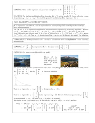
![NONLINEAR DYNAMICAL SYSTEMS Math 21b, O. Knill
SUMMARY. For linear systems x = Ax, the eigenvalues of A determine the behavior completely. For nonlinear
˙
systems explicit formulas for solutions are no more available in general. It even also happen that orbits go go
off to infinity in finite time like in x = x2 with solution x(t) = −1/(t − x(0)). With x(0) = 1 it reaches infinity
˙
at time t = 1. Linearity is often too crude. The exponential growth x = ax of a bacteria colony for example is
˙
slowed down due to lack of food and the logistic model x = ax(1 − x/M ) would be more accurate, where M
˙
is the population size for which bacteria starve so much that the growth has stopped: x(t) = M , then x(t) = 0.
˙
Nonlinear systems can be investigated with qualitative methods. In 2 dimensions x = f (x, y), y = g(x, y),
˙ ˙
where chaos does not happen, the analysis of equilibrium points and linear approximation at those
points in general allows to understand the system. Also in higher dimensions, where ODE’s can have chaotic
solutions, the analysis of equilibrium points and linear approximation at those points is a place, where linear
algebra becomes useful.
EQUILIBRIUM POINTS. A point x0 is called an equilibrium point of x = f (x) if f (x0 ) = 0. If x(0) = x0
˙
then x(t) = x0 for all times. The system x = x(6−2x−y), y = y(4−x−y) for example has the four equilibrium
˙ ˙
points (0, 0), (3, 0), (0, 4), (2, 2).
∂
JACOBIAN MATRIX. If x0 is an equilibrium point for x = f (x) then [A]ij =
˙ ∂xj fi (x) is called the Jacobian
at x0 . For two dimensional systems
∂f ∂f
x
˙ = f (x, y) ∂x (x, y) ∂y (x, y)
this is the 2 × 2 matrix A= ∂g ∂g .
˙
y = g(x, y) ∂x (x, y) ∂y (x, y)
The linear ODE y = Ay with y = x − x0 approximates the nonlinear system well near the equilibrium point.
˙
The Jacobian is the linear approximation of F = (f, g) near x 0 .
VECTOR FIELD. In two dimensions, we can draw the vector field by hand: attaching a vector (f (x, y), g(x, y))
at each point (x, y). To find the equilibrium points, it helps to draw the nullclines {f (x, y) = 0}, {g(x, y) = 0}.
The equilibrium points are located on intersections of nullclines. The eigenvalues of the Jacobeans at equilibrium
points allow to draw the vector field near equilibrium points. This information is sometimes enough to draw
the vector field by hand.
MURRAY SYSTEM (see handout) x = x(6 − 2x − y), y = y(4 − x − y) has the nullclines x = 0, y = 0, 2x + y =
˙ ˙
6, x + y = 5. There are 4 equilibrium points (0, 0), (3, 0), (0, 4), (2, 2). The Jacobian matrix of the system at
6 − 4x0 − y0 −x0
the point (x0 , y0 ) is . Note that without interaction, the two systems would be
−y0 4 − x0 − 2y0
logistic systems x = x(6 − 2x), y = y(4 − y). The additional −xy is the competition.
˙ ˙
Equilibrium Jacobean Eigenvalues Nature of equilibrium
6 0
(0,0) λ1 = 6, λ2 = 4 Unstable source
0 4
−6 −3
(3,0) λ1 = −6, λ2 = 1 Hyperbolic saddle
0 1
2 0
(0,4) λ1 = 2, λ2 = −4 Hyperbolic saddle
−4 −4
−4 −2 √
(2,2) λi = −3 ± 5 Stable sink
−2 −2
USING TECHNOLOGY (Example: Mathematica). Plot the vector field:
Needs["Graphics‘PlotField‘"]
f[x_,y_]:={x(6-2x-y),y(5-x-y)};PlotVectorField[f[x,y],{x,0,4},{y,0,4}]
Find the equilibrium solutions:
Solve[{x(6-2x-y)==0,y(5-x-y)==0},{x,y}]
Find the Jacobian and its eigenvalues at (2, 2):
A[{x_,y_}]:={{6-4x,-x},{-y,5-x-2y}};Eigenvalues[A[{2,2}]]
Plotting an orbit:
S[u_,v_]:=NDSolve[{x’[t]==x[t](6-2x[t]-y[t]),y’[t]==y[t](5-x[t]-y[t]),x[0]==u,y[0]==v},{x,y},{t,0,1}]
ParametricPlot[Evaluate[{x[t],y[t]}/.S[0.3,0.5]],{t,0,1},AspectRatio->1,AxesLabel->{"x[t]","y[t]"}]](https://image.slidesharecdn.com/6493617/85/Harvard_University_-_Linear_Al-59-320.jpg)
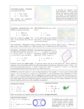
![FUNCTION SPACES/LINEAR MAPS, Math 21b, O. Knill
FROM VECTORS TO FUNCTIONS. Vectors can be displayed in different ways:
1
2 6
6
3
5
5
5 4
2
4
3
1
3
3
4
2
1
2
2 1 2 3 4 5 6
5
6
1
1 2 3 4 5 6
6
Listing the (i, vi ) can also be interpreted as the graph of a function f : 1, 2, 3, 4, 5, 6 → R, where f (i) = v i .
LINEAR SPACES. A space X in which we can add, scalar multiplications and where basic laws
like commutativity, distributivity and associativity hold is called a linear space. Examples:
• Lines, planes and more generally, the n-dimensional Euclidean space.
• Pn , the space of all polynomials of degree n.
• The space P of all polynomials.
• C ∞ , the space of all smooth functions on the line
• C 0 , the space of all continuous functions on the line.
• C 1 , the space of all differentiable functions on the line.
• C ∞ (R3 ) the space of all smooth functions in space.
• L2 the space of all functions on the line for which f 2 is integrable and
∞ 2
∞
f (x) dx < ∞.
In all these function spaces, the function f (x) = 0 which is constantly 0 is the zero function.
WHICH OF THE FOLLOWING ARE LINEAR SPACES?
The space X of all polynomials of the form f (x) = ax3 + bx4 + cx5
The space X of all continuous functions on the unit interval [−1, 1] which vanish at −1
and 1. It contains for example f (x) = x2 − |x|.
The space X of all smooth periodic functions f (x+1) = f (x). Example f (x) = sin(2πx)+
cos(6πx).
The space X = sin(x) + C ∞ (R) of all smooth functions f (x) = sin(x) + g, where g is a
smooth function.
The space X of all trigonometric polynomials f (x) = a 0 + a1 sin(x) + a2 sin(2x) + ... +
an sin(nx).
The space X of all smooth functions on R which satisfy f (1) = 1. It contains for example
f (x) = 1 + sin(x) + x.
The space X of all continuous functions on R which satisfy f (2) = 0 and f (10) = 0.
The space X of all smooth functions on R which satisfy lim |x|→∞ f (x) = 0.
The space X of all continuous functions on R which satisfy lim |x|→∞ f (x) = 1.
The space X of all smooth functions on R of compact support: for every f , there exists
an interval I such that f (x) = 0 outside that interval.
The space X of all smooth functions on R2 .](https://image.slidesharecdn.com/6493617/85/Harvard_University_-_Linear_Al-61-320.jpg)
![LINEAR TRANSFORMATIONS. A map T between linear spaces is called lin-
ear if T (x + y) = T (x) + T (y), T (λx) = λT (x), T (0) = 0. Examples:
• Df (x)= f (x) on C ∞
• T f (x) = sin(x)f (x) on C ∞
x 0
• T f (x) = 0
f (x) dx on C 1
• T f (x) = ( 0
f (x)g(x) dx)g(x) on C 0 [0, 1].
∞
• T f (x) = (f (0), f (1), f (2), f (3)) on C .
WHICH OF THE FOLLOWING MAPS ARE LINEAR TRANSFORMATIONS?
The map T (f ) = f (x) on X = C ∞ (T).
The map T (f ) = 1 + f (x) on X = C ∞ (R).
The map T (f )(x) = sin(x)f (x) on X = C ∞ (R).
The map T (f )(x) = f (x)/x on X = C ∞ (R).
x
The map T (f )(x) = 0
f (x) dx on X = C([0, 1]).
√
The map T (f )(x) = f (x + 2) on X = C ∞ (R).
∞
The map T (f )(x) = ∞
f (x − s) sin(s) ds on C 0 .
The map T (f )(x) = f (x) + f (2) on C ∞ (R).
The map T (f )(x) = f (x) + f (2) + 1 on C ∞ (R).
The map T (f )(x, y, z) = fxx (x, y, z) + fyy (x, y, z) + fzz (x, y, z) + 1/(|x|)f (x, y, z)
The map T (f )(x) = f (x2 ).
The map T (f )(x) = f (x) − x2 f (x).
The map T (f )(x) = f 2 (x) on C ∞ (R).
EIGENVALUES, BASIS, KERNEL, IMAGE. Many concepts work also here.
X linear space f, g ∈ X, f + g ∈ X, λf ∈ X, 0 ∈ X.
T linear transformation T (f + g) = T (f ) + T (g), T (λf ) = λT (f ), T (0) = 0.
f1 , f2 , ..., fn linear independent i ci fi = 0 implies fi = 0.
f1 , f2 , ..., fn span X Every f is of the form i ci fi .
f1 , f2 , ..., fn basis of X linear independent and span.
T has eigenvalue λ T f = λf
kernel of T {T f = 0}
image of T {T f |f ∈ X}.
Some concepts do not work without modification. Example: det(T ) or tr(T ) are not always defined for linear
transformations in infinite dimensions. The concept of a basis in infinite dimensions has to be defined properly.
INNER PRODUCT. The analogue of the dot product i fi gi for vectors (f1 , f2 , ..., fn ), (g1 , g2 , ..., gn ) is the
1
integral 0 f (x)g(x) dx for functions on the interval [0, 1]. One writes (f, g) and ||f || = (f, f ). This inner
1
product is defined on L2 or C ∞ ([0, 1]). Example: (x3 , x2 ) = 0 x5 dx = 1/5.
Having an inner product allows to define ”length”, ”angle” in infinite dimensions. One can use it to define
projections, Gram-Schmidt orthogonalization etc.](https://image.slidesharecdn.com/6493617/85/Harvard_University_-_Linear_Al-62-320.jpg)
![DIFFERENTIAL EQUATIONS, Math 21b, O. Knill
LINEAR DIFFERENTIAL EQUATIONS WITH CONSTANT COEFFICIENTS. Df = T f = f is a
linear map on the space of smooth functions C ∞ . If p(x) = a0 + a1 x + ... + an xn is a polynomial, then
p(D) = a0 + a1 D + ... + an Dn is a linear map on C ∞ (R) too. We will see here how to find the general solution
of p(D)f = g.
EXAMPLE. For p(x) = x2 − x + 6 and g(x) = cos(x) the problem p(D)f = g is the differential equation
f (x) − f (x) − 6f (x) = cos(x). It has the solution c1 e−2x + c2 e3x − (sin(x) + 7 cos(x))/50, where c1 , c2 are
arbitrary constants. How do we find these solutions?
THE IDEA. In general, a differential equation p(D)f = g has many solution. For example, for p(D) = D 3 , the
equation D 3 f = 0 has solutions (c0 + c1 x + c2 x2 ). The constants come from integrating three times. Integrating
means applying D −1 but since D has as a kernel the constant functions, integration gives a one dimensional
space of anti-derivatives (we can add a constant to the result and still have an anti-derivative).
In order to solve D 3 f = g, we integrate g three times. We will generalize this idea by writing T = p(D)
as a product of simpler transformations which we can invert. These simpler transformations have the form
(D − λ)f = g.
FINDING THE KERNEL OF A POLYNOMIAL IN D. How do we find a basis for the kernel of T f = f +2f +f ?
The linear map T can be written as a polynomial in D which means T = D 2 − D − 2 = (D + 1)(D − 2).
The kernel of T contains the kernel of D − 2 which is one-dimensional and spanned by f 1 = e2x . The kernel
of T = (D − 2)(D + 1) also contains the kernel of D + 1 which is spanned by f 2 = e−x . The kernel of T is
therefore two dimensional and spanned by e2x and e−x .
THEOREM: If T = p(D) = D n + an−1 Dn−1 + ... + a1 D + a0 on C ∞ then dim(ker(T )) = n.
PROOF. T = p(D) = (D − λj ), where λj are the roots of the polynomial p. The kernel of T contains the
kernel of D − λj which is spanned by fj (t) = eλj t . In the case when we have a factor (D − λj )k of T , then we
have to consider the kernel of (D − λj )k which is q(t)eλt , where q is a polynomial of degree k − 1. For example,
the kernel of (D − 1)3 consists of all functions (a + bt + ct2 )et .
T
SECOND PROOF. Write this as Ag = 0, where A is a n × n matrix and g =
˙ f, f˙, · · · , f (n−1) , where
(k) k
f = D f is the k’th derivative. The linear map T = AD acts on vectors of functions. If all eigenvalues λ j of
A are different (they are the same λj as before), then A can be diagonalized. Solving the diagonal case BD = 0
is easy. It has a n dimensional kernel of vectors F = [f 1 , . . . , fn ]T , where fi (t) = t. If B = SAS −1 , and F is in
the kernel of BD, then SF is in the kernel of AD.
REMARK. The result can be generalized to the case, when a j are functions of x. Especially, T f = g has a
solution, when T is of the above form. It is important that the function in front of the highest power D n
is bounded away from 0 for all t. For example xDf (x) = e x has no solution in C ∞ , because we can not
integrate ex /x. An example of a ODE with variable coefficients is the Sturm-Liouville eigenvalue problem
T (f )(x) = a(x)f (x) + a (x)f (x) + q(x)f (x) = λf (x) like for example the Legendre differential equation
(1 − x2 )f (x) − 2xf (x) + n(n + 1)f (x) = 0.
BACKUP
• Equations T f = 0, where T = p(D) form linear differential equations with constant coefficients
for which we want to understand the solution space. Such equations are called homogeneous. Solving
differential equations often means finding a basis of the kernel of T . In the above example, a
general solution of f + 2f + f = 0 can be written as f (t) = a1 f1 (t) + a2 f2 (t). If we fix two values like
f (0), f (0) or f (0), f (1), the solution is unique.
• If we want to solve T f = g, an inhomogeneous equation then T −1 is not unique because we have a
kernel. If g is in the image of T there is at least one solution f . The general solution is then f + ker(T ).
For example, for T = D 2 , which has C ∞ as its image, we can find a solution to D 2 f = t3 by integrating
twice: f (t) = t5 /20. The kernel of T consists of all linear functions at + b. The general solution to D 2 = t3
is at + b + t5 /20. The integration constants parameterize actually the kernel of a linear map.](https://image.slidesharecdn.com/6493617/85/Harvard_University_-_Linear_Al-63-320.jpg)
![x −λt
THE SYSTEM T f = (D − λ)f = g has the general solution ceλx + eλx 0
e g(t) dt .
−1
The solution f = (D − λ) g is the sum of a function in the kernel and a special function.
THE SOLUTION OF (D − λ)k f = g is obtained by applying (D − λ)−1 several times on g. In particular, for
g = 0, we get: the kernel of (D − λ)k as (c0 + c1 x + ... + ck−1 xk−1 )eλx .
THEOREM. The inhomogeneous p(D)f = g has an n-dimensional space of solutions in C ∞ (R).
PROOF. To solve T f = p(D)f = g, we write the equation as (D − λ 1 )k1 (D − λ2 )k2 · · · (D − λn )kn f = g. Since
we know how to invert each Tj = (D − λj )kj , we can construct the general solution by inverting one factor T j
of T one after another.
Often we can find directly a special solution f1 of p(D)f = g and get the general solution as f1 + fh , where fh
is in the n-dimensional kernel of T .
EXAMPLE 1) T f = e3x , where T = D 2 − D = D(D − 1). We first solve (D − 1)f = e3x . It has the solution
x −t 3t
f1 = cex + ex 0
e e dt = c2 ex + e3x /2. Now solve Df = f1 . It has the solution c1 + c2 ex + e3x /6 .
EXAMPLE 2) T f = sin(x) with T = (D 2 − 2D + 1) = (D − 1)2 . We see that cos(x)/2 is a special solution.
The kernel of T = (D − 1)2 is spanned by xex and ex so that the general solution is (c1 + c2 x)ex + cos(x)/2 .
EXAMPLE 3) T f = x with T = D 2 +1 = (D−i)(D+i) has the special solution f (x) = x. The kernel is spanned
by eix and e−ix or also by cos(x), sin(x). The general solution can be written as c 1 cos(x) + c2 sin(x) + x .
EXAMPLE 4) T f = x with T = D 4 + 2D 2 + 1 = (D − i)2 (D + i)2 has the special solution f (x) = x. The
kernel is spanned by eix , xeix , e−ix , x−ix or also by cos(x), sin(x), x cos(x), x sin(x). The general solution can be
written as (c0 + c1 x) cos(x) + (d0 + d1 x) sin(x) + x .
THESE EXAMPLES FORM 4 TYPICAL CASES.
CASE 1) p(D) = (D − λ1 )...(D − λn ) with real λi . The general solution of p(D)f = g is the sum of a special
solution and c1 eλ1 x + ... + cn eλn x
CASE 2) p(D) = (D − λ)k . The general solution is the sum of a special solution and a term
(c0 + c1 x + ... + ck−1 xk−1 )eλx
CASE 3) p(D) = (D − λ)(D − λ) with λ = a + ib. The general solution is a sum of a special solution and a
term c1 eax cos(bx) + c2 eax sin(bx)
CASE 4) p(D) = (D − λ)k (D − λ)k with λ = a + ib. The general solution is a sum of a special solution and
(c0 + c1 x + ... + ck−1 xk−1 )eax cos(bx) + (d0 + d1 x + ... + dk−1 xk−1 )eax sin(bx)
We know this also from the eigenvalue problem for a matrix. We either have distinct real eigenvalues, or we
have some eigenvalues with multiplicity, or we have pairs of complex conjugate eigenvalues which are distinct,
or we have pairs of complex conjugate eigenvalues with some multiplicity.
CAS SOLUTION OF ODE’s: Example: DSolve[f [x] − f [x] == Exp[3x], f[x], x]
REMARK. (informal) Operator methods are also useful for ODEs with variable coefficients. For ex-
ample, T = H − 1 = D 2 − x2 − 1, the quantum harmonic oscillator, can be written as T =
A∗ A = AA∗ + 2 with a creation operator A∗ = (D − x) and annihilation operator A =
2
(D + x). (Hint: use the commutation relation Dx − xD = 1.) The kernel f 0 = Ce−x /2 of
A = (D + x) is also the kernel of T and so an eigenvector of T and H. It is called the vacuum.
If f is an eigenvector of H with Hf = λf , then A∗ f is an eigenvector with eigenvalue λ + 2 . Proof. Because
HA∗ − A∗ H = [H, A∗ ] = 2A∗ , we have H(A∗ f ) = A∗ Hf + [H, A∗ ]f = A∗ λf + 2A∗ f = (λ + 2)(A∗ f ). We
obtain all eigenvectors fn = A∗ fn−1 of eigenvalue 1 + 2n by applying iteratively the creation operator A ∗ on
∞
the vacuum f0 . Because every function f with f 2 dx < ∞ can be written uniquely as f = n=0 an fn , we
can diagonalize H and solve Hf = g with f = n bn /(1 + 2n)fn , where g = n bn fn .](https://image.slidesharecdn.com/6493617/85/Harvard_University_-_Linear_Al-64-320.jpg)
![FOURIER SERIES, Math 21b, O. Knill
HOW DOES IT WORK? Piecewise smooth functions f (x) on [−π, π] form a linear space. The numbers
1 π
ck = 2π −π f (x)e−ikx dx are called the Fourier coefficients of f . We can recover f from these coefficients
by f (x) = k ck eikx . When we write √ = feven + fodd , where feven (x) = (f (x) + f (−x))/2 and fodd (x) =
f
∞
((f (x) − f (−x))/2, then feven (x) = a0 / 2 + k=1 ak cos(kx) and fodd (x) = k=1 bk sin(kx). The sum of the
cos-series for feven and the sin-series for fodd up gives the real Fourier series of f . Those coefficients are
√
1 π 1 π 1 π
ak = π −π f (x) cos(kx) dx, a0 = π −π f (x)/ 2 dx, bk = π −π f (x) sin(kx) dx.
While the complex expansion is more elegant, the SUMMARY.
real expansion has the advantage that one does 1 π √
not leave the real numbers. a0 = π −π
f (x)/ 2 dx
1 π
ak = π −π
f (x) cos(kx) dx
1 π 1 π
ck = 2π −π
f (x)e−ikx dx. bk = π −π
f (x) sin(kx) dx
∞ ikx a ∞ ∞
f (x) = k=−∞ ck e . f (x) = √0 +
2 k=1 ak cos(kx) + k=1 bk sin(kx)
EXAMPLE 1. Let f (x) = x on [−π, π]. This is an odd function (f (−x)+f (x) = 0) so that it has a sin series: with
k+1
1 π ∞
bk = π −π x sin(kx) dx = π (x cos(kx)/k + sin(kx)/k 2 |π ) = 2(−1)k+1 /k we get x = k=1 2 (−1)
1
−π k sin(kx).
For example, π/2 = 2(1 − 1/3 + 1/5 − 1/7...) a formula of Leibnitz.
EXAMPLE 2. Let f (x) = cos(x) + 1/7 cos(5x). This trigonometric polynomial is already the Fourier series.
The nonzero coefficients are a1 = 1, a5 = 1/7.
EXAMPLE 3. Let f (x) = |x| on [−π, π]. This is an even function f (−x) − f (x) = 0 so that it has a cos
√ 1 π 2 π 2
series: with a0 = 1/(2 2), ak = π −π |x| cos(kx) dx = π 0 x cos(kx) dx = π (+x sin(kx)/k + cos(kx)/k 2 |π ) =0
2
π ((−1)k − 1)/k 2 for k > 0.
WHERE ARE FOURIER SERIES USEFUL? Examples:
• Partial differential equations. PDE’s like u = ¨ • Chaos theory: Quite many notions in Chaos the-
c2 u become ODE’s: uk = c2 k2 uk can be solved
¨ ory can be defined or analyzed using Fourier theory.
as uk (t) = ak sin(ckt)uk (0) and lead to solutions Examples are mixing properties or ergodicity.
u(t, x) = k ak sin(ckt) sin(kx) of the PDE.
• Quantum dynamics: Transport properties of mate-
• Sound Coefficients ak form the frequency spec- rials are related to spectral questions for their Hamil-
trum of a sound f . Filters suppress frequencies, tonians. The relation is given by Fourier theory.
equalizers transform the Fourier space, compres-
sors (i.e.MP3) select frequencies relevant to the ear. • Crystallography: X ray Diffraction patterns of
a crystal, analyzed using Fourier theory reveal the
• Analysis: a sin(kx) = f (x) give explicit expres-
k k structure of the crystal.
sions for sums which would be hard to evaluate other-
wise. The Leibnitz sum π/4 = 1 − 1/3 + 1/5 − 1/7 + ... • Probability theory: The Fourier transform χX =
(Example 1 above) is an example. E[eiX ] of a random variable is called characteristic
function. Independent case: χx+y = χx χy .
• Number theory: Example: if α is irrational, then
the fact that nα (mod1) are uniformly distributed in • Image formats: like JPG compress by cutting irrel-
[0, 1] can be understood with Fourier theory. evant parts in Fourier space.
1 π
WHY DOES IT WORK? One has a dot product on functions with f · g = 2π −π f (x)g(x) dx. The functions
ek = eikx serve as basis vectors. As in Euclidean space, where v · e k = vk is the k’th coordinate of v,
1 π
the Fourier coefficient ck = ek · f = 2π −π e−ikx f (x) dx is the k-th coordinate of f . In the same way as
we wrote v = k vk ek in Euclidean space, we have f (x) = k ck ek (x). The vectors ek are orthonormal:
1 π 1 π
2π −π ek (x)em (x) dx = 2π −π e(m−k)ix dx which is zero for m = k and 1 for m = k.
√
Also the functions 1/ 2, sin(nx), cos(nx) form an orthonormal basis with respect to the dot product
1 π
(f, g) = π −π f (x)g(x) dx. The Fourier coefficients a0 , an , bn are the coordinates of f in that basis.
Fourier basis is not the only one. An other basis which has many applications are Wavelet expansions. The
principle is the same.](https://image.slidesharecdn.com/6493617/85/Harvard_University_-_Linear_Al-65-320.jpg)
![1 π
LENGTH, DISTANCE AND ANGLE. With a dot product, one has a length ||f || 2 = f · f = 2π −π |f (x)|2 dx
and can measure distances between two functions as ||f − g|| and angles between functions f, g by cos(α) =
f ·g/(||f ||||g||). Functions are called orthogonal if (f, g) = f ·g = 0. For example, an even√
function f and an odd
√
function g are orthogonal. The functions einx form an orthonormal family. The vectors 2 cos(kx), 2 sin(kx)
form an orthonormal family, cos(kx) is in the linear space of even functions and sin(kx) in the linear space of
1 π
odd functions. If we work with sin or cos Fourier series, we use the dot product f · g = π −π
f (x)g(x) dx
√
for which the functions 1/ 2, cos(kx), sin(kx) are orthonormal.
1 π
REWRITING THE DOT PRODUCT. If f (x) = k ck eikx and g(x) = k dk eikx , then 2π −π f (x)g(x) dx =
1 −ikx
2π k,m ck e dm eimx = k ck dk . The dot product is the sum of the product √ the coordinates as in
of
√ ∞
finite dimensions. If f and g are even, then f = f0 / 2 + k=1 fk cos(kx), g = g0 / 2 + k gk cos(kx) and
1 π ∞ ∞
π π f (x)g(x) dx = k=0 fk gk . If f and g are odd, and f = k fk sin(kx), g = k=1 gk sin(kx) then
∞ 1 π ∞
(f, g) = f · g = k=1 fk gk . Especially the Perseval equality π −π
|f (x)|2 = k=1
2
fk holds. It can be useful
also to find closed formulas for the sum of some series.
EXAMPLE. f (x) = x = 2(sin(x) − sin(2x)/2 + sin(3x)/3 − sin(4x)/4 + ... has coefficients f k = 2(−1)k+1 /k and
1 π
so 4(1 + 1/4 + 1/9 + ...) = π −π
x2 dx = 2π 2 /3 or 1 + 1/4 + 1/9 + 1/16 + 1/25 + ....) = π 2 /6 .
APPROXIMATIONS.
1.2
1 If f (x) = k bk cos(kx), then fn (x) =
n
k=1 bk
cos(kx) is an approximation to f . Be- 0.4
0.8 ∞
cause ||f − fk ||2 = 2
k=n+1 bk goes to zero, the 0.3
0.6
graphs of the functions fn come for large n close to 0.2
0.4 the graph of the function f . The picture to the left 0.1
0.2
shows an approximation of a piecewise continuous 2 4 6 8 10 12
even function, the right hand side the values of the -0.1
1 π
-3 -2 -1 1 2 3 coefficients ak = π −π f (x) cos(kx) dx.
-0.2
SOME HISTORY. The Greeks approximation of planetary motion through epicycles was an early use of
Fourier theory: z(t) = eit is a circle (Aristarchus system), z(t) = eit + eint is an epicycle (Ptolemaeus system),
18’th century Mathematicians like Euler, Lagrange, Bernoulli knew experimentally that Fourier series worked.
Fourier’s (picture left) claim of the convergence of the series was con-
firmed in the 19’th century by Cauchy and Dirichlet. For continuous
functions the sum does not need to converge everywhere. However, as
the 19 year old Fej´r (picture right) demonstrated in his theses in 1900,
e
n−1
the coefficients still determine the function k=−(n−1) n−|k| fk eikx →
n
f (x) for n → ∞ if f is continuous and f (−π) = f (π). Partial differ-
ential equations, i.e. the theory of heat had sparked early research
in Fourier theory.
OTHER FOURIER TRANSFORMS. On a finite interval one obtains a series, on the line an integral, on finite
sets, finite sums. The discrete Fourier transformation (DFT) is important for applications. It can be
determined efficiently by the (FFT=Fast Fourier transform) found in 1965, reducing the n 2 steps to n log(n).
Domain Name Synthesis Coefficients
T = [−π, π) Fourier series ˆ
f (x) = k fk eikx ˆ = 1 π f (x)e−ikx dx.
fk 2π −π
∞ ˆ ˆ 1 ∞ ˆ
R = (−∞, ∞)) Fourier transforms f (x) = ∞ f (k)eikx dx f (k) = 2π ∞ f (k)e−ikx dx
n ˆ ˆ 1 n
Zn = {1, .., n} DFT fm = k=1 fk eimk2π/n fk = n m=1 fm e−ikm2π/n
All these transformations can be defined in dimension d. Then k = (k 1 , ..., kd ) etc. are vectors. 2D DFT is for
example useful in image manipulation.
COMPUTER ALGEBRA. Packages like Mathematica have the discrete Fourier transform built in
F ourier[{0.3, 0.4, 0.5}] for example, gives the DFT of a three vector. You can perform a simple Fourier analysis
yourself by listening to a sound like Play[Sin[2000 ∗ x ∗ Floor[7 ∗ x]/12], {x, 0, 20}] ...](https://image.slidesharecdn.com/6493617/85/Harvard_University_-_Linear_Al-66-320.jpg)
![HEAT AND WAVE EQUATION Math 21b, O. Knill
NOTATION. We write Tx (x, t) and Tt (x, t) for the partial derivatives with respect to x or t.
THE HEAT EQUATION. The temperature distribution T (x, t) in a metal bar [0, T ] satisfies the heat equation
Tt (x, t) = µTxx (x, t). At every point, the rate of change of the temperature is proportional to the second
derivative of x . . . T (x, t) at x. The function T (t, x) is zero at both ends of the bar and f (x) = T (0, x) is a given
initial temperature distribution.
SOLVING IT. This partial differential equation (PDE) is solved by writing T (x, t) = u(x)v(t) which leads
to v(t)u(x) = v(t)u (x) or v(t)/(µv(t)) = u (x)/u(x). Because the LHS does not depend on x and the
˙ ˙
RHS not on t, this must be a constant λ. The ODE u (x) = λu(x) is an eigenvalue problem D 2 u = λu
which has only solutions when λ = −k 2 for integers k. The eigenfunctions of D 2 are uk (x) = sin(kx). The
2
second equation v(t) = k 2 µv is solved by v(t) = e− k 2 µt so that u(x, t) = sin(kx)e−k t is a solution of the
˙
heat equation. Because linear combinations of solutions are solutions too, a general solution is of the form
∞ 2
T (x, t) = k=1 ak sin(kx)e−k t . For fixed t this is a Fourier series. The coefficients ak are determined from
∞ 2 π
f (x) = T (x, 0) = k=1 ak sin(kx), where ak = π 0 f (x) sin(kx). (The factor 2 comes from the fact that f
should be thought to be extended to an odd function on [−π, π] and the integral from [−π, 0] is the same as the
from [0, π].)
FOURIER: (Solving the heat The heat equation Tt (t, x) = µTxx (t, x) with smooth
equation was the birth of Fourier T (x, 0) = f (x), T (0, 0) = T (π, 0) = 0 has the solution
∞ −k2 µt 2 π
theory) k=1 ak sin(kx)e with ak = π 0 f (x) sin(kx) dx.
Remark. If T (0, 0) = a, T (π, 0) = b instead, then the solution is T (x, t) = T 0 (x, t)+a+bx/π, where T0 (x, t) is the
solution in the box using f0 (x) = f (x) − (a + bx/π) which satisfies f (0) = f (π) = 0. (Because T (t, x) = a + bx/π
is a solution of the heat equation, we can add it to any solution and get new solutions. This allows to tune the
boundary conditions).
EXAMPLE. f (x) = x on [−π/2, π/2 π-periodically continued has the Fourier coefficients a k =
2 π/2 2 (k−1)/2
π −π/2 x sin(kx) dx = 4/(k π)(−1) for odd k and 0 else. The solution is
∞
4(−1)m −µ(2m+1)2 t
T (x, t) = e sin((2m + 1)x) .
m=0
(2m + 1)2 π
The exponential term containing the time makes the function T (x, t) converge to 0: ”The bar cools.” The higher
frequency terms are damped faster because ”Smaller disturbances are smoothed out faster.”
VISUALIZATION. We can just plot the graph of the function T (x, t) or plot the temperature distribution for
different times ti .
1.5
1 6
0.5
4
0
0
0.2
0.4 2
0.6
0.8
10](https://image.slidesharecdn.com/6493617/85/Harvard_University_-_Linear_Al-67-320.jpg)
![DERIVATION OF THE HEAT EQUATION. The temperature T measures the
100
kinetic energy distribution of atoms, and electrons in the bar. Each particle makes
75
a random walk. We can model that as follows: assume we have n adjacent
50
25
cells containing particles and in each time step, a fraction of the particles moves
2000 4000 6000 8000 10000
randomly either to the right or to the left. If Ti (t) is the energy of particles in cell i
-25 at time t, then the energy of particles at time t + 1 is ρ (Ti−1 (t) − 2Ti (t) + Ti+1 )(t)).
2
-50
This is a discrete version of the second derivative T (x, t) ∼ (T (x + dx, t) −
2T (x, t) + T (x + dx, t))/(dx2 ).
FOURIER TRANSFORM=DIAGONALISATION OF D. Fourier theory actually diagonalizes the linear
map D: write f = ˆ
ˆ inx = S −1 f and Sf = f = (. . . , c−1 , c0 , c1 , . . .). SDS −1 f = SD
ˆ ˆ inx =
n fn e n fn e
ˆ
S n nfn e inx
== (. . . , i(−1)c−1 , 0c0 , ic1 , . . .). This means that differentiation changes the Fourier coefficients
as cn → incn . From this we see that the diagonalisation of D 2 is multiplying with −n2 . Now, if u = D 2 u, then
˙
2
˙
un = −µn2 un so that un (t) = e−n t u)n(0). The partial differential equation is transformed into a sequence of
ˆ ˆ ˆ ˆ
ordinary differential equations.
· · · · · · ·
· 2i 0 0 0 0 ·
S ˆ
f ← f becomes multiplica- · 0 i 0 0 0 ·
Differentiation of the D ↓
↓M tion with the diago- M = · 0 0 0 0 0 ·
function S −1 · 0 0 0 i 0 ·
Df → M f ˆ nal matrix
· 0 0 0 0 2i ·
· · · · · · ·
WAVE EQUATION. The wave equation Ttt (x, t) = c2 Txx (x, t) is solved in a similar way as the heat equation:
writing T (x, t) = u(x)v(t) gives v u = c2 vu or v /(c2 v) = u /u. Because the left hand is independent of x
¨ ¨
and the right hand side is independent of t, we have v /(c 2 v) = u /u = −k 2 = const. The right equation
¨
has solutions uk (x) = sin(kx). Now, vk (t) = ak cos(kct) + bk sin(kct) solves v = −c2 k 2 v so that Tk (x, t) =
¨
uk (x)vk (t) = sin(kx)(ak cos(kct) + bk sin(kct)) is a solution of the wave equation. General solutions can be
∞
obtained by taking superpositions of these waves T (x, t) = k=1 ak (sin(kx) cos(kct) + bk sin(kx) sin(kct).
∞ ˙ ∞
The coefficients ak , bk are obtained from T (x, 0) = k=1 ak sin(kx) and T (x, 0) = k=1 kcbk sin(kx). Unlike in
˙
the heat equation both T (x, 0) and T (x, 0) have to be specified.
˙
The wave equation Ttt = c2 Txx with smooth T (x, 0) = f (x), T (x, 0) = g(x), T (0, 0) =
WAVE ∞
T (π, 0) = 0 has the solution k=1 ak sin(kx) cos(kct) + bk sin(kx) sin(kct) with ak =
EQUATION: 2 π 2 π
π 0 f (x) sin(kx) dx and kcbk = π 0 g(x) sin(kx) dx.
· · · · · · ·
QUANTUM MECHANICS = MA- · −4 0 0 0
0 ·
TRIX MECHANICS A particle in · 0 −1 0 0
0 · The diagonal entries are
a box is described by a linear map
2 2
h2
M = 2m · 0
¯
0 0 0 0 · the eigenvalues of L as
L = −D h /(2m) acting on func-
¯ · 0
0 0 −1 0 · usual after diagonalisa-
tions on [0, π]. In the Fourier pic- · 0 0 0 0 −4 · tion.
ture, this linear map is
· · · · · · ·
Quantum mech. observables are symmetric linear maps: for example: position, X : f → xf , momentum
P : f → i¯ f , kinetic energy f → P 2 /2m = −¯ 2 ∆/(2m), Coulomb potential energy f → (4π 0 )−1 e2 /rf .
h h
HIGHER DIMENSIONS. The heat or wave equations can be solved also in higher dimensions using Fourier
theory. For example, on a matellic plate [−π, π] × [−π, π] the temperature distribution T (x, y, t) satisfies
Tt = µ(Txx + Tyy ).
inx+my
The Fourier series of a function f (x, y) in two variables is n,m cn,m e , where cn,m =
−2 π π −inx −imy
(2π) −π −π
f (x, y)e e dx dy.
The Gaussian blur filter applied to each color coordinate of a picture acts very similar than the heat flow.](https://image.slidesharecdn.com/6493617/85/Harvard_University_-_Linear_Al-68-320.jpg)

![A GENERAL REGION. For a general region, one uses numerical methods. One pos-
sibility is by conformal transportation: to map the region into the the disc using a
complex map F , which maps the region Ω into the disc. Solve then the problem in the
disc with boundary value T (F −1 (x, y)) on the disc.
If S(x, y) is the solution there, then T (x, y) = S(F −1 (x, y)) is the solution in the region
Ω. The picture shows the example of the Joukowski map z → (z + 1/z)/2 which has
been used in fluid dynamics (N.J. Joukowski (1847-1921) was a Russian aerodynamics
researcher.)
A tourists view on related PDE topics
POISSON EQUATION. The Poisson equation ∆f = g in a square [0, π]2 can be solved via Fourier theory: If
f (x, y) = k,m an,m cos(nx) cos(my) and g(x, y) = k,m bn,m cos(nx) cos(my), then fxx + fyy = n,m −(n2 +
m2 )an,m cos(nx) cos(my) = k,m bn,m cos(nx) cos(my), then an,m = −bn,m /(n2 − m2 ). The poisson equation
is important in electrostatics, for example to determine the electromagnetic field when the charge and current
distribution is known: ∆U (x) = −(1/ 0 )ρ, then E = U is the electric field to the charge distribution ρ(x).
EIGENVALUES. The functions sin(nx) sin(ny)
are eigenfunctions for the Laplace operator fxx +
fyy = n2 f on the disc. For a general bounded
region Ω, we can look at all smooth functions
which are zero on the boundary of Ω. The possi-
ble eigenvalues of ∆f = λf are the possible ener-
gies of a particle in Ω.
COMPLEX DYNAMICS. Also in complex dy-
namics, harmonic functions appear. Finding
properties of complicated sets like the Mandel-
brot set is done by mapping the exterior to the
outside of the unit circle. If the Mandelbrot set
is charged then the contour lines of equal poten-
tial can be obtained as the corresponding contour
lines in the disc case (where the lines are circles).
SCHRODINGER EQUATION. If H is the energy operator, then i¯ f˙ = Hf is called the Schr¨dinger equa-
¨ h o
tion. If H = −¯ 2 ∆/(2m), this looks very much like the heat equation, if there were not the i. If f is an
h
eigenvalue of H, then i¯ f˙ = λf and f (t) = ei¯ t f (0). In the heat equation, we would get f (t) = e−µ(t) f (0). The
h h
evolution of the Schr¨dinger equation is very smilar to the wave equation.
o
QUANTUM CHAOS studies the eigenvalues and eigenvectors of the Laplacian in a
bounded region. If the billiard in the region is chaotic, the study of the eigensystem is
called quantum chaos. The eigenvalue problem ∆f = λf and the billiard problem
in the region are related. A famous open problem is whether two smooth convex
regions in the plane for which the eigenvalues λj are the same are equivalent up to
rotation and translation.
2
π
In a square of size L we know all the eigenvalues L2 (n2 + m2 ). The eigenvectors are
sin( pi nx) sin( pi mx). We have explicit formulas for the eigenfunctions and eigenvalues.
L L
On the classical level, for the billiard, we have also a complete picture, how a billiard
path will look like. The square is an example, where we have no quantum chaos.](https://image.slidesharecdn.com/6493617/85/Harvard_University_-_Linear_Al-70-320.jpg)