Download as PDF, PPTX


![A.A. 2012/2013Tecniche di programmazione88
Algorithm(II)
current = start state
for time = 1 to forever do
T = schedule[time]
if T = 0 return current
next = a randomly chosen successor of current
dE = value(next) – value(current)
if dE > 0 then current = next
else current = next with probability edE/T
end for](https://image.slidesharecdn.com/01-search-optimization-130528163956-phpapp02/85/Search-and-Optimization-Strategies-50-320.jpg)


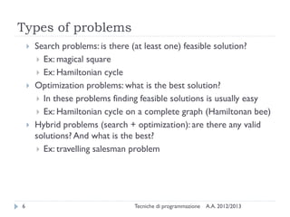
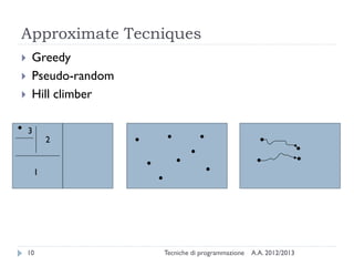
The document provides an overview of search and optimization strategies in programming, covering definitions, classifications, and techniques such as branch and bound, greedy algorithms, and local search. It details the differences between search problems, optimization problems, and hybrid problems, while also explaining various algorithmic approaches and their respective advantages and disadvantages. Additionally, it discusses advanced methods including evolutionary algorithms, genetic algorithms, and simulated annealing.