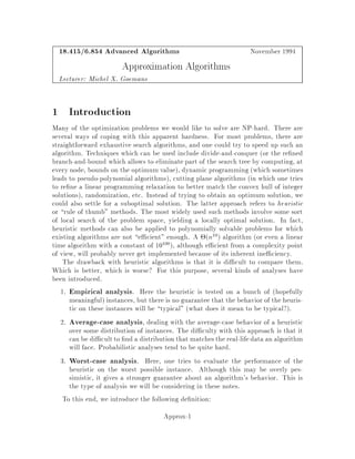
This document contains lecture notes for an advanced algorithms course taught in fall 1994 at MIT. The notes were compiled based on student scribing from previous years and cover topics like online algorithms, randomized algorithms, linear programming, network flows, and approximation algorithms. The notes are intended as an aid for teaching and learning advanced algorithm design and analysis.


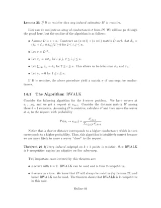


![Script md a[1]](https://cdn.slidesharecdn.com/ss_thumbnails/script-mda1-101011070309-phpapp01-thumbnail.jpg?width=640&height=640&fit=bounds)