Project management chapter 10

Project Management for Construction
Fundamental Concepts for Owners, Engineers, Architects and Builders

Chapter 10. Fundamental Scheduling
Procedures
10.1 Relevance of Construction Schedules
In addition to assigning dates to project activities, project
scheduling is intended to match the resources of equipment,
materials and labor with project work tasks over time. Good
scheduling can eliminate problems due to production bottlenecks,
facilitate the timely procurement of necessary materials, and
otherwise insure the completion of a project as soon as possible. In
contrast, poor scheduling can result in considerable waste as
laborers and equipment wait for the availability of needed
resources or the completion of preceding tasks. Delays in the
completion of an entire project due to poor scheduling can also
create havoc for owners who are eager to start using the
constructed facilities.

10.1 Relevance of Construction
Schedules
Attitudes toward the formal scheduling of projects are often
extreme. Many owners require detailed construction schedules to
be submitted by contractors as a means of monitoring the work
progress. The actual work performed is commonly compared to the
schedule to determine if construction is proceeding satisfactorily.
After the completion of construction, similar comparisons between
the planned schedule and the actual accomplishments may be
performed to allocate the liability for project delays due to changes
requested by the owner, worker strikes or other unforeseen
circumstances.

Schedules
In contrast to these instances of reliance upon formal schedules,
many field supervisors disdain and dislike formal scheduling
procedures. In particular, the critical path method of scheduling is
commonly required by owners and has been taught in universities
for over two decades, but is often regarded in the field as irrelevant
to actual operations and a time consuming distraction. The result is
"seat-of-the-pants" scheduling that can be good or that can result in
grossly inefficient schedules and poor productivity. Progressive
construction firms use formal scheduling procedures whenever the
complexity of work tasks is high and the coordination of different
workers is required.

Schedules
Formal scheduling procedures have become much more common
with the advent of personal computers on construction sites and
easy-to-use software programs. Sharing schedule information via
the Internet has also provided a greater incentive to use formal
scheduling methods. Savvy construction supervisors often carry
schedule and budget information around with wearable or handheld
computers. As a result, the continued development of easy to use
computer programs and improved methods of presenting
schedules hav overcome the practical problems associated with
formal scheduling mechanisms. But problems with the use of
scheduling techniques will continue until managers understand
their proper use and limitations.

Schedules
A basic distinction exists between resource oriented and time
oriented scheduling techniques. For resource oriented scheduling,
the focus is on using and scheduling particular resources in an
effective fashion. For example, the project manager's main concern
on a high-rise building site might be to insure that cranes are used
effectively for moving materials; without effective scheduling in this
case, delivery trucks might queue on the ground and workers wait
for deliveries on upper floors. For time oriented scheduling, the
emphasis is on determining the completion time of the project given
the necessary precedence relationships among activities. Hybrid
techniques for resource leveling or resource constrained
scheduling in the presence of precedence relationships also exist.
Most scheduling software is time-oriented, although virtually all of
the programs have the capability to introduce resource constaints.

Schedules
This chapter will introduce the fundamentals of scheduling
methods. Our discussion will generally assume that computer
based scheduling programs will be applied. Consequently, the wide
variety of manual or mechanical scheduling techniques will not be
discussed in any detail. These manual methods are not as capable
or as convenient as computer based scheduling. With the
availability of these computer based scheduling programs, it is
important for managers to understand the basic operations
performed by scheduling programs. Moreover, even if formal
methods are not applied in particular cases, the conceptual
framework of formal scheduling methods provides a valuable
reference for a manager. Accordingly, examples involving hand
calculations will be provided throughout the chapter to facilitate
understanding.

10.2 The Critical Path Method
The most widely used scheduling technique is the critical path
method (CPM) for scheduling, often referred to as critical path
scheduling. This method calculates the minimum completion time
for a project along with the possible start and finish times for the
project activities. Indeed, many texts and managers regard critical
path scheduling as the only usable and practical scheduling
procedure. Computer programs and algorithms for critical path
scheduling are widely available and can efficiently handle projects
with thousands of activities.

The critical path itself represents the set or sequence of
predecessor/successor activities which will take the longest time to
complete. The duration of the critical path is the sum of the
activities' durations along the path. Thus, the critical path can be
defined as the longest possible path through the "network" of
project activities, as described in Chapter 9. The duration of the
critical path represents the minimum time required to complete a
project. Any delays along the critical path would imply that
additional time would be required to complete the project.

There may be more than one critical path among all the project
activities, so completion of the entire project could be delayed by
delaying activities along any one of the critical paths. For example,
a project consisting of two activities performed in parallel that each
require three days would have each activity critical for a completion
in three days.

Formally, critical path scheduling assumes that a project has been
divided into activities of fixed duration and well defined predecessor
relationships. A predecessor relationship implies that one activity
must come before another in the schedule. No resource constraints
other than those implied by precedence relationships are
recognized in the simplest form of critical path scheduling.

To use critical path scheduling in practice, construction planners often
represent a resource constraint by a precedence relation. A constraint is
simply a restriction on the options available to a manager, and a
resource constraint is a constraint deriving from the limited availability of
some resource of equipment, material, space or labor. For example, one
of two activities requiring the same piece of equipment might be
arbitrarily assumed to precede the other activity. This artificial
precedence constraint insures that the two activities requiring the same
resource will not be scheduled at the same time

Also, most critical path scheduling algorithms impose restrictions
on the generality of the activity relationships or network geometries
which are used. In essence, these restrictions imply that the
construction plan can be represented by a network plan in which
activities appear as nodes in a network, as in Figure 9-6. Nodes are
numbered, and no two nodes can have the same number or
designation. Two nodes are introduced to represent the start and
completion of the project itself.

The actual computer representation of the project schedule
generally consists of a list of activities along with their associated
durations, required resources and predecessor activities. Graphical
network representations rather than a list are helpful for
visualization of the plan and to insure that mathematical
requirements are met. The actual input of the data to a computer
program may be accomplished by filling in blanks on a screen
menu, reading an existing datafile, or typing data directly to the
program with identifiers for the type of information being provided.

With an activity-on-branch network, dummy activities may be
introduced for the purposes of providing unique activity
designations and maintaining the correct sequence of activities. A
dummy activity is assumed to have no time duration and can be
graphically represented by a dashed line in a network. Several
cases in which dummy activities are useful are illustrated in Fig. 10-
1. In Fig. 10-1(a), the elimination of activity C would mean that both
activities B and D would be identified as being between nodes 1
and 3. However, if a dummy activity X is introduced, as shown in
part (b) of the figure, the unique designations for activity B (node 1
to 2) and D (node 1 to 3) will be preserved.

Furthermore, if the problem in part (a) is changed so that activity E
cannot start until both C and D are completed but that F can start
after D alone is completed, the order in the new sequence can be
indicated by the addition of a dummy activity Y, as shown in part
(c). In general, dummy activities may be necessary to meet the
requirements of specific computer scheduling algorithms, but it is
important to limit the number of such dummy link insertions to the
extent possible.

Many computer scheduling systems support only one network
representation, either activity-on-branch or acitivity-on-node. A
good project manager is familiar with either representation.

Example 10-1: Formulating a network diagram
Suppose that we wish to form an activity network for a seven-
activity network with the following precedences:

Forming an activity-on-branch network for this set of activities might
begin be drawing activities A, B and C as shown in Figure 10-2(a).
At this point, we note that two activities (A and B) lie between the
same two event nodes; for clarity, we insert a dummy activity X and
continue to place other activities as in Figure 10-2(b). Placing
activity G in the figure presents a problem, however, since we wish
both activity D and activity E to be predecessors. Inserting an
additional dummy activity Y along with activity G completes the
activity network, as shown in Figure 10-2(c). A comparable activity-
on-node representation is shown in Figure 10-3, including project
start and finish nodes. Note that dummy activities are not required
for expressing precedence relationships in activity-on-node
networks.

10.3 Calculations for Critical Path
Scheduling
With the background provided by the previous sections, we can
formulate the critical path scheduling mathematically. We shall
present an algorithm or set of instructions for critical path
scheduling assuming an activity-on-branch project network. We
also assume that all precedences are of a finish-to-start nature, so
that a succeeding activity cannot start until the completion of a
preceding activity. In a later section, we present a comparable
algorithm for activity-on-node representations with multiple
precedence types.

Scheduling
Suppose that our project network has n+1 nodes, the initial event
being 0 and the last event being n. Let the time at which node
events occur be x1, x2,...., xn, respectively. The start of the project
at x0 will be defined as time 0. Nodal event times must be
consistent with activity durations, so that an activity's successor
node event time must be larger than an activity's predecessor node
event time plus its duration. For an activity defined as starting from
event i and ending at event j, this relationship can be expressed as
the inequality constraint, xj xi + Dij where Dij is the duration of
activity (i,j). This same expression can be written for every activity
and must hold true in any feasible schedule. Mathematically, then,
the critical path scheduling problem is to minimize the time of
project completion (xn) subject to the constraints that each node
completion event cannot occur until each of the predecessor
activities have been completed:

Scheduling

Scheduling
Rather than solving the critical path scheduling problem with a
linear programming algorithm (such as the Simplex method), more
efficient techniques are available that take advantage of the
network structure of the problem. These solution methods are very
efficient with respect to the required computations, so that very
large networks can be treated even with personal computers.
These methods also give some very useful information about
possible activity schedules. The programs can compute the earliest
and latest possible starting times for each activity which are
consistent with completing the project in the shortest possible time.
This calculation is of particular interest for activities which are not
on the critical path (or paths), since these activities might be slightly
delayed or re-scheduled over time as a manager desires without
delaying the entire project.

Scheduling
An efficient solution process for critical path scheduling based upon
node labeling is shown in Table 10-1. Three algorithms appear in
the table. The event numbering algorithm numbers the nodes (or
events) of the project such that the beginning event has a lower
number than the ending event for each activity. Technically, this
algorithm accomplishes a "topological sort" of the activities. The
project start node is given number 0. As long as the project
activities fulfill the conditions for an activity-on-branch network, this
type of numbering system is always possible. Some software
packages for critical path scheduling do not have this numbering
algorithm programmed, so that the construction project planners
must insure that appropriate numbering is done.

Scheduling
The earliest event time algorithm computes the earliest possible
time, E(i), at which each event, i, in the network can occur. Earliest
event times are computed as the maximum of the earliest start
times plus activity durations for each of the activities immediately
preceding an event. The earliest start time for each activity (i,j) is
equal to the earliest possible time for the preceding event E(i):
(10.2)

Scheduling
The earliest finish time of each activity (i,j) can be calculated by:
(10.3)
Activities are identified in this algorithm by the predecessor node
(or event) i and the successor node j. The algorithm simply requires
that each event in the network should be examined in turn
beginning with the project start (node 0).

Scheduling
The latest event time algorithm computes the latest possible time,
L(j), at which each event j in the network can occur, given the
desired completion time of the project, L(n) for the last event n.
Usually, the desired completion time will be equal to the earliest
possible completion time, so that E(n) = L(n) for the final node n.
The procedure for finding the latest event time is analogous to that
for the earliest event time except that the procedure begins with the
final event and works backwards through the project activities.

Scheduling
Thus, the earliest event time algorithm is often called a forward
pass through the network, whereas the latest event time algorithm
is the the backward pass through the network. The latest finish time
consistent with completion of the project in the desired time frame
of L(n) for each activity (i,j) is equal to the latest possible time L(j)
for the succeeding event:
(10.4)
The latest start time of each activity (i,j) can be calculated by:
(10.5)

Scheduling
The earliest start and latest finish times for each event are useful
pieces of information in developing a project schedule. Events
which have equal earliest and latest times, E(i) = L(i), lie on the
critical path or paths. An activity (i,j) is a critical activity if it satisfies
all of the following conditions:

Scheduling
Hence, activities between critical events are also on a critical path
as long as the activity's earliest start time equals its latest start
time, ES(i,j) = LS(i,j). To avoid delaying the project, all the activities
on a critical path should begin as soon as possible, so each critical
activity (i,j) must be scheduled to begin at the earliest possible start
time, E(i).

10.4 Activity Float and Schedules
A number of different activity schedules can be developed from the
critical path scheduling procedure described in the previous
section. An earliest time schedule would be developed by starting
each activity as soon as possible, at ES(i,j). Similarly, a latest time
schedule would delay the start of each activity as long as possible
but still finish the project in the minimum possible time. This late
schedule can be developed by setting each activity's start time to
LS(i,j).

Activities that have different early and late start times (i.e., ES(i,j) <
LS(i,j)) can be scheduled to start anytime between ES(i,j) and
LS(i,j) as shown in Figure 10-6. The concept of float is to use part
or all of this allowable range to schedule an activity without
delaying the completion of the project. An activity that has the
earliest time for its predecessor and successor nodes differing by
more than its duration possesses a window in which it can be
scheduled. That is, if E(i) + Dij < L(j), then some float is available in
which to schedule this activity.

Float is a very valuable concept since it represents the scheduling
flexibility or "maneuvering room" available to complete particular
tasks. Activities on the critical path do not provide any flexibility for
scheduling nor leeway in case of problems. For activities with some
float, the actual starting time might be chosen to balance work
loads over time, to correspond with material deliveries, or to
improve the project's cash flow.

Of course, if one activity is allowed to float or change in the
schedule, then the amount of float available for other activities may
decrease. Three separate categories of float are defined in critical
path scheduling:
Free float is the amount of delay which can be assigned to any one
activity without delaying subsequent activities. The free float,
FF(i,j), associated with activity (i,j) is:
(10.9)
Independent float is the amount of delay which can be assigned to
any one activity without delaying subsequent activities or restricting
the scheduling of preceding activities. Independent float, IF(i,j), for
activity (i,j) is calculated as:
(10.10)

Total float is the maximum amount of delay which can be assigned
to any activity without delaying the entire project. The total float,
TF(i,j), for any activity (i,j) is calculated as:
(10.11)

Each of these "floats" indicates an amount of flexibility associated
with an activity. In all cases, total float equals or exceeds free float,
while independent float is always less than or equal to free float.
Also, any activity on a critical path has all three values of float equal
to zero. The converse of this statement is also true, so any activity
which has zero total float can be recognized as being on a critical
path.

The various categories of activity float are illustrated in Figure 10-6
in which the activity is represented by a bar which can move back
and forth in time depending upon its scheduling start. Three
possible scheduled starts are shown, corresponding to the cases of
starting each activity at the earliest event time, E(i), the latest
activity start time LS(i,j), and at the latest event time L(i). The three
categories of float can be found directly from this figure. Finally, a
fourth bar is included in the figure to illustrate the possibility that an
activity might start, be temporarily halted, and then re-start. In this
case, the temporary halt was sufficiently short that it was less than
the independent float time and thus would not interfere with other
activities. Whether or not such work splitting is possible or
economical depends upon the nature of the activity.

As shown in Table 10-3, activity D(1,3) has free and independent
floats of 10 for the project shown in Figure 10-4. Thus, the start of
this activity could be scheduled anytime between time 4 and 14
after the project began without interfering with the schedule of other
activities or with the earliest completion time of the project. As the
total float of 11 units indicates, the start of activity D could also be
delayed until time 15, but this would require that the schedule of
other activities be restricted. For example, starting activity D at time
15 would require that activity G would begin as soon as activity D
was completed. However, if this schedule was maintained, the
overall completion date of the project would not be changed.

10.5 Presenting Project Schedules
Communicating the project schedule is a vital ingredient in
successful project management. A good presentation will greatly
ease the manager's problem of understanding the multitude of
activities and their inter-relationships. Moreover, numerous
individuals and parties are involved in any project, and they have to
understand their assignments. Graphical presentations of project
schedules are particularly useful since it is much easier to
comprehend a graphical display of numerous pieces of information
than to sift through a large table of numbers. Early computer
scheduling systems were particularly poor in this regard since they
produced pages and pages of numbers without aids to the
manager for understanding them.

A short example appears in Tables 10-5 and 10-6; in practice, a
project summary table would be much longer. It is extremely
tedious to read a table of activity numbers, durations, schedule
times, and floats and thereby gain an understanding and
appreciation of a project schedule. In practice, producing diagrams
manually has been a common prescription to the lack of automated
drafting facilities. Indeed, it has been common to use computer
programs to perform critical path scheduling and then to produce
bar charts of detailed activity schedules and resource assignments
manually. With the availability of computer graphics, the cost and
effort of producing graphical presentations has been significantly
reduced and the production of presentation aids can be automated.

Network diagrams for projects have already been introduced.
These diagrams provide a powerful visualization of the
precedences and relationships among the various project activities.
They are a basic means of communicating a project plan among
the participating planners and project monitors. Project planning is
often conducted by producing network representations of greater
and greater refinement until the plan is satisfactory.

A useful variation on project network diagrams is to draw a time-
scaled network. The activity diagrams shown in the previous
section were topological networks in that only the relationship
between nodes and branches were of interest. The actual diagram
could be distorted in any way desired as long as the connections
between nodes were not changed. In time-scaled network
diagrams, activities on the network are plotted on a horizontal axis
measuring the time since project commencement. Figure 10-8
gives an example of a time-scaled activity-on-branch diagram for
the nine activity project in Figure 10-4. In this time-scaled diagram,
each node is shown at its earliest possible time. By looking over
the horizontal axis, the time at which activity can begin can be
observed. Obviously, this time scaled diagram is produced as a
display after activities are initially scheduled by the critical path
method.

Another useful graphical representation tool is a bar or Gantt chart
illustrating the scheduled time for each activity. The bar chart lists
activities and shows their scheduled start, finish and duration. An
illustrative bar chart for the nine activity project appearing in Figure
10-4 is shown in Figure 10-9. Activities are listed in the vertical axis
of this figure, while time since project commencement is shown
along the horizontal axis. During the course of monitoring a project,
useful additions to the basic bar chart include a vertical line to
indicate the current time plus small marks to indicate the current
state of work on each activity. In Figure 10-9, a hypothetical project
state after 4 periods is shown. The small "v" marks on each activity
represent the current state of each activity.

Bar charts are particularly helpful for communicating the current
state and schedule of activities on a project. As such, they have
found wide acceptance as a project representation tool in the field.
For planning purposes, bar charts are not as useful since they do
not indicate the precedence relationships among activities. Thus, a
planner must remember or record separately that a change in one
activity's schedule may require changes to successor activities.
There have been various schemes for mechanically linking activity
bars to represent precedences, but it is now easier to use computer
based tools to represent such relationships.

Other graphical representations are also useful in project
monitoring. Time and activity graphs are extremely useful in
portraying the current status of a project as well as the existence of
activity float. For example, Figure 10-10 shows two possible
schedules for the nine activity project described in Table 9-1 and
shown in the previous figures. The first schedule would occur if
each activity was scheduled at its earliest start time, ES(i,j)
consistent with completion of the project in the minimum possible
time.

With this schedule, Figure 10-10 shows the percent of project
activity completed versus time. The second schedule in Figure 10-
10 is based on latest possible start times for each activity, LS(i,j).
The horizontal time difference between the two feasible schedules
gives an indication of the extent of possible float. If the project goes
according to plan, the actual percentage completion at different
times should fall between these curves. In practice, a vertical axis
representing cash expenditures rather than percent completed is
often used in developing a project representation of this type. For
this purpose, activity cost estimates are used in preparing a time
versus completion graph. Separate "S-curves" may also be
prepared for groups of activities on the same graph, such as
separate curves for the design, procurement, foundation or
particular sub-contractor activities.

Time versus completion curves are also useful in project
monitoring. Not only the history of the project can be indicated, but
the future possibilities for earliest and latest start times. For
example, Figure 10-11 illustrates a project that is forty percent
complete after eight days for the nine activity example. In this case,
the project is well ahead of the original schedule; some activities
were completed in less than their expected durations. The possible
earliest and latest start time schedules from the current project
status are also shown on the figure.

Graphs of resource use over time are also of interest to project
planners and managers. An example of resource use is shown in
Figure 10-12 for the resource of total employment on the site of a
project. This graph is prepared by summing the resource
requirements for each activity at each time period for a particular
project schedule. With limited resources of some kind, graphs of
this type can indicate when the competition for a resource is too
large to accommodate; in cases of this kind, resource constrained
scheduling may be necessary as described in Section 10.9.

Even without fixed resource constraints, a scheduler tries to avoid
extreme fluctuations in the demand for labor or other resources
since these fluctuations typically incur high costs for training, hiring,
transportation, and management. Thus, a planner might alter a
schedule through the use of available activity floats so as to level or
smooth out the demand for resources. Resource graphs such as
Figure 10-12 provide an invaluable indication of the potential
trouble spots and the success that a scheduler has in avoiding
them.

A common difficulty with project network diagrams is that too much
information is available for easy presentation in a network. In a
project with, say, five hundred activities, drawing activities so that
they can be seen without a microscope requires a considerable
expanse of paper. A large project might require the wall space in a
room to include the entire diagram. On a computer display, a
typical restriction is that less than twenty activities can be
successfully displayed at the same time. The problem of displaying
numerous activities becomes particularly acute when accessory
information such as activity identifying numbers or phrases,
durations and resources are added to the diagram.

One practical solution to this representation problem is to define
sets of activities that can be represented together as a single
activity. That is, for display purposes, network diagrams can be
produced in which one "activity" would represent a number of real
sub-activities. For example, an activity such as "foundation design"
might be inserted in summary diagrams. In the actual project plan,
this one activity could be sub-divided into numerous tasks with their
own precedences, durations and other attributes. These sub-
groups are sometimes termed fragnets for fragments of the full
network. The result of this organization is the possibility of
producing diagrams that summarize the entire project as well as
detailed representations of particular sets of activities.

The hierarchy of diagrams can also be introduced to the production
of reports so that summary reports for groups of activities can be
produced. Thus, detailed representations of particular activities
such as plumbing might be prepared with all other activities either
omitted or summarized in larger, aggregate activity representations.
The CSI/MASTERSPEC activity definition codes described in
Chapter 9 provide a widely adopted example of a hierarchical
organization of this type. Even if summary reports and diagrams
are prepared, the actual scheduling would use detailed activity
characteristics, of course.

An example figure of a sub-network appears in Figure 10-13.
Summary displays would include only a single node A to represent
the set of activities in the sub-network. Note that precedence
relationships shown in the master network would have to be
interpreted with care since a particular precedence might be due to
an activity that would not commence at the start of activity on the
sub-network.

The use of graphical project representations is an important and
extremely useful aid to planners and managers. Of course, detailed
numerical reports may also be required to check the peculiarities of
particular activities. But graphs and diagrams provide an invaluable
means of rapidly communicating or understanding a project
schedule. With computer based storage of basic project data,
graphical output is readily obtainable and should be used whenever
possible.

Finally, the scheduling procedure described in Section 10.3 simply
counted days from the initial starting point. Practical scheduling
programs include a calendar conversion to provide calendar dates
for scheduled work as well as the number of days from the initiation
of the project. This conversion can be accomplished by
establishing a one-to-one correspondence between project dates
and calendar dates. For example, project day 2 would be May 4 if
the project began at time 0 on May 2 and no holidays intervened. In
this calendar conversion, weekends and holidays would be
excluded from consideration for scheduling, although the planner
might overrule this feature. Also, the number of work shifts or
working hours in each day could be defined, to provide consistency
with the time units used is estimating activity durations. Project
reports and graphs would typically use actual calendar days.

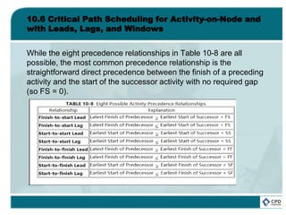
10.6 Critical Path Scheduling for Activity-on-Node and
with Leads, Lags, and Windows
Performing the critical path scheduling algorithm for activity-on-
node representations is only a small variation from the activity-on-
branch algorithm presented above. An example of the activity-on-
node diagram for a seven activity network is shown in Figure 10-3.
Some addition terminology is needed to account for the time delay
at a node associated with the task activity. Accordingly, we define:
ES(i) as the earliest start time for activity (and node) i, EF(i) is the
earliest finish time for activity (and node) i, LS(i) is the latest start
and LF(i) is the latest finish time for activity (and node) i. Table 10-7
shows the relevant calculations for the node numbering algorithm,
the forward pass and the backward pass calculations.

For manual application of the critical path algorithm shown in Table
10-7, it is helpful to draw a square of four entries, representing the
ES(i), EF(i), LS(i) and LF (i) as shown in Figure 10-14. During the
forward pass, the boxes for ES(i) and EF(i) are filled in. As an
exercise for the reader, the seven activity network in Figure 10-3
can be scheduled. Results should be identical to those obtained for
the activity-on-branch calculations.

Building on the critical path scheduling calculations described in the
previous sections, some additional capabilities are useful.
Desirable extensions include the definition of allowable windows for
activities and the introduction of more complicated precedence
relationships among activities. For example, a planner may wish to
have an activity of removing formwork from a new building
component follow the concrete pour by some pre-defined lag period
to allow setting. This delay would represent a required gap
between the completion of a preceding activity and the start of a
successor. The scheduling calculations to accommodate these
complications will be described in this section. Again, the standard
critical path scheduling assumptions of fixed activity durations and
unlimited resource availability will be made here, although these
assumptions will be relaxed in later sections.

A capability of many scheduling programs is to incorporate types of
activity interactions in addition to the straightforward predecessor
finish to successor start constraint used in Section 10.3.
Incorporation of additional categories of interactions is often called
precedence diagramming. [2] For example, it may be the case that
installing concrete forms in a foundation trench might begin a few
hours after the start of the trench excavation. This would be an
example of a start-to-start constraint with a lead: the start of the
trench-excavation activity would lead the start of the concrete-form-
placement activity by a few hours. Eight separate categories of
precedence constraints can be defined, representing greater than
(leads) or less than (lags) time constraints for each of four different
inter-activity relationships. These relationships are summarized in
Table 10-8. Typical precedence relationships would be:

• Direct or finish-to-start leads
The successor activity cannot start until the preceding activity is
complete by at least the prescribed lead time (FS). Thus, the start of a
successor activity must exceed the finish of the preceding activity by at
least FS.
• Start-to-start leads
The successor activity cannot start until work on the preceding activity
has been underway by at least the prescribed lead time (SS).
• Finish-to-finish leadss
The successor activity must have at least FF periods of work remaining
at the completion of the preceding activity.
• Start-to-finish leads
The successor activity must have at least SF periods of work remaining
at the start of the preceding activity.

While the eight precedence relationships in Table 10-8 are all
possible, the most common precedence relationship is the
straightforward direct precedence between the finish of a preceding
activity and the start of the successor activity with no required gap
(so FS = 0).

The computations with these lead and lag constraints are
somewhat more complicated variations on the basic calculations
defined in Table 10-1 for critical path scheduling. For example, a
start-to-start lead would modify the calculation of the earliest start
time to consider whether or not the necessary lead constraint was
met:
(10.12)
where SSij represents a start-to-start lead between activity (i,j) and
any of the activities starting at event j.

The possibility of interrupting or splitting activities into two work
segments can be particularly important to insure feasible schedules
in the case of numerous lead or lag constraints. With activity
splitting, an activity is divided into two sub-activities with a possible
gap or idle time between work on the two subactivities. The
computations for scheduling treat each sub-activity separately after
a split is made. Splitting is performed to reflect available scheduling
flexibility or to allow the development of a feasible schedule.

For example, splitting may permit scheduling the early finish of a
successor activity at a date later than the earliest start of the
successor plus its duration. In effect, the successor activity is split
into two segments with the later segment scheduled to finish after a
particular time. Most commonly, this occurs when a constraint
involving the finish time of two activities determines the required
finish time of the successor. When this situation occurs, it is
advantageous to split the successor activity into two so the first part
of the successor activity can start earlier but still finish in
accordance with the applicable finish-to-finish constraint.

Finally, the definition of activity windows can be extremely useful.
An activity window defines a permissible period in which a
particularly activity may be scheduled. To impose a window
constraint, a planner could specify an earliest possible start time for
an activity (WES) or a latest possible completion time (WLF). Latest
possible starts (WLS) and earliest possible finishes (WEF) might
also be imposed. In the extreme, a required start time might be
insured by setting the earliest and latest window start times equal
(WES = WLS).

These window constraints would be in addition to the time
constraints imposed by precedence relationships among the
various project activities. Window constraints are particularly useful
in enforcing milestone completion requirements on project
activities. For example, a milestone activity may be defined with no
duration but a latest possible completion time. Any activities
preceding this milestone activity cannot be scheduled for
completion after the milestone date. Window constraints are
actually a special case of the other precedence constraints
summarized above: windows are constraints in which the
precedecessor activity is the project start. Thus, an earliest
possible start time window (WES) is a start-to-start lead.

One related issue is the selection of an appropriate network
representation. Generally, the activity-on-branch representation will
lead to a more compact diagram and is also consistent with other
engineering network representations of structures or circuits. [3]
For example, the nine activities shown in Figure 10-4 result in an
activity-on-branch network with six nodes and nine branches. In
contrast, the comparable activity-on-node network shown in Figure
9-6 has eleven nodes (with the addition of a node for project start
and completion) and fifteen branches. The activity-on-node
diagram is more complicated and more difficult to draw, particularly
since branches must be drawn crossing one another. Despite this
larger size, an important practical reason to select activity-on-node
diagrams is that numerous types of precedence relationships are
easier to represent in these diagrams.

For example, different symbols might be used on each of the
branches in Figure 9-6 to represent direct precedences, start-to-
start precedences, start-to-finish precedences, etc. Alternatively,
the beginning and end points of the precedence links can indicate
the type of lead or lag precedence relationship. Another advantage
of activity-on-node representations is that the introduction of
dummy links as in Figure 10-1 is not required. Either representation
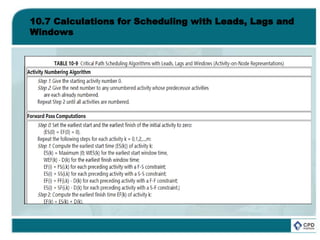
can be used for the critical path scheduling computations described
earlier. In the absence of lead and lag precedence relationships, it
is more common to select the compact activity-on-branch diagram,
although a unified model for this purpose is described in Chapter
11. Of course, one reason to pick activity-on-branch or activity-on-
node representations is that particular computer scheduling
programs available at a site are based on one representation or the
other. Since both representations are in common use, project
managers should be familiar with either network representation.

Many commercially available computer scheduling programs
include the necessary computational procedures to incorporate
windows and many of the various precedence relationships
described above. Indeed, the term "precedence diagramming" and
the calculations associated with these lags seems to have first
appeared in the user's manual for a computer scheduling program.
[4]
If the construction plan suggests that such complicated lags are
important, then these scheduling algorithms should be adopted. In
the next section, the various computations associated with critical
path scheduling with several types of leads, lags and windows are
presented.

10.7 Calculations for Scheduling with Leads, Lags and
Windows
Table 10-9 contains an algorithmic description of the calculations
required for critical path scheduling with leads, lags and windows.
This description assumes an activity-on-node project network
representation, since this representation is much easier to use with
complicated precedence relationships. The possible precedence
relationships accomadated by the procedure contained in Table 10-
9 are finish-to-start leads, start-to-start leads, finish-to-finish lags
and start-to-finish lags. Windows for earliest starts or latest finishes
are also accomodated. Incorporating other precedence and window
types in a scheduling procedure is also possible as described in
Chapter 11. With an activity-on-node representation, we assume
that an initiation and a termination activity are included to mark the
beginning and end of the project. The set of procedures described
in Table 10-9 does not provide for automatic splitting of activities.

Windows

Windows
The first step in the scheduling algorithm is to sort activities such
that no higher numbered activity precedes a lower numbered
activity. With numbered activities, durations can be denoted D(k),
where k is the number of an activity. Other activity information can
also be referenced by the activity number. Note that node events
used in activity-on-branch representations are not required in this
case.

Windows
The forward pass calculations compute an earliest start time
(ES(k)) and an earliest finish time (EF(k)) for each activity in turn
(Table 10-9). In computing the earliest start time of an activity k, the
earliest start window time (WES), the earliest finish window time
(WEF), and each of the various precedence relationships must be
considered. Constraints on finish times are included by identifying
minimum finish times and then subtracting the activity duration. A
default earliest start time of day 0 is also insured for all activities. A
second step in the procedure is to identify each activity's earliest
finish time (EF(k)).

Windows
The backward pass calculations proceed in a manner very similar
to those of the forward pass (Table 10-9). In the backward pass,
the latest finish and the latest start times for each activity are
calculated. In computing the latest finish time, the latest start time is
identified which is consistent with precedence constraints on an
activity's starting time. This computation requires a minimization
over applicable window times and all successor activities. A check
for a feasible activity schedule can also be imposed at this point: if
the late start time is less than the early start time (LS(k) < ES(k)),
then the activity schedule is not possible.

Windows
The result of the forward and backward pass calculations are the
earliest start time, the latest start time, the earliest finish time, and
the latest finish time for each activity. The activity float is computed
as the latest start time less the earliest start time. Note that window
constraints may be instrumental in setting the amount of float, so
that activities without any float may either lie on the critical path or
be constrained by an allowable window.

Windows
To consider the possibility of activity splitting, the various formulas
for the forward and backward passes in Table 10-9 must be
modified. For example, in considering the possibility of activity
splitting due to start-to-start lead (SS), it is important to ensure that
the preceding activity has been underway for at least the required
lead period. If the preceding activity was split and the first sub-
activity was not underway for a sufficiently long period, then the
following activity cannot start until the first plus the second sub-
activities have been underway for a period equal to SS(i,k). Thus,
in setting the earliest start time for an activity, the calculation takes
into account the duration of the first subactivity (DA(i)) for preceding
activities involving a start-to-start lead.

Windows
Algebraically, the term in the earliest start time calculation
pertaining to start-to-start precedence constraints (ES(i) + SS(i,k))
has two parts with the possibility of activity splitting:
where DA(i) is the duration of the first sub-activity of the preceding
activity.

Windows
The computation of earliest finish time involves similar
considerations, except that the finish-to-finish and start-to-finish lag
constraints are involved. In this case, a maximization over the
following terms is required:
Finally, the necessity to split an activity is also considered. If the
earliest possible finish time is greater than the earliest start time
plus the activity duration, then the activity must be split.

Windows
Another possible extension of the scheduling computations in
Table 10-9 would be to include a duration modification capability
during the forward and backward passes. This capability would
permit alternative work calendars for different activities or for
modifications to reflect effects of time of the year on activity
durations. For example, the duration of outside work during winter
months would be increased. As another example, activities with
weekend work permitted might have their weekday durations
shortened to reflect weekend work accomplishments.

10.8 Resource Oriented Scheduling
Resource constrained scheduling should be applied whenever
there are limited resources available for a project and the
competition for these resources among the project activities is
keen. In effect, delays are liable to occur in such cases as activities
must wait until common resources become available. To the extent
that resources are limited and demand for the resource is high, this
waiting may be considerable. In turn, the congestion associated
with these waits represents increased costs, poor productivity and,
in the end, project delays. Schedules made without consideration
for such bottlenecks can be completely unrealistic.

Resource constrained scheduling is of particular importance in
managing multiple projects with fixed resources of staff or
equipment. For example, a design office has an identifiable staff
which must be assigned to particular projects and design activities.
When the workload is heavy, the designers may fall behind on
completing their assignments. Government agencies are
particularly prone to the problems of fixed staffing levels, although
some flexibility in accomplishing tasks is possible through the
mechanism of contracting work to outside firms. Construction
activities are less susceptible to this type of problem since it is
easier and less costly to hire additional personnel for the (relatively)
short duration of a construction project. Overtime or double shift
work also provide some flexibility.

Resource oriented scheduling also is appropriate in cases in which
unique resources are to be used. For example, scheduling
excavation operations when one only excavator is available is
simply a process of assigning work tasks or job segments on a day
by day basis while insuring that appropriate precedence
relationships are maintained. Even with more than one resource,
this manual assignment process may be quite adequate. However,
a planner should be careful to insure that necessary precedences
are maintained.

Resource constrained scheduling represents a considerable
challenge and source of frustration to researchers in mathematics
and operations research. While algorithms for optimal solution of
the resource constrained problem exist, they are generally too
computationally expensive to be practical for all but small networks
(of less than about 100 nodes). [5] The difficulty of the resource
constrained project scheduling problem arises from the
combinatorial explosion of different resource assignments which
can be made and the fact that the decision variables are integer
values representing all-or-nothing assignments of a particular
resource to a particular activity. In contrast, simple critical path
scheduling deals with continuous time variables. Construction
projects typically involve many activities, so optimal solution
techniques for resource allocation are not practical.

One possible simplification of the resource oriented scheduling
problem is to ignore precedence relationships. In some
applications, it may be impossible or unnecessary to consider
precedence constraints among activities. In these cases, the focus
of scheduling is usually on efficient utilization of project resources.
To insure minimum cost and delay, a project manager attempts to
minimize the amount of time that resources are unused and to
minimize the waiting time for scarce resources. This resource
oriented scheduling is often formalized as a problem of "job shop"
scheduling in which numerous tasks are to be scheduled for
completion and a variety of discrete resources need to perform
operations to complete the tasks.

Reflecting the original orientation towards manufacturing
applications, tasks are usually referred to as "jobs" and resources
to be scheduled are designated "machines." In the provision of
constructed facilities, an analogy would be an
architectural/engineering design office in which numerous design
related tasks are to be accomplished by individual professionals in
different departments. The scheduling problem is to insure efficient
use of the individual professionals (i.e. the resources) and to
complete specific tasks in a timely manner.

The simplest form of resource oriented scheduling is a reservation
system for particular resources. In this case, competing activities or
users of a resource pre-arrange use of the resource for a particular
time period. Since the resource assignment is known in advance,
other users of the resource can schedule their activities more
effectively. The result is less waiting or "queuing" for a resource. It
is also possible to inaugurate a preference system within the
reservation process so that high-priority activities can be
accomadated directly.

In the more general case of multiple resources and specialized
tasks, practical resource constrained scheduling procedures rely on
heuristic procedures to develop good but not necessarily optimal
schedules. While this is the occasion for considerable anguish
among researchers, the heuristic methods will typically give fairly
good results. An example heuristic method is provided in the next
section. Manual methods in which a human scheduler revises a
critical path schedule in light of resource constraints can also work
relatively well. Given that much of the data and the network
representation used in forming a project schedule are uncertain,
the results of applying heuristic procedures may be quite adequate
in practice.

Example 10-6: A Reservation System [6]
A recent construction project for a high-rise building complex in New York
City was severely limited in the space available for staging materials for
hauling up the building. On the four building site, thirty-eight separate
cranes and elevators were available, but the number of movements of
men, materials and equipment was expected to keep the equipment very
busy. With numerous sub-contractors desiring the use of this equipment,
the potential for delays and waiting in the limited staging area was
considerable. By implementing a crane reservation system, these
problems were nearly entirely avoided. The reservation system required
contractors to telephone one or more days in advance to reserve time on a
particular crane. Time were available on a first-come, first-served basis
(i.e. first call, first choice of available slots). Penalties were imposed for
making an unused reservation. The reservation system was also
computerized to permit rapid modification and updating of information as
well as the provision of standard reservation schedules to be distributed to
all participants.

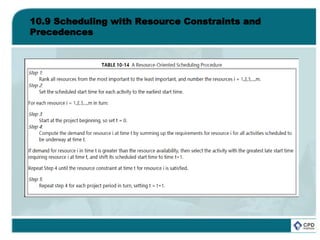
10.9 Scheduling with Resource Constraints and
Precedences
The previous section outlined resource oriented approaches to the
scheduling problem. In this section, we shall review some general
approaches to integrating both concerns in scheduling.
Two problems arise in developing a resource constrained project
schedule. First, it is not necessarily the case that a critical path
schedule is feasible. Because one or more resources might be
needed by numerous activities, it can easily be the case that the
shortest project duration identified by the critical path scheduling
calculation is impossible. The difficulty arises because critical path
scheduling assumes that no resource availability problems or
bottlenecks will arise. Finding a feasible or possible schedule is the
first problem in resource constrained scheduling. Of course, there
may be a numerous possible schedules which conform with time
and resource constraints. As a second problem, it is also desirable
to determine schedules which have low costs or, ideally, the lowest
cost.

Precedences
Numerous heuristic methods have been suggested for resource
constrained scheduling. Many begin from critical path schedules
which are modified in light of the resource constraints. Others begin
in the opposite fashion by introducing resource constraints and
then imposing precedence constraints on the activities. Still others
begin with a ranking or classification of activities into priority groups
for special attention in scheduling. [7] One type of heuristic may be
better than another for different types of problems. Certainly,
projects in which only an occasional resource constraint exists
might be best scheduled starting from a critical path schedule. At
the other extreme, projects with numerous important resource
constraints might be best scheduled by considering critical
resources first. A mixed approach would be to proceed
simultaneously considering precedence and resource constraints.

Precedences
A simple modification to critical path scheduling has been shown to be
effective for a number of scheduling problems and is simple to
implement. For this heuristic procedure, critical path scheduling is
applied initially. The result is the familiar set of possible early and late
start times for each activity. Scheduling each activity to begin at its
earliest possible start time may result in more than one activity
requiring a particular resource at the same time. Hence, the initial
schedule may not be feasible. The heuristic proceeds by identifying
cases in which activities compete for a resource and selecting one
activity to proceed. The start time of other activities are then shifted
later in time. A simple rule for choosing which activity has priority is to
select the activity with the earliest CPM late start time (calculated as
LS(i,j) = L(j)-Dij) among those activities which are both feasible (in that
all their precedence requirements are satisfied) and competing for the
resource. This decision rule is applied from the start of the project until
the end for each type of resource in turn.

Precedences
The order in which resources are considered in this scheduling
process may influence the ultimate schedule. A good heuristic to
employ in deciding the order in which resources are to be
considered is to consider more important resources first. More
important resources are those that have high costs or that are likely
to represent an important bottleneck for project completion. Once
important resources are scheduled, other resource allocations tend
to be much easier. The resulting scheduling procedure is described
in Table 10-14.

Precedences
The late start time heuristic described in Table 10-14 is only one of
many possible scheduling rules. It has the advantage of giving
priority to activities which must start sooner to finish the project on
time. However, it is myopic in that it doesn't consider trade-offs
among resource types nor the changes in the late start time that
will be occurring as activities are shifted later in time. More
complicated rules can be devised to incorporate broader
knowledge of the project schedule. These complicated rules
require greater computational effort and may or may not result in
scheduling improvements in the end.

Precedences

10.10 References
1. Au, T. Introduction to Systems Engineering--Deterministic
Models, Addison-Wesley, Reading, MA, 1973, Chapter 8.
2. Baker, K., An Introduction to Sequencing and Scheduling, John
Wiley, 1974.
3. Jackson, M.J., Computers in Construction Planning and Control,
Allen & Unwin, 1986.
4. Moder, J., C. Phillips and E. Davis, Project Management with
CPM, PERT and Precedence Diagramming, Van Nostrand
Reinhold Company, Third Edition,1983.
5. Willis, E. M., Scheduling Construction Projects, John Wiley &
Sons, 1986.

10.12 Footnotes
1. See Au, T., Introduction to Systems Engineering, Deterministic
Models, Addison-Wesley Publishing Company, Reading, MA, 1973,
for a detailed description of linear programming as a form of
mathematical optimization.
2. See K.C. Crandall, "Project Planning with Precedence Lead/Lag
Factors," Project Management Quarterly, Vol. 4, No. 3, Sept. 1973,
pp. 18-27, or J.J. Moder, C.R. Phillips, and E.W. Davis, Project
Management with CPM, PERT and Precedence Diagramming,
New York: Van Nostrand Reinhold Company, third edition, 1983,
chapter 4.

10.12 Footnotes
3. See C.T. Hendrickson and B.N. Janson, "A Common Network
Formulation of Several Civil Engineering Problems," Civil
Engineering Systems, Vol. 1, No. 4, 1984, pp. 195-203.
4. See IBM, Project Management System, Application Description
Manual, (H20-0210), IBM, 1968.
5. A variety of mathematical programming techniques have been
proposed for this problem. For a review and comparison, see J.H.
Patterson, "A Comparison of Exact Approaches for Solving the
Multiple Constrained Resource Project Scheduling Problem,"
Management Science, Vol. 30, No. 7, 1984, pp. 854-867.

10.12 Footnotes
6. This example is adapted from H. Smallowitz, "Construction by
Computer," Civil Engineering, June, 1986, pp. 71-73.
7. For discussions and comparisons of alternative heuristic
algorithms, see E.M. Davies, "An experimental investigation of
resource allocation in multiactivity projects," Operational Research
Quarterly Vol. 24, No. 11, July 1976, pp. 1186-1194; J.D. Wiest and
F.K. Levy, A Management Guide to PERT/CPM, Prentice-Hall,
New Jersey, 1977; or S.R. Lawrence, A Computational
Comparison of Heuristic Scheduling Techniques, Technical Report,
Graduate School of Industrial Administration, Carnegie-Mellon
University, 1985.

Project management chapter 10

Recommended

Recommended

More Related Content

What's hot

What's hot (19)

Similar to Project management chapter 10

Similar to Project management chapter 10 (20)

More from VancityInstitute

More from VancityInstitute (20)

Recently uploaded

Recently uploaded (20)

Project management chapter 10