Production theory

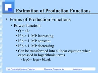
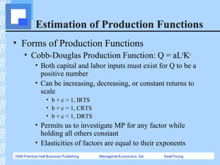
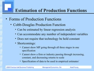
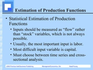
Chapter 6Chapter 6
The Theory and
Estimation of
ProductionManagerial Economics:
Economic Tools for Today’s
Decision Makers, 5/e By Paul
Keat and Philip Young

2006 Prentice Hall Business Publishing Managerial Economics, 5/e Keat/Young
The Theory and Estimation of
Production
• The Production Function
• Short-Run Analysis of Total, Average,
and Marginal Product
• Long-Run Production Function
• Estimation of Production Functions
• Importance of Production Functions in
Managerial Decision Making

Learning Objectives
• Define production function and explain
difference between short-run and long-run
production function
• Explain “law of diminishing returns” and how
it relates to the Three Stages of Production
• Define the Three Stages of Production and
explain why a rational firm always tries to
operate in Stage II

Learning Objectives
• Provide examples of types of inputs that might
go into a production function for a
manufacturing or service company
• Describe various forms of a production
function that are used in statistical estimation
of these functions
• Briefly describe the Cobb-Douglas function
and cite a few statistical studies that used this
particular functional form in their analysis

The Production Function
• Production function: defines the relationship
between inputs and the maximum amount that
can be produced within a given period of time
with a given level of technology.
• Mathematically, the production function can be
expressed as
Q=f(X1, X2, ..., Xk)
• Q: level of output
• X1, X2, ..., Xk: inputs used in the production
process

• Key assumptions
• Some given “state of the art” in the
production technology.
• Whatever input or input combinations are
included in a particular function, the output
resulting from their utilization is at the
maximum level.

• For simplicity we will often consider a
production function of two inputs:
Q=f(X, Y)
• Q: output
• X: Labor
• Y: Capital

• The short-run production function shows the
maximum quantity of good or service that can
be produced by a set of inputs, assuming the
amount of at least one of the inputs used
remains unchanged.
• The long-run production function shows the
maximum quantity of good or service that can
be produced by a set of inputs, assuming the
firm is free to vary the amount of all the inputs
being used.

Short-Run Analysis of Total,
Average, and Marginal Product
• Alternative terms in reference to inputs
• Inputs
• Factors
• Factors of production
• Resources
• Alternative terms in reference to outputs
• Output
• Quantity (Q)
• Total product (TP)
• Product

• Marginal product (MP): change in output
(or Total Product) resulting from a unit
change in a variable input.
Average Product (AP): Total Product per
unit of input used.
X
Q
MPX
∆
∆
=
X
Q
APX =

• If MP > AP then AP
is rising.
• If MP < AP then AP
is falling.
• MP=AP when AP is
maximized.

• Law of Diminishing Returns: As additional
units of a variable input are combined with a
fixed input, at some point the additional output
(i.e., marginal product) starts to diminish.
• Nothing says when diminishing returns will start to
take effect, only that it will happen at some point.
• All inputs added to the production process are
exactly the same in individual productivity

• The Three Stages of Production in the
Short Run
• Stage I: From zero units of the variable input
to where AP is maximized (where MP=AP)
• Stage II: From the maximum AP to where
MP=0
• Stage III: From where MP=0 on

• In the short run, rational firms should only be
operating in Stage II.
• Why not Stage III?
• Firm uses more variable inputs to produce less
output
• Why not Stage I?
• Underutilizing fixed capacity
• Can increase output per unit by increasing the
amount of the variable input

• What level of input usage within Stage II
is best for the firm?
• The answer depends upon how many
units of output the firm can sell, the price
of the product, and the monetary costs of
employing the variable input.

• Total Revenue Product (TRP): market value of
the firm’s output, computed by multiplying the
total product by the market price.
• TRP = Q · P
• Marginal Revenue Product (MRP): change in
the firm’s TRP resulting from a unit change in
the number of inputs used.
• MRP = = MP · PX
TRP
∆
∆

• Total Labor Cost (TLC): total cost of using the
variable input, labor, computed by multiplying
the wage rate by the number of variable inputs
employed.
• TLC = w · X
• Marginal Labor Cost (MLC): change in total
labor cost resulting from a unit change in the
number of variable inputs used. Because the
wage rate is assumed to be constant regardless
of the number of inputs used, MLC is the same
as the wage rate (w).

• Summary of relationship between demand for
output and demand for input
• A profit-maximizing firm operating in perfectly
competitive output and input markets will be using
the optimal amount of an input at the point at which
the monetary value of the input’s marginal product
is equal to the additional cost of using that input.
• MRP = MLC

• Multiple variable inputs
• Consider the relationship between the ratio
of the marginal product of one input and its
cost to the ratio of the marginal product of
the other input(s) and their cost.
• Other factors may outweigh this relationship
• Political/Economic risk factors`
k
k
w
MP
w
MP
w
MP
==
2
2
1
1

The Long-Run Production Function
• In the long run, a firm has enough time to
change the amount of all its inputs.
• Effectively, all inputs are variable.
• The long run production process is
described by the concept of returns to
scale.

• If all inputs into the production process
are doubled, three things can happen:
• output can more than double
• increasing returns to scale (IRTS)
• output can exactly double
• constant returns to scale (CRTS)
• output can less than double
• decreasing returns to scale (DRTS)

• One way to measure returns to scale is to use a
coefficient of output elasticity:
• If EQ > 1 then IRTS
• If EQ = 1 then CRTS
• If EQ < 1 then DRTS
inputsallinchangePercentage
QinchangePercentage
=QE

• Returns to scale can also be described
using the following equation
hQ = f(kX, kY)
• If h > k then IRTS
• If h = k then CRTS
• If h < k then DRTS

• Graphically, the returns to scale concept
can be illustrated using the following
graphs.
Q
X,Y
IRTS
Q
X,Y
CRTS
Q
X,Y
DRTS

Estimation of Production Functions
• Forms of Production Functions
• Short run: existence of a fixed factor to which is
added a variable factor
• One variable, one fixed factor
• Q = f(L)K
• Increasing marginal returns followed by decreasing
marginal returns
• Cubic function
• Q = a + bL + cL2
– dL3
• Diminishing marginal returns, but no Stage I
• Quadratic function
• Q = a + bL - cL2

• Power function
• Q = aLb
• If b > 1, MP increasing
• If b = 1, MP constant
• If b < 1, MP decreasing
• Can be transformed into a linear equation when
expressed in logarithmic terms
• logQ = loga + bLogL

• Cobb-Douglas Production Function: Q = aLb
Kc
• Both capital and labor inputs must exist for Q to be a
positive number
• Can be increasing, decreasing, or constant returns to
scale
• b + c > 1, IRTS
• b + c = 1, CRTS
• b + c < 1, DRTS
• Permits us to investigate MP for any factor while
holding all others constant
• Elasticities of factors are equal to their exponents

• Cobb-Douglas Production Function
• Can be estimated by linear regression analysis
• Can accommodate any number of independent variables
• Does not require that technology be held constant
• Shortcomings:
• Cannot show MP going through all three stages in one
specification
• Cannot show a firm or industry passing through increasing,
constant, and decreasing returns to scale
• Specification of data to be used in empirical estimates`

• Statistical Estimation of Production
Functions
• Inputs should be measured as “flow” rather
than “stock” variables, which is not always
possible.
• Usually, the most important input is labor.
• Most difficult input variable is capital.
• Must choose between time series and cross-
sectional analysis.

• Aggregate Production Functions
• Many studies using Cobb-Douglas did not deal
with individual firms, rather with aggregations of
industries or an economy.
• Gathering data for aggregate functions can be
difficult.
• For an economy: GDP could be used
• For an industry: data from Census of Manufactures or
production index from Federal Reserve Board
• For labor: data from Bureau of Labor Statistics

Importance of Production Functions in
Managerial Decision Making
• Production levels do not depend on how much
a company wants to produce, but on how much
its customers want to buy.
• Capacity Planning: planning the amount of
fixed inputs that will be used along with the
variable inputs. Good capacity planning
requires:
• Accurate forecasts of demand
• Effective communication between the production
and marketing functions

Production theory

More Related Content

What's hot

Similar to Production theory

Production theory