1) The document discusses factors that determine economic output, including inputs like capital and labor, and their productivity. It develops a production function model. 2) A production function relates the quantity of output to quantities of inputs like capital and labor. It has properties like being upward sloping and becoming flatter at higher input levels. 3) The document then examines labor demand and supply to determine equilibrium employment and output in an economy.

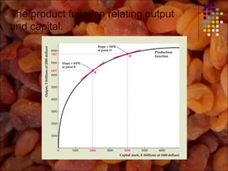
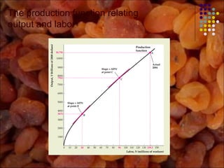
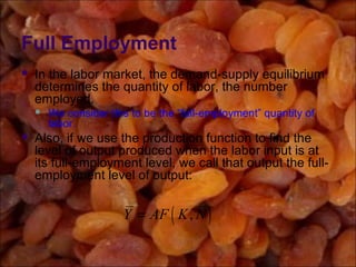
1. Productivity,
Output,
and
Employment

2. Introduction
We describes factors that determine
the level of output produced in an
economy.
It also begins to develop our theory of
the economy.

3. The Production Function
 Output produced in an economy depends on:
 The amounts of inputs available, for example
capital and labor, also raw materials
 The effectiveness with which these inputs are
used

4. The Production Function in
Equation Form

5. Production Function
Properties
 We normally plot output as a function of one
input, holding other inputs conceptually fixed.
 The production function is upward sloping (as
we plot output versus an input, e.g. capital).
 The production function becomes flatter as
we move from left to right (increasing labor
and output)

6. The product function relating output
and capital.

7. The production function relating
output and labor

8. Marginal Products

9. Supply Shocks
 Our production function shows that output is
a function of capital and labor inputs
 However, this function is subject to change
as a result of:
 Technological change
 Changes in regulatory environment
 Changes in the supply of inputs other than capital
and labor (e.g., energy)

10. Curve Shifts
 The production function is a multivariable
function
 Output depends on capital, labor, the productivity
parameter, and (implicitly) other omitted variables
 So, if we plot output versus labor, we
conceptually hold the other variables fixed
 If any of those other variables change, our plot of
the production function must shift

11. An adverse supply shock that
lowers the MPN

12. The Labor Market
 We now consider the labor market
 We will now assume that capital is fixed (in
fact, the capital stock grows slowly over time)
 In a typical business cycle, capital varies
little, but labor varies a lot

13. The Demand for Labor:
Assumptions
 The capital stock is fixed.
 Workers are all alike.
 Wages are determined in competitive labor
markets.
 Firms choose how much labor to employ in
order to maximize profit.

14. Profit Maximization and Labor
Demand
 A firm will hire an additional unit of labor so
long as the value of the extra output
produced by a worker is greater than (or just
equal to) the cost of the additional unit of
labor

15. Profit Maximization and Labor
Demand (Equations)

16. Notation

17. Profit Maximum

18. Summary

19. Demand for Labor
 At any given real wage, what quantity of labor
will a firm buy?
 Answer: The quantity that makes the marginal
product of labor equal the real wage.
 See this illustrated for one real wage rate (on the
next slide), but consider several different values
for the real wage.
 This reveals that the marginal product of labor
schedule is the firm’s labor demand schedule.

20. The determination of labor
demand

21. The Demand for Labor
 The marginal product of labor and the labor
demand curve
 Labor demand curve shows relationship between
the real wage rate and the quantity of labor
demanded
 It is the same as the MPN curve, since w = MPN
at equilibrium
 So the labor demand curve is downward sloping;
firms want to hire less labor, the higher the real
wage

22. Demand Shifters
 Factors that shift the labor demand curve
 Note: A change in the wage causes a movement
along the labor demand curve, not a shift of the
curve
 Supply shocks: Beneficial supply shock raises
MPN, so shifts labor demand curve to the right;
opposite for adverse supply shock
 Size of capital stock: Higher capital stock raises
MPN, so shifts labor demand curve to the right;
opposite for lower capital stock

23. The Economy’s Demand for
Labor
 Our preceding analysis has derived a firm’s
demand for labor function.
 Aggregate labor demand (the economy-wide
demand for labor)
 is the sum of all firms’ labor demand
 Is shifted by the same factors (supply shocks,
size of capital stock) that shift firms’ labor
demand curves

24. Labor Supply
 We now consider the supply side of the labor
market
 In microeconomics, we think of individuals as
utility maximizers
 Essentially, this means that individuals:
 have preferences that satisfy some plausible
consistency conditions
 make choices that leave them better off instead of
worse off

25. Individual Decisions about
Work
 Individuals must decide how much they wish
to work
 More work means more income (which can
be spent buying goods), but less leisure
 So when an individual decides how much to
work, she is really making a consumption
choice—she is choosing a bundle of
consisting of both “goods” and “leisure”

26. Shall I Work Another Hour?
 That depends partly on the utility I get from
the extra goods (purchased with extra labor
earnings) versus the utility lost from foregone
leisure
 It also depends partly on the real wage (the
price of leisure in terms of goods)
 Generally, if the real wage changes, this will
change an individual’s choice regarding goods
(work) and leisure.

27. Income and Substitution
Effects
 Does in increase in w (the real wage) cause an
individual to work more or less?
 An increase in w means that leisure is relatively more
expensive, leading workers to consume less leisure (work
more). This is a substitution effect.
 However, increase in w means that workers have more
purchasing power. Normally more income leads to more
consumption of both items (more goods and more leisure,
hence less work). This is an income effect.
 So the effect of an increase in w on hours worked
for an individual is theoretically ambiguous.

28. The Economy-wide Labor
Supply Curve
 Most evidence suggests that at least a short-
term or temporary increase in the real wage
(as in a business cycle fluctuation) leads to
an increase in work effort by an individual.
 Also, more individuals enter the labor force in
periods when the real wage is high.
 So, we will normally draw the labor supply
curve with an upward slope.

29. The Economy’s Labor Supply
Curve

30. Labor Supply Shifters
 Changes in wealth (or expected future wealth) will
shift the labor supply curve.
 More wealth may lead one to want both more goods and
more leisure, so work effort would fall
 If I had won the lottery last year, I might not be teaching
this class!
 Changes in population or in preferences regarding
work can also shift the labor supply curve.
Increasing in labor force participation rates of
women may partly be a response to wages, but may
also reflect changes in social norms (tastes).

31. Labor Market Equilibrium
 The equilibrium condition: The real wage
adjusts so that the quantity of labor
demanded equals the quantity of labor
supplied
( ) ( )NS w ND w=

32. Labor Market Equilibrium

33. A Favorable Supply Shock

34. Effects of A Temporary
Adverse Supply Shock

35. Full Employment
 In the labor market, the demand-supply equilibrium
determines the quantity of labor, the number
employed.
 We consider this to be the “full-employment” quantity of
labor.
 Also, if we use the production function to find the
level of output produced when the labor input is at
its full-employment level, we call that output the full-
employment level of output:
( ),Y AF K N=

36. Employment and
Unemployment
 We have referred to the employment outcome at the
demand-supply equilibrium in the labor market as a
“full-employment” outcome.
 At the same time, we know that some people are always
unemployed – so unemployment is not zero when we are
at full employment.
 Some turnover is normal even for a market in
equilibrium:
 If the number of job seekers and the number of vacancies
are evenly matched, there is no tendency for the real wage
to fall, even though positive unemployment exists.

37. Full-Employment Unemployment
(The Natural Rate)
 We know that at full employment,
unemployment is not at zero
 The unemployment rate prevailing at full-
employment is sometimes termed the
“natural rate” of unemployment