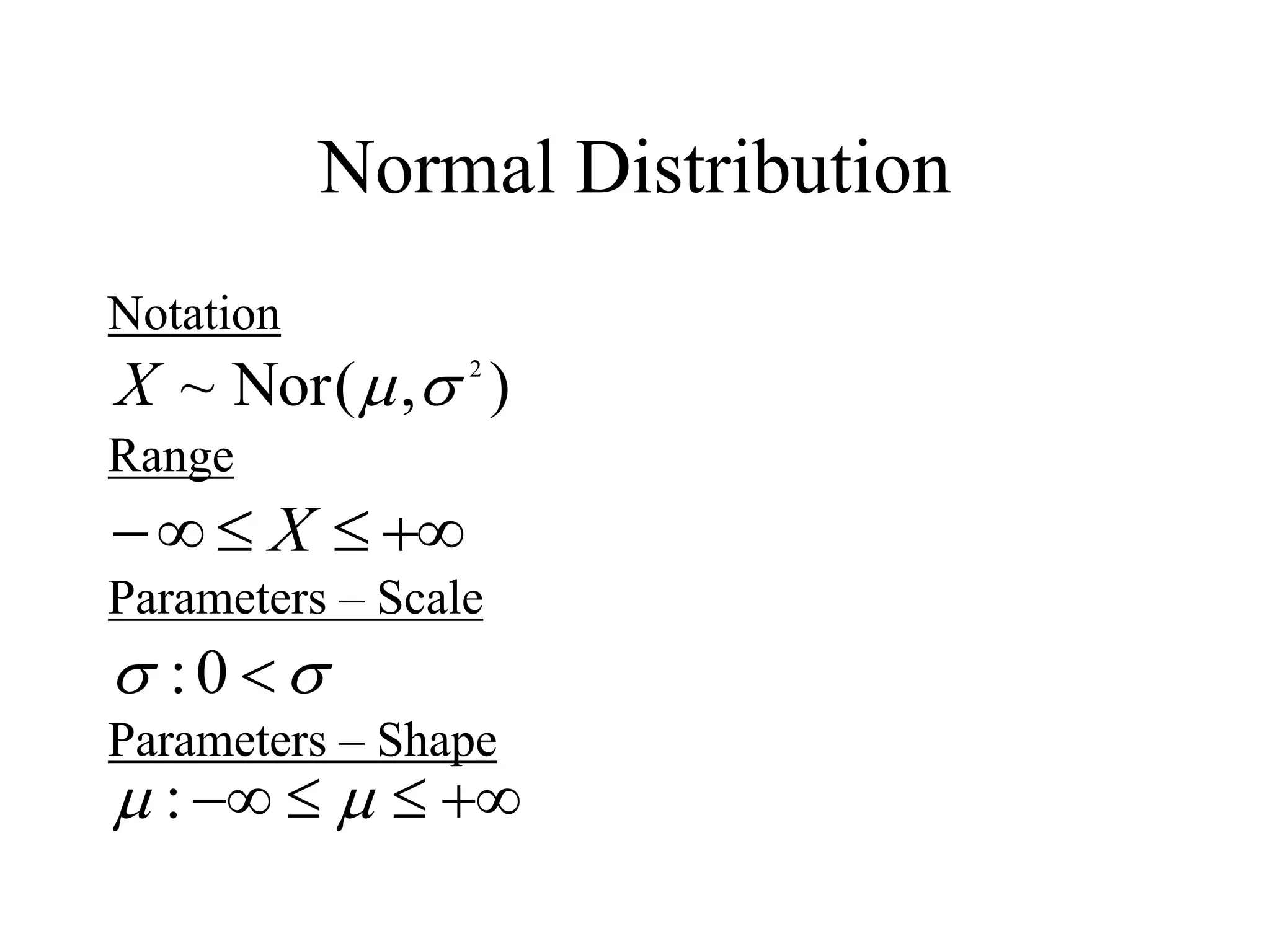
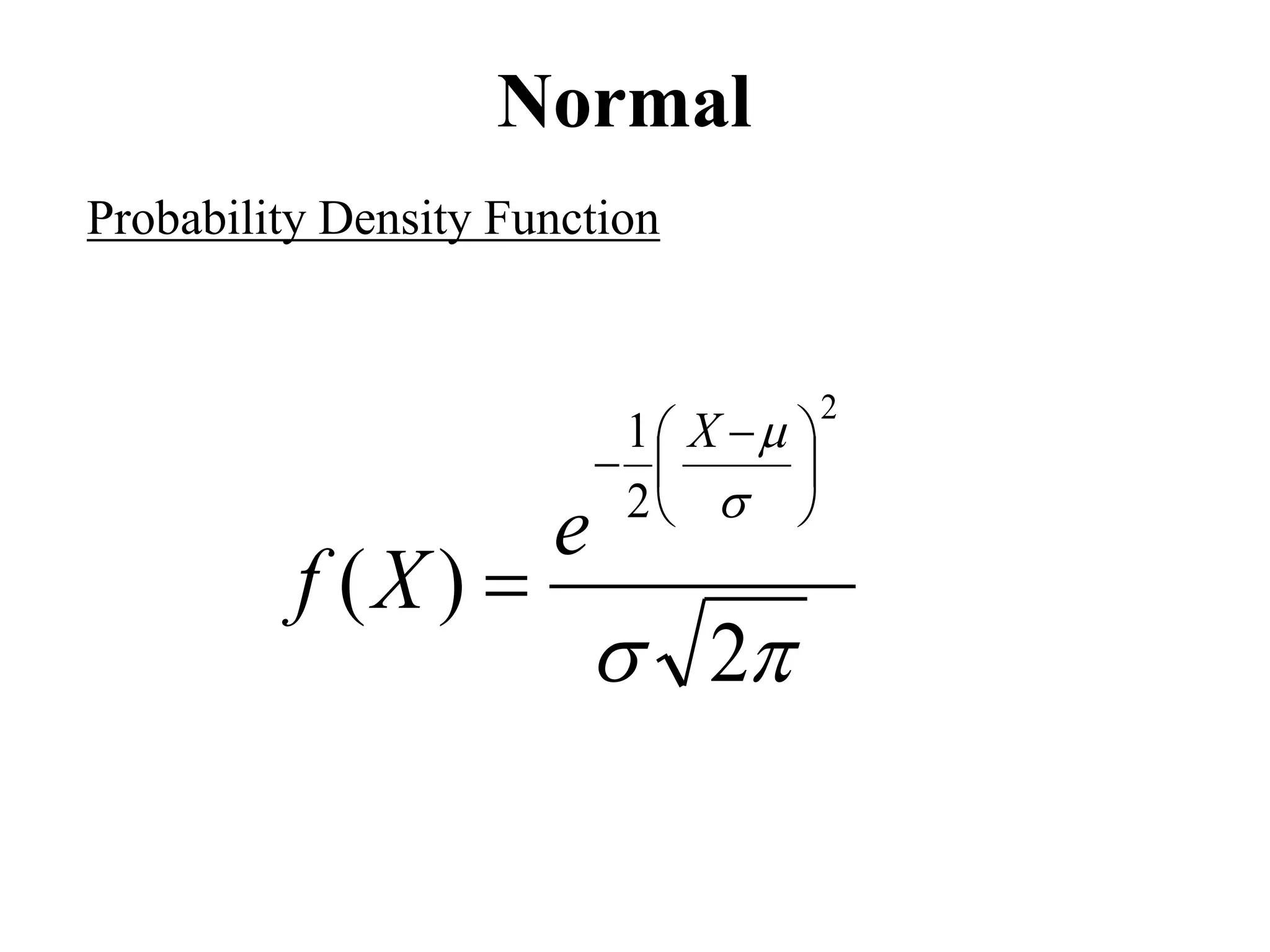
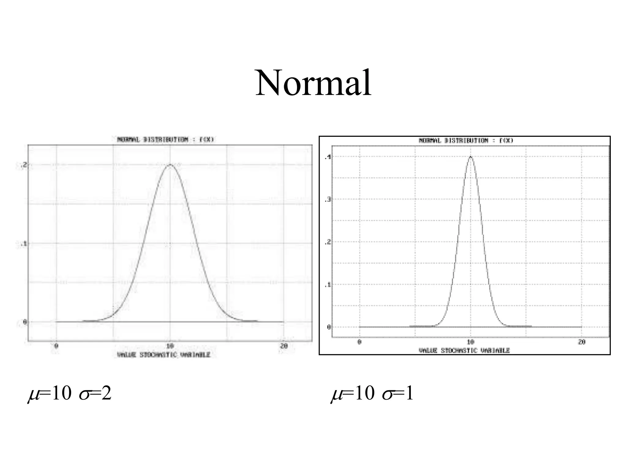
This document discusses basic probability concepts and probability distributions. It introduces probability through real-world experiments and mathematical models. Key concepts covered include sample spaces, events, probability measures, independence, random variables, probability mass functions, probability density functions, expectations, and common distributions like the normal and exponential. The normal distribution is described through its probability density function and parameters. Expectations of random variables and their properties are also summarized.

1. Probability Basic
• Introduction: Basic concepts Random experiments & events
• Elementary Theorems
• Probabilistic Modelling
• Independence
• Transformations
• Moments

2. Real-world experiments:
1. A set of possible experimental outcomes
2. A grouping of these outcomes into classes
called results
3. The relative frequency of these classes in
many independent trials of the experiment
4. Frequency is number of times the
experimental outcome falls into that class,
divided by number of times the experiment is
performed.

3. Experiment
• A random experiment: is an experiment
we do not know its exact outcome in
advance but we know the set of all possible
outcomes.

4. 1. Mathematical model: three quantities of
interest that are in one-to-one relation with the
three quantities of experimental world
2. A sample space is a collection of objects
that corresponds to the set of mutually
exclusive exhaustive outcomes of the model
of an experiment. Each object  is in the set S
is referred to as a sample point
1. A family of events  denoted {A, B,
C,…}in which each event is a set of
samples points { }

5. 3. A probability measure P which is an
assignment (mapping) of the events defined
on S into the set of real numbers. The
notation is P[A], and have these mapping
properties:
a) For any event A,0 <= P[A] <=1 (II.1)
b) P[S]=1 (II.2)
c) If A and B are “mutually exclusive” events
then P[A U B]=P[A]+P[B] (II.3)

6. • Two events A, B are said to be statistically
independent if and only if
• Theorem of total probability
If the event B is to occur it must occur in
conjunction with exactly one of the
mutually exclusive exhaustive events A
     
B
P
A
P
AB
P 
   



n
i
i B
A
P
B
P
1
i

7. • The second important form of the theorem
of total probability
     
i
n
i
i A
P
A
B
P
B
P 


1

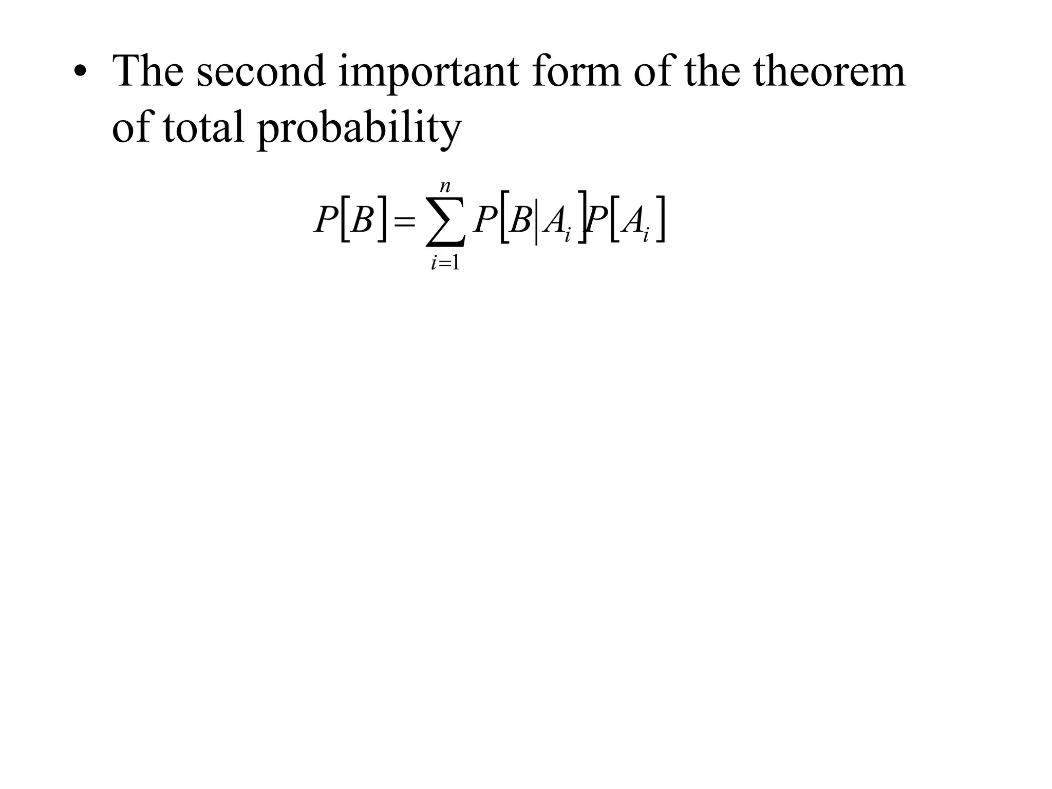
8. • Bayes’ theorem
   
 


 n
j
j
j
i
i
i
A
P
A
AB
P
A
P
A
AB
P
B
A
P
1
]
[
]
[

9. Random variables
• Random variable is a variable whose value
depends upon the outcome of a random
experiment
• To each outcome, we associate a real number,
which is in fact the value the random variable
takes on that outcome
• Random variable is a mapping from the points of
the sample space into the (real) line

10. • Example: If we win the game we win $5, if
we lose we win -$5 and if we draw we win
$0.
W
(3/8)
D
(1/4)
L
(3/8)
S
L
D
W
5
0
5
)
(















X
 
8
3
5
4
1
0
8
3
5
x
to
equal
is
)
X(
y that
probabilit
)
(
:
]
[
:
Notation












]
P[X
]
P[X
]
-
P[X
x]
P[X
x
X
x
X




11. • Probability distribution function (PDF), also
known as the cumulative distribution
function
 
b
a
for
)
(
)
(
b
a
for
b]
X
P[a
)
(
)
(
0
)
(
1
)
(
0
)
(
:
Properties
)
(
:
PDF

















a
F
b
F
a
F
b
F
F
F
x
F
x
X
P
x
F
x
x
x
x
x
x
x
X

12. +5
-5 0
x
)
(x
FX
4
1
8
3
8
3
8
5
1
0
]
4
1
[
8
5
]
6
2
[







x
P
x
P
e
upper valu
on the
takes
PDF
ity the
discontinu
of
points
At


13. • Probability density function (pdf)
• The pdf integrated over an interval gives the
probability that the random variable X lies
in that interval














1
)
(
then
1
)
(
and
0
)
(
have
We
)
(
)
(
)
(
)
(
dx
x
f
F
x
f
dy
y
f
x
F
dx
x
dF
x
f
X
X
X
x
X
X
X
X
  



b
a
X dx
x
f
b
X
a
P )
(

14. • Distributed random variable
b
a
b
a
X
b
a
X
X
x
X
x
X
e
e
dx
x
f
b
x
a
P
e
e
a
F
b
F
b
x
a
P
x
x
e
x
f
x
x
e
x
F







































 )
(
]
[
)
(
)
(
]
[
0
0
0
)
(
:
pdf
0
0
0
0
1
)
(
:
PDF

15. dx
x
f
x
dF
x
f
x
dF
x
F
)
(
)
(
)
(
)
(
pdf
and
)
(
PDF





dx
x
xf
X
X
E
x
xdF
X
X
E
X
X
)
(
]
[
)
(
]
[
is
variable
random
real
a
of
n
expectatio
The















16. • The expectation of the sum of two random
variables is always equal to the sum of the
expectations of each variable
• This is true even if the variables are dependent
• The expectation operator is a linear operator
]
[
...
]
[
]
[
]
...
[ 2
1
2
1 n
n X
E
X
E
X
E
X
X
X
E 







17. Normal Distribution
Notation
Range
Parameters – Scale
Parameters – Shape
)
,
(
Nor
~ 2


X




 X

 
0
:



 
 :

18. Normal
Probability Density Function




2
)
(
2
2
1





 


X
e
X
f

19. Normal
=10 =2 =10 =1

20. Normal
=0 =2 =0 =1

21. Normal
=0 =1

22. Normal
Expected Value


)
(X
E

23. Normal
Variance
2
)
( 

X
V

24. Exponential
Probability Density Function
Distribution Function
X
e
X
f 
 

)
(
X
e
X
F 


1
)
(