
![Heterogeneity in Structured Populations
Behavior of individuals:
time [h]
0 5 10 15 20
h(x)
-50
0
50
100
150
200
250
3 / 22](https://image.slidesharecdn.com/presentationff-170806122638/85/Presentation-OCIP-2015-3-320.jpg)
![Heterogeneity in Structured Populations
Behavior of individuals:
time [h]
0 5 10 15 20
h(x)
-50
0
50
100
150
200
250
Question
How can we mathematically describe this system?
3 / 22](https://image.slidesharecdn.com/presentationff-170806122638/85/Presentation-OCIP-2015-4-320.jpg)


![Laplace Approximation for Integral
Pinheiro [1994] suggests Laplace approximation of integral
p(Y|β, δ) ≈
ncell
k=1
ˆ
Rn
b
exp(−
1
2
Ψk (ˆbk
, β)−
1
2
(bk
−ˆbk
)T 2
bΨk (ˆbk
, β)(bk
−ˆbk
))dbk
where
Ψk (b, β, D) = −2 log p(Yk
|b, β)p(b, D)
s.t ˆbk
= arg min
b
Ψk (b, β, D) .
This approximation yields
p(Y|β, D) ≈
ncell
k=1
exp −
1
2
Ψk (ˆbk
, β) +
1
2
log (2π)nb det 2
bΨk (ˆbk
, β) .
8 / 22](https://image.slidesharecdn.com/presentationff-170806122638/85/Presentation-OCIP-2015-14-320.jpg)
![Laplace Approximation for Integral
Pinheiro [1994] suggests Laplace approximation of integral
p(Y|β, δ) ≈
ncell
k=1
ˆ
Rn
b
exp(−
1
2
Ψk (ˆbk
, β)−
1
2
(bk
−ˆbk
)T 2
bΨk (ˆbk
, β)(bk
−ˆbk
))dbk
where
Ψk (b, β, D) = −2 log p(Yk
|b, β)p(b, D)
s.t ˆbk
= arg min
b
Ψk (b, β, D) .
This approximation yields
p(Y|β, D) ≈
ncell
k=1
exp −
1
2
Ψk (ˆbk
, β) +
1
2
log (2π)nb det 2
bΨk (ˆbk
, β) .
Question
What is the corresponding inverese problem?
8 / 22](https://image.slidesharecdn.com/presentationff-170806122638/85/Presentation-OCIP-2015-15-320.jpg)

![Properties of J(ξ)
The objective function J(ξ) in general
is non-convex
is computationally expensive to evaluate
is sufficiently smooth
Proprietary implementations [Gibiansky et al., 2012] exist but
are not extendable
do not cover all desirable features
Local gradient based methods perform well in many ODE constrained
optimization problems [Raue et al., 2013]
→ Develop an efficient local gradient based optimization schemes for
mixed effect models
10 / 22](https://image.slidesharecdn.com/presentationff-170806122638/85/Presentation-OCIP-2015-17-320.jpg)
![Properties of J(ξ)
The objective function J(ξ) in general
is non-convex
is computationally expensive to evaluate
is sufficiently smooth
Proprietary implementations [Gibiansky et al., 2012] exist but
are not extendable
do not cover all desirable features
Local gradient based methods perform well in many ODE constrained
optimization problems [Raue et al., 2013]
→ Develop an efficient local gradient based optimization schemes for
mixed effect models
Question
How to compute gradients of J(ξ)?
10 / 22](https://image.slidesharecdn.com/presentationff-170806122638/85/Presentation-OCIP-2015-18-320.jpg)


![Gradient of x w.r.t. ϕ
For
∂x
∂t
= f (t, x; ϕ)
the derivatives w.r.t. ϕi can be compute via sensitivity equations:
∂
∂t
∂x
∂ϕi
= x f (t, x; ϕ)
∂x
∂ϕi
+
∂f (t, x; ϕ)
∂ϕi
∂
∂t
∂x
∂ϕi ϕj
=
∂x
∂ϕj
T
2
x f (t, x; ϕ)
∂x
∂ϕi
+ x f (t, x; ϕ)
∂x
∂ϕi ∂ϕj
+
∂f (t, x; ϕ)
∂ϕi ∂ϕj
Efficient implementation for the computation of first order sensitivities
are available in CVODES [Serban and Hindmarsh, 2005].
13 / 22](https://image.slidesharecdn.com/presentationff-170806122638/85/Presentation-OCIP-2015-21-320.jpg)

![Parametrization
∂xk
∂t
=
−ϕk
1x1
ϕk
3x − ϕk
2x
xk
(t = ϕk
4) =
1
0
ϕk
=
exp(β1)
exp(β2 + bk
1 )
exp(β3 + bk
2 )
exp(β4 + bk
3 )
bk
=
bk
1
bk
2
bk
3
∼ N
0
0
0
,
exp(δ11) 0 0
0 exp(δ22) 0
0 0 exp(δ33)
ξ = [ β1 β2 β3 β4 δ11 δ22 δ33 ]
15 / 22](https://image.slidesharecdn.com/presentationff-170806122638/85/Presentation-OCIP-2015-23-320.jpg)
![Model Description
Kallenberger et al. [2014] introduced a model for the TRAIL signalling
pathway.
This model was extended to account for new experimental data.
Number of parameters nϕ: 21
Number of states nx : 15
Number of observables ny : 6
Number of variable species nb: 8
19 / 22](https://image.slidesharecdn.com/presentationff-170806122638/85/Presentation-OCIP-2015-29-320.jpg)
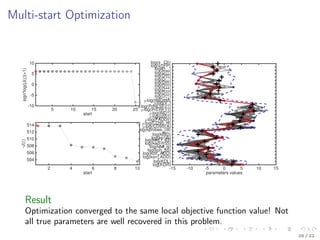


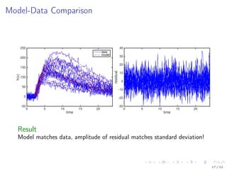
The document discusses parameter estimation for heterogeneous populations using mixed effect models, linking these models to experimental data. It presents applications to GFP transfection data and trail signaling pathways while demonstrating the development of efficient optimization methods to address challenges in estimating parameters. Additionally, it highlights the advantages of mixed effect models in computational tractability and explores various approximation and optimization techniques for parameter estimation.