This study uses high-resolution ocean model simulations to investigate subgrid dissipation and tracer dispersion in submesoscale eddy fields. It implements different subgrid mixing parameterizations to study their impact on resolved submesoscale flows and restratification. Results show enhanced dissipation occurs in localized regions at the periphery of eddies due to changes in ageostrophic shear production. Stronger eddy diffusivities reduce lateral buoyancy gradients and the rate of restratification. Salinity intrusions formed by mixed-layer eddies below the surface match observations, indicating the mechanism of tracer dispersion at submesoscales.

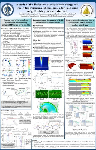
1. postersession.com
.
A study of the dissipation of eddy kinetic energy and
tracer dispersion in a submesoscale eddy field using
subgrid mixing parameterizations
Sonaljit Mukherjee1, Sanjiv Ramachandran1, Amit Tandon1, Amala Mahadevan3
University of Massachusetts Dartmouth1,Woods Hole Oceanographic Institution2
High-resolution process studies
for the Bay of Bengal
Acknowledgement
We acknowledge support from the Office of Naval Research
(N00014-09-1-0916, N00014-12-1-0101) and the National Science
Foundation (OCE-0928138). We also acknowledge computational support
from the Massachusetts Green High Performance Computing Cluster.
• Large, W. G., J. C. McWilliams, and S. C. Doney, Oceanic vertical mixing: a
review and a model with nonlocal boundary layer parameterisation, Rev.
Geophys., 32, 363–403, 1994.
• Mahadevan, A., A. Tandon, and R. Ferrari, Rapid changes in mixed layer
stratification driven by submesoscale instabilities and winds, J. Geophys.
Res., 115, C03017, doi:10.1029/2008JC005203, 2010.
Introduction
● Submesoscale processes arise near fronts and play an
important role in vertical transport of nutrients within
the mixed-layer as well as transferring energy to
smaller scales.
● Such flows are characterized by O(1) Rossby numbers
and O(1) Richardson numbers.
● 3-dimensional Ocean model simulations at fine
resolutions of O(100m to 1km) have revealed such
flows, accompanied with intense vertical velocities of
O(100m/day).
● At resolved grid scales, such flows show a dominant
balance between ageostrophic shear and dissipation of
eddy kinetic energy.
● The dynamics of turbulent fluxes in subgrid scales
needs to be explored.
.
Production and destruction of EKE
in submesoscale simulations
Introduction
● Submesoscale frontal processes play an important role in vertical
transport of nutrients within the mixed-layer and in transferring
energy to O(10m - 100m) scales.
● Such processes are characterized by O(1) Rossby numbers and
O(1) Richardson numbers.
● Three-dimensional ocean model simulations at fine resolutions
of O(100m to 1km) have resolved such processes accompanied
with intense vertical velocities of O(100m/day).
.
References
• Fox-Kemper, B., R. Ferrari., and R. Hallberg, Parameterization of Mixed Layer Eddies. Part II: Prognosis and Impact. J. Phys. Oceanogr., 38,
1166–1179, 2008.
• Mahadevan, A, Modeling vertical motion at ocean fronts: Are nonhydrostatic effects relevant at submesoscales? Ocean Modelling 14 (2006) 222–
240.
• Kunze, E., Klymak, J. M., Lien, R.-C., Ferrari, R., Lee, C. M., Sundermeyer, M. A., and Goodman, L. (2015). Submesoscale water-mass spectra in
the sargasso sea. J. Phys. Oceanogr., 45(5):1325–1338.
Objective
Previous numerical submesoscale simulations have typically
implemented ad-hoc parameterizations for vertical diffusivities.
● Study the spatial variability of subgrid dissipation in a
submesoscale eddy field.
● Contrast the impact of subgrid eddy viscosity parameterizations
on resolved submesoscale flows and restratification.
● Study the vertical structure of resolved and subgrid EKE budgets
using subgrid mixing parameterizations.
Initial condition showing the
density front (white lines),
with zonal velocity formed
due to thermal wind balance
Simulations done with PSOM
Initial mean vertical stratification
(s-2) over the frontal region
Process modeling of dispersion by
ageostrophic eddies below a
shallow mixed layer
• Flat gradient spectra of spice observed on isopycnal surfaces
below a shallow mixed layer during the Lateral Mixing
Experiment (LatMix), in June 2011 in the Sargasso Sea.
• O(1m2/s) diffusivity of tracers observed below the mixed-
layer.
• O(5km - 10km) long intrusions of salinity were observed
below the mixed-layer. What is the underlying mechanism?
Velocity and
density are in
thermal-wind
balance
Comparison of the simulated
upper-ocean properties by
different 1D mixed-layer models
Advection by mixed-layer eddies at 7th inertial period
form salinity intrusion at sub-surface depths, similar to
the ones observed during LATMIX 2011 (see below).
Observed salinity transects from LATMIX 2011 (personal
comm. with Craig Lee, APL Washington) showing
intrusions below the mixed-layer.
zonal velocity m/s
Isopycnal lines
T/S diagram obtained from LATMIX
2011. Red lines are observed profiles,
and blue lines are from the idealized
domain.
Lateral buoyancy gradient By
Salinity intrusions
Isosurface, 36.6 PSU salinity transect at 7th inertial period
Initialized fields
PSU
0C
PSU
kg/m3
Intrusions
Intrusions
z(m)
z(m)
W - E (km)
Initialized domain
density lines
Enhanced dissipation in localized
regions on the periphery of the eddies
Ageostrophic shear changes direction clockwise on the edge of the eddy
due to non-linear Ekman advection by cyclonic relative vorticity. This
deflection strengthens the total shear production on one side of the eddy
and weakens the shear production on the other side.
CONST
KEPS
KPP
ML shallows more rapidly in
KEPS
Isopycnal
slumping
Vertical
mixing
(Rudnick and Martin, 2002)
Continuous isopycnal slumping and vertical mixing reduces the lateral
buoyancy gradients, thus reducing the APE. Stronger eddy diffusivities
thus reduce the rate of restratification.
Price, Weller and Pinkel (PWP) (Price et al, 1986)
• Bulk mixed-layer model that implements convective
adjustment and a crude parameterization for shear
instability at the mixed-layer base.
K-Profile Parameterization (KPP) (Large et al, 1994)
• Calculates the surface boundary layer, and evaluates
a cubic polynomial function as an approximation for
the turbulent length scale to estimate eddy
viscosities.
k-ε (Rodi, 1976)
• Implements two time-evolving equations for subgrid
Eddy Kinetic Energy (EKE) and dissipation rate ε.
• Estimates eddy viscosities and diffusivities
separately based on the local stratification and shear.
Surface Waves Processes Program (SWAPP)
• No near-inertial shear within the mixed layer.
• Intense near-inertial shear below the mixed layer.
Marine Light-Mixed Layer Experiment (MLML)
• 22 day mixing phase followed by a 2½ month
restratification phase.
• SST elevates by 6o
C from the mixing to the
restratification phase.
SST
amplitude
Net SST
increment
• Diurnal amplitude largest for KPP, followed by k-ε and PWP.
• SST increment largest for PWP at the end of the diurnal cycle,
followed by nearly equal increments by KPP and k-ε.
• The net SST increment at the end of a diurnal cycle accumulates
over multiple diurnal cycles, forming a large SST bias between thet
PWP, and the KPP and k-ε models.
Leading order balance
between dissipation and
subgrid shear production
m
2
s
-3
×10
-6
1 1 3
CONST2
m
2
s
-3
×10
-6
-3 -1 1 3
z(m)
-30
-25
-20
-15
-10
-5
KPP
m
2
s
-3
×10
-6
-3 -1 1 3
z(m)
-30
-25
-20
-15
-10
-5
KEPS
m
2
s
-3
×10
-7
0 1 2
ONST2
m
2
s
-3
×10
-7
-2 -1 0 1 2
z(m)
-100
-80
-60
-40
-20
KPP
m
2
s
-3
×10
-7
-2 -1 0 1 2
z(m)
-100
-90
-80
-70
-60
-50
-40
-30
-20
KEPS
Ageo. shear prod.
Interscale transfer
Buoyancy prod.
Horiz. press. tran.
Vert. press. tran.
Geo. shear prod.
Advection
Sum
×10
-7
-2 3
-30
-20
-10
b) c)
e) f)
Shear-driven layer near the
surface, overlying a
buoyancy-driven layer
Subgrid EKE budget
Resolved EKE budget
Inertial and diurnal maxima
ε at 10m depth, after 10 inertial
periods
Variability of SST with depth-
integrated heat content
S-N (km)
0 50 100 150
s-2
×10
-8
-10
-5
0
∇
S-N
B
s
-2
×10
-4
0 1 2 3 4
z(m)
-400
-200
0
N
2
Cycles/km
10
-2
10
-1
10
0
10
1
Π(κ)×4π2
κ2
10
-10
10
-9
10
-8
10
-7
10
-6
10-5
10
-4
10
-3 KEPS, EKE, Along-front
25.6 kg/m
3
25.7 kg/m
3
25.8 kg/m3
25.9 kg/m3
26.0 kg/m
3
26.1 kg/m
3
Cycles/km
10
-2
10
-1
10
0
10
1
Π(κ)×4π
2
κ
2
10
-10
10
-9
10
-8
10
-7
10
-6
10-5
10
-4
10
-3 KEPS, EKE, Cross-front
25.6 kg/m
3
25.7 kg/m3
25.8 kg/m3
25.9 kg/m
3
26.0 kg/m
3
26.1 kg/m3
10
-2
10
-1
10
0
10
1
S(κ)×4π
2
κ
2
10
-10
10
-9
10
-8
10
-7
10
-6
10-5
10
-4
10
-3 KEPS, S', Along-front
25.6 kg/m
3
25.7 kg/m3
25.8 kg/m3
25.9 kg/m
3
26.0 kg/m
3
26.1 kg/m3
Cycles/km
10
-2
10
-1
10
0
10
1
S(κ)×4π
2
κ
2
10
-10
10
-9
10
-8
10
-7
10
-6
10-5
10
-4
10
-3 KEPS, S', Cross-front
25.6 kg/m3
25.7 kg/m3
25.8 kg/m
3
25.9 kg/m
3
26.0 kg/m3
26.1 kg/m3
Cycles/km
10-2
10-1
100
101
Π(κ)×4π
2
κ
2
10-10
10-9
10-8
10-7
10-6
10-5
10-4
10-3
Total and Ageo. EKE, σ
θ
=25.6 kg/m3
Along-front, Total EKE
Along-front, Ageo. EKE
Cross-front, Total EKE
Cross-front, Ageo. EKE
a) b)
d) e)
c)
Cycles/km
10
-2
10
-1
10
0
10
1
Π(κ)×4π2
κ2
10
-10
10
-9
10
-8
10
-7
10
-6
10
-5
10
-4
10
-3 KEPS, EKE, Along-front
25.6 kg/m3
25.7 kg/m3
25.8 kg/m3
25.9 kg/m3
26.0 kg/m3
26.1 kg/m
3
Cycles/km
10
-2
10
-1
10
0
10
1
Π(κ)×4π2
κ2
10
-10
10
-9
10
-8
10
-7
10
-6
10
-5
10
-4
10
-3 KEPS, EKE, Along-front
25.6 kg/m3
25.7 kg/m3
25.8 kg/m3
25.9 kg/m3
26.0 kg/m3
26.1 kg/m
3
Cycles/km
10
-2
10
-1
10
0
10
1
Π(κ)×4π
2
κ
2
10
-10
10
-9
10
-8
10
-7
10
-6
10
-5
10
-4
10
-3 KEPS, EKE, Along-front
25.6 kg/m3
25.7 kg/m3
25.8 kg/m3
25.9 kg/m3
26.0 kg/m3
26.1 kg/m
3
Cycles/km
10
-2
10
-1
10
0
10
1
Π(κ)×4π
2
κ
2
10
-10
10
-9
10
-8
10
-7
10
-6
10
-5
10
-4
10
-3 KEPS, EKE, Along-front
25.6 kg/m3
25.7 kg/m3
25.8 kg/m3
25.9 kg/m3
26.0 kg/m3
26.1 kg/m
3
Cycles/km
10-2
10-1
100
101
Π(κ)×4π
2
κ
2
10-10
10
-9
10
-8
10-7
10
-6
10-5
10
-4
10-3
Total and Ageo. EKE, σθ
=25.6 kg/m
3
Along-front, Total EKE
Along-front, Ageo. EKE
Cross-front, Total EKE
Cross-front, Ageo. EKE
Cycles/km
10-2
10-1
100
101
Π(κ)×4π
2
κ
2
10
-10
10-9
10
-8
10-7
10
-6
10-5
10
-4
10-3 KEPS, EKE, Along-front
25.6 kg/m
3
25.7 kg/m3
25.8 kg/m
3
25.9 kg/m3
26.0 kg/m
3
26.1 kg/m
3
-1
0
1/3
-1
0
1/3
-1
0
1/3
-1
0
1/3
-1
0
1/3
• Salinity spectra flatter
than the EKE spectra,
implying that salinity
is stirred by
ageostrophic eddies in
the submesoscale
range.
• Variance reduces with
depth, velocity gradient
spectral slope close to -1.
• Cross-front spectra
flatter than along-front
spectra.
• Ageostrophic EKE
spectra is flatter than the
total EKE spectra.
Salinity and velocity gradient spectra on Isopycnal surfaces below the ML
While it is expected for the mixing and dissipation to be enhanced during convective
nstability, our simulations show weaker dissipation at the destratifying edge and stronger
issipation at the restratifying edge. This is because of the parameterization of the subgrid
ixing models which result in the dissipation to be in leading order balance with the subgrid
hear production. The subgrid EKE budget from the KEPS simulation further shows that
he subgrid buoyancy production is an order of magnitude less than the shear production.
Since the parameterized ‘ in the subgrid mixing models is proportional to the shear
roduction, the destratifying edge exhibits weak dissipation despite convective instability.
5 EKE budgets at resolved and subgrid scales
n this section we study the influence of different vertical mixing parameterizations on
he spatially averaged EKE budgets at resolved and subgrid scales, where the averaging is
one over the eddying region. Since the averaged budgets in the simulations CONST2 and
ONST1 are similar, we present only the results from CONST2, KEPS and KPP.
3.5.1 Resolved EKE budget
he following equation represents the different terms of the resolved-scale EKE budget:
ˆ(uÕ
iuÕ
i)
ˆt¸ ˚˙ ˝
˙EKE
=
A
≠uj
ˆ
ˆxj
(uÕ
iuÕ
i)
B
¸ ˚˙ ˝
advection
+ ≠
Q
a(uÕ
iuÕ
j)
A
ˆui
ˆxj
B
geo
R
b ≠
Q
a(uÕ
iuÕ
j)
A
ˆui
ˆxj
B
ageo
R
b
¸ ˚˙ ˝
geo. shear production(Pgr) and ageo. shear production(Par)
+ (BÕ
uÕ
i)i=3
¸ ˚˙ ˝
buoyancy production Br
≠
1
fl0
ˆ
ˆxi
(pÕ
uÕ
i)
¸ ˚˙ ˝
pressure transport
+
A
·ij
ˆui
ˆxj
B
¸ ˚˙ ˝
interscale transfer (‘I)
, (3.16)
65
While it is expected for the mixing and dissipation to be enhanced during convective
instability, our simulations show weaker dissipation at the destratifying edge and stronger
dissipation at the restratifying edge. This is because of the parameterization of the subgrid
mixing models which result in the dissipation to be in leading order balance with the subgrid
shear production. The subgrid EKE budget from the KEPS simulation further shows that
the subgrid buoyancy production is an order of magnitude less than the shear production.
Since the parameterized ‘ in the subgrid mixing models is proportional to the shear
production, the destratifying edge exhibits weak dissipation despite convective instability.
3.5 EKE budgets at resolved and subgrid scales
In this section we study the influence of different vertical mixing parameterizations on
the spatially averaged EKE budgets at resolved and subgrid scales, where the averaging is
done over the eddying region. Since the averaged budgets in the simulations CONST2 and
CONST1 are similar, we present only the results from CONST2, KEPS and KPP.
3.5.1 Resolved EKE budget
The following equation represents the different terms of the resolved-scale EKE budget:
ˆ(uÕ
iuÕ
i)
ˆt¸ ˚˙ ˝
˙EKE
=
A
≠uj
ˆ
ˆxj
(uÕ
iuÕ
i)
B
¸ ˚˙ ˝
advection
+ ≠
Q
a(uÕ
iuÕ
j)
A
ˆui
ˆxj
B
geo
R
b ≠
Q
a(uÕ
iuÕ
j)
A
ˆui
ˆxj
B
ageo
R
b
¸ ˚˙ ˝
geo. shear production(Pgr) and ageo. shear production(Par)
+ (BÕ
uÕ
i)i=3
¸ ˚˙ ˝
buoyancy production Br
≠
1
fl0
ˆ
ˆxi
(pÕ
uÕ
i)
¸ ˚˙ ˝
pressure transport
+
A
·ij
ˆui
ˆxj
B
¸ ˚˙ ˝
interscale transfer (‘I)
, (3.16)
65
3.5.2 Subgrid EKE budget
Among the different subgrid mixing schemes considered in this study, only the k ≠ ‘
scheme allows us to explore the subgrid EKE budget since it has a transport equation for the
parameterized subgrid EKE (k). The terms governing the evolution of k are shown below:
ˆ
ˆt
k =
ˆ
ˆxi
A
‹m
‡k
ˆ
ˆxi
k
B
i=3
¸ ˚˙ ˝
downgradient transfer Dk
≠
A
ui
ˆ
ˆxi
k
B
i=1,2
¸ ˚˙ ˝
Horizontal advection Ah
+
A
≠ui
ˆ
ˆxi
k
B
i=3
¸ ˚˙ ˝
Vertical advection Av
+
A
≠·ij
ˆui
ˆxj
B
i=1,2;j=3
¸ ˚˙ ˝
shear production Ps=‹mS2
+
1
·B
i
2
i=3
¸ ˚˙ ˝
buoyancy production Bs=≠‹sN2
≠ ‘¸˚˙˝
subgrid dissipation
,
(3.17)
where ui is the resolved velocity and ·B
i is the subgrid buoyancy production. The terms Ah
and Av are the horizontal and vertical advection of k by the resolved-scale velocities. The
term Ps denotes the production of k at subgrid scales through the contraction of the subgrid
stress and the resolved-scale shear. Note that Ps is identical in magnitude but opposite in sign
to the interscale transfer term ‘I (equation 3.16), the sink in the resolved-scale EKE budget.
The term Bs is a downgradient parameterization for the subgrid buoyancy flux (Burchard
et al., 1999; Rodi, 1976). The term ‘ denotes the dissipation of EKE at the smallest scales,
which is parameterized in KEPS through a separate equation (3.5). The terms Ps and Bs
are parameterized based on the resolved shear and stratification respectively, and can be
obtained in the other subgrid mixing parameterizations as well.
70
3.5.2 Subgrid EKE budget
Among the different subgrid mixing schemes considered in this study, only the k ≠ ‘
scheme allows us to explore the subgrid EKE budget since it has a transport equation for the
parameterized subgrid EKE (k). The terms governing the evolution of k are shown below:
ˆ
ˆt
k =
ˆ
ˆxi
A
‹m
‡k
ˆ
ˆxi
k
B
i=3
¸ ˚˙ ˝
downgradient transfer Dk
≠
A
ui
ˆ
ˆxi
k
B
i=1,2
¸ ˚˙ ˝
Horizontal advection Ah
+
A
≠ui
ˆ
ˆxi
k
B
i=3
¸ ˚˙ ˝
Vertical advection Av
+
A
≠·ij
ˆui
ˆxj
B
i=1,2;j=3
¸ ˚˙ ˝
shear production Ps=‹mS2
+
1
·B
i
2
i=3
¸ ˚˙ ˝
buoyancy production Bs=≠‹sN2
≠ ‘¸˚˙˝
subgrid dissipation
,
(3.17)
where ui is the resolved velocity and ·B
i is the subgrid buoyancy production. The terms Ah
and Av are the horizontal and vertical advection of k by the resolved-scale velocities. The
term Ps denotes the production of k at subgrid scales through the contraction of the subgrid
stress and the resolved-scale shear. Note that Ps is identical in magnitude but opposite in sign
to the interscale transfer term ‘I (equation 3.16), the sink in the resolved-scale EKE budget.
The term Bs is a downgradient parameterization for the subgrid buoyancy flux (Burchard
et al., 1999; Rodi, 1976). The term ‘ denotes the dissipation of EKE at the smallest scales,
which is parameterized in KEPS through a separate equation (3.5). The terms Ps and Bs
are parameterized based on the resolved shear and stratification respectively, and can be
obtained in the other subgrid mixing parameterizations as well.
70